Abstract
Reducing the primary energy consumption in buildings and simultaneously increasing self-consumption from renewable energy sources in nearly-zero-energy buildings, as per the 2010/31/EU directive, is crucial nowadays. This work solved the problem of nearly zeroing the net grid electrical energy in buildings in real time. This target was achieved using linear programming (LP)—a convex optimization technique leading to global solutions—to optimally decide the daily charging or discharging (dispatch) of the energy storage in an adaptive manner, in real time, and hence control and minimize both the import and export grid energies. LP was assisted by equally powerful methods, such as artificial neural networks (ANN) for forecasting the building’s load demand and photovoltaic (PV) on a 24 hour basis, and genetic algorithm (GA)—a heuristic optimization technique—for driving the optimum dispatch. Moreover, to address the non-linear nature of the battery and model the energy dispatch in a more realistic manner, the proven freeware system advisor model (SAM) of National Renewable Energy Laboratory (NREL) was integrated with the proposed approach to give the final dispatch. Assessing the case of a building, the results showed that the annual hourly profile of the import and export energies was smoothed and flattened, as compared to the cases without storage and/or using a conventional controller. With the proposed approach, the annual aggregated grid usage was reduced by 53% and the building’s annual energy needs were covered by the renewable energy system at a rate of 60%. It was therefore concluded that the proposed hybrid methodology can provide a tool to maximize the autonomy of nearly-zero-energy buildings and bring them a step closer to implementation.
1. Introduction
Buildings are responsible for 20% and 40% of the total energy consumption across the globe and the EU, respectively. The share of energy-inefficient buildings is 36% in the EU, mainly due to their age (over 50 years) [1,2,3,4]. In the context of the 2020 European Energy Strategy, the 2010/31/EU Directive—along with its amendment (2018/844/EU)—requires all EU member states to intensively concentrate on the building energy sector, due to its high energy consumption and the necessity of meeting by 2020 and 2050 the energy targets defined in EU Decision No 406/2009/EC [5,6,7]. Moreover, according to the EU Proposal 2016/0381 (COD) [8], which led to the new 2018/844/EU Directive, almost 75% of existing buildings are energy-inefficient, and only approximately 1% of these buildings undergo a renovation to upgrade their energy efficiency.
Based on the above concerns and in order to achieve the energy targets, the 2010/31/EU Directive introduced nearly-zero-energy buildings (nZEBs), buildings with high energy efficiency, nearly zero primary energy consumption and, simultaneously, capable of utilizing building-integrated renewable energy sources (RES) in an optimized manner. The directive required EU member states to transform governmental buildings into nZEBs in 2018, and to develop new policies and guidelines for applying the nZEB requirement in all new buildings from 2020 onwards [6]. Consequently, both academics and professionals continue to seek methods to make these buildings adoptable, practical, and, undoubtedly, economically feasible. The nZEB concept, which is clearly defined by the EU Directive, arose from the general concept of a zero-energy building (ZEB). While not officially defined, such buildings are connected to energy grids, have integrated renewable energy sources, use weighting systems to balance their demand with local renewable generation along with their carbon footprint, and aim to zero the exchange between the import and export energies during a reference period, which is widely accepted to be a full year [9,10]. Thus, the nZEB concept requires a building to have a low energy consumption and to maximize its energy autonomy as much as possible.
A plethora of publications have proposed different approaches and methods concerning the adoption, optimal design, and energy consumption control of new nZEBs, the optimal renovation or retrofit of existing buildings, and the optimal sizing of different RES technologies, so that nearly zero energy levels are met (e.g., References [7,11,12,13,14,15]). To this end, the optimal energy management of buildings through linear programming (LP)—a convex optimization method—was the main focus of this paper, motivated by the various existing studies related to LP for buildings’ electrical energy management, including storage and RES, with indicative examples presented below.
Nottrot et al. [16] developed an LP optimization algorithm for optimizing the battery charging or discharging (dispatch) of a photovoltaic (PV) grid-connected building, mainly for minimizing the net-peak load. Forecasted data for both the load demand and the PV production were taken as inputs to the model. Hanna et al. [17] addressed the forecasting error uncertainty of the model presented in [16] by calculating the net error of the PV generation and load demand and rerunning the LP routine for the remaining optimization horizon under certain criteria. The authors showed that the improved model was more practical and could be adopted in real-life problems, as any uncertainties raised from forecasting errors could be addressed. Chen et al. [18] developed a stochastic LP tool for optimally operating a building’s electrical appliances during the day. With the presence of electrical storage and RES, an optimal appliance schedule was achieved, considering electricity prices and any uncertain changes of the consumption and generation profiles, as well as the times of operation of the different equipment. Youn and Cho [19] used LP to define the optimum initial storage level of a battery at the beginning of the optimization horizon, and, based on the initial storage level and electricity spot prices, the optimum operation scheme of the battery throughout the day was calculated, to minimize the purchases from the grid. Rahmani and Shen [20] proposed a LP algorithm to optimize a mixed energy generation schedule within a smart home, and thus minimize the operational cost. Energy sources such as an electricity grid, PV, battery of an electric vehicle, and diesel generator were dispatched through model predictive control (MPC) to address the uncertainties of the PV generation. Oh et al. [21] initially modeled an energy storage system of a building as a LP problem, and then used Markov decision processes to decide the battery charge/discharge in order to minimize the peak load. The uncertainties of the price and load change were addressed through the utilization of heuristic optimization methods. Wu et al. [22] presented a LP model for optimizing the dispatch of a grid-connected PV system with a battery, in a building, while MPC was used to address the uncertainties of both the load and the PV generation. Electricity cost, electricity sale price as well, and the wearing cost of the hybrid system were the main parameters included in the optimization function. Dargahi et al. [23] used LP to optimize the operation of a PV-grid-connected building, using the battery of an electric vehicle as the storage medium. The authors introduced within the objective function a bonus term for maximizing the consumption of local PV generation. Wen and Agogino [24] optimized the operation of the lighting within an office building using LP and considering dimming and illuminance levels, so as to simultaneously minimize the lighting energy consumption and maximize user satisfaction. Lauinger et al. [25] presented a LP decision tool for optimizing the investment as well as the operating costs of a mixed energy generation system in a building. Energy sources and storage technologies such as natural gas, solar, earth, electric grid, heat tank, and battery technologies were included within the problem. The main aim of the study was to minimize the operational costs for electricity, space heating, and hot water, and simultaneously maintain the investment costs as low as possible, based on the initial investment and maintenance costs of the system. Georgiou et al. [26] made a first attempt to use a hybrid optimization approach using LP and genetic algorithm (GA) for optimal dispatching of a battery in a building with PV installed. The authors demonstrated the benefits of using such approaches for maintaining the building’s net grid energy at low levels.
Despite the variety of existing energy-efficient building designs and international energy policies for nZEB implementation, an absence of methods for real-time control in nZEBs was reported by Lu et al. [27]. This absence, as mentioned by the authors, is due to the stochastic and complex behavior of energy consumption and renewable energy generation (REG). To this extent, the adoption of nZEBs in the EU remains low, as was also demonstrated by Reference [28]. Moreover, nearly all studies related to the optimum energy dispatch in a building focus on electricity cost and/or peak load reduction, while the main requirement for an nZEB is the enhancement of the building’s autonomy; that is, from an electrical point of view, minimizing both the grid import and export energies while maximizing the self-consumption from RES.
Taking into account the rising trend of electrification in building energy sectors (e.g., the transition from traditional heating systems to heat pumps), along with the existing gap in research relating to the individual control of storage media, import and export energies, and the consequent energy consumption in nZEBs [29], this paper proposes a new approach for nearly flattening (i.e., zeroing) the daily electrical net grid energy, in real time, of a building with a PV system and a battery installed. The purpose of the current study was the nearly zeroing of the net grid electrical energy in buildings, in real time, in an optimal manner. This is a problem that, to the best of our knowledge, has only been dealt with on two occasions (References [26,30]), but not in the holistic manner of the current paper, which utilized and integrated convex optimization, heuristic optimization, load and PV forecasting, and realistic battery dispatch software to nearly zero the building’s daily net-grid energy. This target was achieved by using LP to optimally dispatch the battery operation in an adaptive manner, assisted by equally powerful methods such as artificial neural networks (ANN) used to forecast both the next 24 hours’ PV generation and load demand, and GA to drive LP to optimal solutions based on daily forecasts relating to PV generation and demand. Finally, to address the non-linear and complex battery behavior and model its performance in a more realistic manner, the proven freeware system advisor model (SAM) of National Renewable Energy Laboratory (NREL) was integrated with the proposed approach, giving the final dispatch.
The structure of this paper is as follows. Section 2 presents, explains, and demonstrates the mathematical optimization model, the procedure followed for integrating the different individual modules of the study (LP, GA, ANN, and SAM), the operation of the algorithm in real-time, and the outcome of a cross-checking analysis for validation purposes with the aid of SAM. Section 3 deals with the annual outcomes of the proposed model obtained from a base study, as well as the dominance of the proposed model compared to a conventional dispatch algorithm. Finally, Section 4 outlines the conclusions drawn from this study and discusses future research work.
2. Materials and Methods
2.1. Proposed Linear Programming Model
The current study used MATLAB (R2020a, The MathWorks, Inc., Natick, MA, USA) to solve the linear optimization problem through a LP algorithm [31], which constitutes a special case of convex optimization that always converges toward a global solution. Moreover, the simplicity and fast convergence of LP, as well as the variety of different mature algorithms for solving such problems, have resulted in its widespread adoption in many engineering applications [32,33].
The objective function is a weighted sum of five “separate optimization” functions (terms). A detailed derivation of this can be found in [30], where the LP optimization method was applied and validated for a building case study. The optimization problem reads as follows.
subject to
where f is the objective function to be minimized; t is the discrete time and T (= 24) is the optimization horizon (h); wim, wex, wch, wdis, and ws are the weights responsible for “penalizing” the different energy sources related to import, export, charging, discharging, and energy stored, respectively, with an aggregate sum of 1; Egrid,im and Egrid,ex represent the energies imported/exported (not occurring simultaneously) from/to the grid (kWh); Ebat,ch and Ebat,dis represent the energy received/delivered (not occurring simultaneously) by/from the battery, respectively (kWh); Es is the energy stored in the battery (kWh); EPV is the PV electrical energy supplied (kWh); Eload is the load consumption (kWh); Ebat,max is the maximum energy that can be supplied/received by the battery (kWh); and Es,min and Es,max are the minimum and maximum allowable energy to be stored in the battery, respectively (kWh). Note that the associated power of each energy source as well as the load can be calculated by dividing the energy by the time interval (step), which in this case is equal to 1.
To appropriately embed the optimizable variables, a normalization formulation is needed. The star symbol, used below, denotes that the optimization variable within f is “normalized” (i.e., non-dimensionalized). Normalization is achieved by dividing the optimization variable by the difference between its upper and lower bounds, as shown below.
where Eload,max, Eload,min, EPV,max, EPV,min, Ebat,ch,max, Ebat,ch,min, Ebat,dis,max, and Ebat,dis,min refer to the maximum and minimum points of load demand, PV generation, charging, and discharging energies, respectively.
The use of the “normalized” weighted sum method through wim, wex, wch, wdis, and ws, allows for the determination of each optimization variable’s (or function) importance within the objective function, depending on the scales and the nature of the problem. Lumping these variables together allows for the simultaneous management of both the grid energies and the battery usage, and thus the achievement of a high-self-consumption scheme with reduced import (related to primary energy) and export energies. In addition, according to the definition of LP [32], the objective function is composed of the decision variables defined within the problem. Hence, the decision variables Egrid,im, Egrid,ex, Ebat,ch, Ebat,dis, and Es are added within the objective function and are lumped using the appropriate weights.
Equations (2)–(12) represent the different physical constraints of the problem, such as energy balance, battery available energy storage level, battery maximum and minimum energy storage levels, battery maximum and minimum charging and discharging energies, and the prevention of the battery’s supplying or receiving energy to or form the grid, so as to avoid unexpected grid balances. More details can be found in Reference [30], where the role of each equation forming the proposed LP model is explained.
The non-simultaneous occurrence of Egrid,im with Egrid,ex and Ebat,ch with Ebat,dis is always true at optimality due to the conditions (4)–(7). Similarly, to the proposed problem, an example verifying this property may be demonstrated by considering the following reduced problem.
subject to
If for some reason (due to other possible constraints) the optimum value of f is greater than 0, then obviously the next optimum value of f is either or , showing that at optimality the condition is always met. In other words, neither Egrid,im nor Egrid,ex may occur simultaneously; this is a condition that is also valid for variables Ebat,ch(t) and Ebat,dis(t). The use of this key property allows the problem to be linearly formulated.
With the proposed approach, each desired weight w may be assigned accordingly, with values lying in the range 0 < w ≤ 1, in order to select the variables with the greatest importance, and thus minimize them. For instance, in nZEBs, where the minimization of the net grid energy is given high priority, must be greater than for the battery utilization to be maximized.
2.2. Proposed Genetic Algorithm Model
Finding the optimum weight values is strongly related to the PV generation and load consumption profiles and, due to their stochastic behavior, the problem becomes a non-deterministic polynomial-time (NP-hard) optimization (non-convex) problem. To address this problem, a heuristic optimization method, namely GA, was used a priori to find optimum weight values, based on the forecasted PV generation and demand provided by the ANN (discussed in Section 2.3).
Imitating biological evolution, GA provides a mechanism capable of solving NP-hard optimization problems [34]. It relies on natural selection processes that enable the production of a population of points, promotes the best solution to the next iteration, and progressively recommends the optimal configuration [35]. In addition, GA utilizes random number generators (rather than deterministic computation), to strengthen the exploration space and repeatedly modify a population of “child” solutions to conclude to an optimal “parent” solution. Consequently, it offers a heuristic approach for minimizing the burden of computational time, deteriorating the optimization task and the number of required function evaluations [36]. In our analysis, we considered a positive scalar value, equal to 80%, to represent the fraction of the population created by the crossover function at the next generation. Moreover, we defined the population size as 100, though for an optimizable set of five variables, a population of up to 50 would be adequate. The probability rate, for each GA’s optimization variable (weights of LP), of being mutated was 1%. Generating random directions that are adaptive with respect to the last successful generation, the algorithm selects those directions for the weights and step length that satisfy the pre-determined bounds and linear constraints [37].
The most important steps in the GA process refer to the population production, successive evaluation, and the best candidate recommendation, crossover, and mutation. This procedure is repeatedly performed until convergence, the criterion of which is commonly reflected as “no change in the solution for n generations” [35]. This way, the exploitation of the best solutions via the exploration of new regions guarantees a large search space, which heuristically provides a high-quality solution. The proposed GA mathematical formulation, which searches for the optimum weight values based on the feedback from the proposed LP model, is shown below.
subject to
where fGA corresponds to the GA objective function; Eim,LP and Eex,LP correspond to the import and export energies, respectively, obtained from the LP.
The objective function in Equation (22) is necessary for flattening (zeroing) the daily net grid electrical energy, with the absolute term maintaining the positive difference between the import and export energies, and thus preventing the maximization of the export energy. Due to the normalization of Equation (1), the sum of weights must be equal to unity—see Equation (23)—and with Equation (24) ensuring that none of the weights is assigned the value of zero. To account for all optimization variables, this was also necessary for Equation (1). Finally, as mentioned in Section 2.1, for nZEBs, the minimization of the net grid energy is of high priority, and hence the term must be greater than . This was ensured with the aid of Equation (25) and, in this regard, the feasible exploration space was further decreased, mitigating the consequent computational burden. The algorithm shown above constitutes an amelioration of a previously applied algorithm presented in Reference [26].
2.3. Proposed Artificial Neural Network Models
ANNs are a subject of artificial intelligence (AI) and may be used for different problem applications. Such applications may include pattern recognition, data clustering, function approximation, data classification, data-driven regression, optimization, and time-series forecasting [38,39,40]. ANNs are fault-tolerant and robust to outliers, errors, or noise within the data studied. Moreover, they converge fast due to their relatively simple, yet efficient, architecture. For these reasons they are widely applied, mainly in control systems and prediction [40].
An ANN is composed of different artificial neurons, connected together mainly in a feed-forward architecture. The neurons, which are found in groups (or layers), receive input signals from other neurons and process these signals before sending the final output information to other neurons of the network. The information travels through the interconnections between the neurons, which are mathematically described with weight values. In particular, a downstream neuron sums the signals received from upstream neurons connected to that neuron, propagates the lumped signal through its activation function, and sends the outcome to the neurons of the next downstream layers. This process is then repeated for another downstream layer and keeps repeating itself for all downstream layers.
The idea of ANNs arose from the main function of the human brain, which learns from real examples. With their learning capability, they can guess the output based on an input signal similar in nature to the training signal, but never seen before. An ANN is usually trained using known inputs and outputs (supervised learning method), and during the training process, the weights—forming the neurons’ interconnections—are adjusted. The weight adjustment stops once the error between the guessed and the actual values is minimized or reaches a predefined tolerance. An error may be described using indices such as squared error, mean squared error, mean absolute error, and so on. Finally, ANN training may be accomplished via methods known as back-propagation algorithm, batch learning, online learning, and momentum, which constitute the most common training methods for maximizing an ANN’s performance [38].
In this study, two feedforward ANNs were used to forecast the next day’s PV generation and load consumption, with their architectures shown in Figure 1. The ANN used for the 24 hour PV forecasting, Figure 1a, utilized as inputs the hourly PV ac generation of the previous day from a dwelling located in the town of Nicosia in Cyprus, and the next day’s hourly forecast of the global horizontal irradiation (GHI) for the same location. The GHI was gathered from the Department of Meteorology of Cyprus, which uses a numerical weather prediction (NWP) model to forecast different meteorological parameters at 20 different locations in Cyprus.
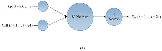
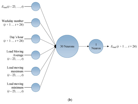
Figure 1.
Proposed artificial neural network (ANN) models. (a) feedforward ANN for photovoltaic (PV) generation and (b) feedforward ANN for load consumption forecasting.
Using the generation of the previous day as one of the two inputs allowed exogenous factors affecting production, which were not measured or quantified in this case, to be captured and considered by the ANN. Such parameters may reflect a partial loss of production due to module, string, and/or inverter failures, atmospheric pressure, PV panel soiling, and so on. On the other hand, as it is known that, (i) PV generation is highly correlated with sun’s radiation, (ii) irradiance forecasts from meteorological departments are commonly given for horizontal surfaces, and (iii) converting GHI to the actual irradiance hitting the PV modules (plane of array irradiance—PoA) is complex and not straightforward, GHI was chosen as the second input. With the aid of a trial and error approach, using root-mean-square error (RMSE) as the performance metric, 80 neurons in the hidden layer were used, with a sigmoid as their activation function, and 1 output neuron in the output layer with a linear activation function for giving the next day’s PV generation forecast. With this configuration, a RMSE (normalized) of 11% was obtained for the studied year.
Regarding the ANN used for the load consumption forecasting, Figure 1b, we followed a similar procedure to the PV forecast procedure explained above. The load consumption of the previous day was used in this case, as it was necessary to capture exogenous factors not measured or quantified in this case, such as ambient temperature, CO2 concentration, natural illuminance (ambient lighting), and so on. Moreover, the weekday number and the hour of the day for the forecasted period were used, as the load pattern was strongly correlated with the day of the week and the hour of the day. For instance, the load behaved differently in Sundays compared to Mondays and the peak load occurred—generally—in the afternoon. Finally, to improve the learning of the load profile, inputs such as the load’s moving average, the moving minimum, and moving maximum of the previous day were also used. With 30 neurons in the hidden layer with a sigmoid as their activation function and 1 neuron in the output layer possessing a linear activation function, a RMSE (normalized) of 6% was obtained for the studied year.
It is worth mentioning that in both networks, the training process was performed using the backpropagation learning algorithm and an annual training dataset obtained from a dwelling, located at Lat/Lon: 35.101765, 33.348838, for 2017. Finally, the ANN forecasts versus the measured values, by month against daily-hour average, are shown in Figure 2.
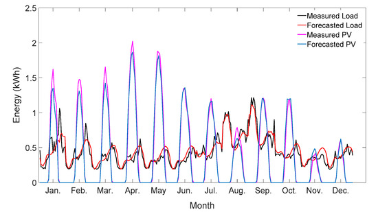
Figure 2.
Monthly daily-hour average of forecasted and measured PV and load.
To give a clearer understanding of the weather at the location under study, Figure 3 shows different weather-related parameters for one representative month per season in 2018. The representative months selected were January for winter, April for spring, July for summer, and October for autumn. By closely examining these parameters, one may conclude that in Cyprus the climate is significantly warm with high humidity levels. Despite the high temperature and humidity, which may affect the generation of PV systems, high irradiance levels are observed, leading to significant PV energy generation. On the other hand, the presence of high humidity and high temperatures leads to the intense use of cooling systems in summer, thus increasing the energy needs of buildings.
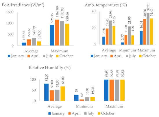
Figure 3.
Maximum, minimum, and average PV generation, PoA irradiance (including night-times), ambient temperature, and relative humidity at the location under study.
The data were monitored through a small weather station installed locally, using measuring equipment such as a pyranometer, temperature sensor, and humidity sensor. PV generation was measured automatically by the inverter installed at the inverter’s ac output, and load consumption was measured by a digital meter positioned at the beginning of the building’s installation. PV and weather data were available through the inverter’s integrated software, while load consumption data were available through a separate software package. PV and weather data were available in 15 min resolution, while load was available in hourly resolution.
2.4. Integrating ANN, GA, LP, and SAM
Integrating the three models introduced above allowed a battery dispatch to be globally optimized in real time, since historical, current, and future values for both PV and load were recurrently considered during the optimization horizon. Therefore, based on the input information mixture of the measured and forecasted values, the dispatch was repeated and rescheduled in an optimum manner for every time step (one hour) of the optimization horizon (24 h). As mentioned earlier, to address the non-linear and complex nature of the battery and model its performance in a more realistic manner, SAM was embedded in the proposed algorithm. The successful coupling of the proposed LP with SAM was previously reported in another study [30].
Specifically, at the end of each simulation day, the two ANNs forecast the next day’s PV generation and load consumption, while the GA, based on the forecasts, repeatedly ran the LP algorithm until the next day’s optimum weights were found. With the resulting optimum weights, a forecasted dispatch for the next 24 hours was attained through LP and the final dispatch was then obtained with the aid of SAM. In particular, once the LP dispatch was obtained from MATLAB, then the PV load and the desired battery optimum dispatch were imported into SAM. Here, the whole dispatch was recalculated by SAM, by following the given PV, load, and the desired LP dispatch obtained in MATLAB. If the desired LP dispatch required the battery to operate beyond its physical limits, then SAM recalculated the correct battery charge/discharge and the net grid energy, based on the energy balance equation and the available energy storage level of the battery at the current time step. During the real-time phase, at each time step, the matrices containing the PV and load forecasts were substituted by their corresponding measured values, the LP reran relying on the new, updated data, and SAM calculated the final dispatch based on the updated ideal battery dispatch from LP. Finally, at the end of the day, the resulting state of charge (SoC) of the battery calculated by SAM was used as the initial SoC of the next day. This procedure was repeated for each day of the simulation period, i.e., for one year in this case.
In Figure 4 and Figure 5, the aforementioned procedure is graphically demonstrated with the aid of a block diagram and a flowchart. It should be noted that in the algorithm’s flowchart shown in Figure 5, the parameters displayed on the right correspond to the output parameters of the current algorithm’s state, which are used as inputs by the algorithm’s next state. For instance, the state “GA weights optimization and LP”, in the block in which both the optimum weights and the forecasted dispatch are obtained, provides the next state’s inputs, such as the optimum ideal battery charging and discharging energies along with the day’s initial storage level.
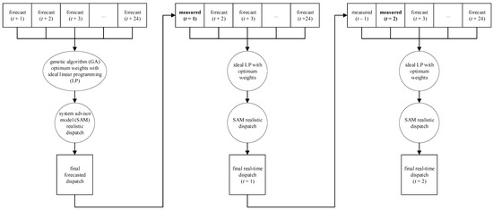
Figure 4.
Procedure for the forecasted and real-time optimum dispatches for a single day.
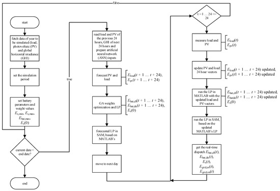
Figure 5.
Simulation algorithm flowchart.
Figure 6 shows an example of the proposed ANN-GA-LP-SAM model’s outcome, regarding the forecasted and real-time dispatches and the battery’s SoC, for a three day simulation period. A snapshot of the simulation, representing the forecasted dispatch for 24 January 2018 and the status of the real-time dispatch for the same day at 15:00, is shown in Figure 6a,b. The top diagrams show the expected dispatch and the battery’s SoC of the day, whereas the bottom diagrams show how both the dispatch and the battery’s SoC evolved in real-time when changes in PV and load occurred. Similarly, Figure 6c,d show the overall forecasted (or expected) dispatch and the battery’s SoC along with their evolution, in real-time, for the full three day simulation period. A visual comparison of the forecasted and measured values for both PV and load shows that a noticeable difference existed, resulting in a different from the expected dispatch. Despite the forecasting errors, due to the stochasticity of both the PV generation and load, it was clearly shown that the proposed model is able to adapt to such stochastic events and any uncertain changes, since the battery operated within its SoC limits and the energy balance was maintained at all times.
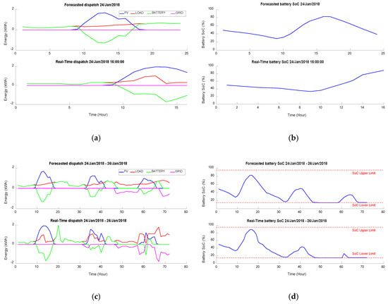
Figure 6.
Forecasted and real-time dispatch. (a) Forecasted dispatch for 24 January 2018 and real-time dispatch for 24 January 2018 (up to 15:00); (b) forecasted battery SoC for 24 January 2018 and real-time battery SoC for 24 January 2018 (up to 15:00); (c) forecasted vs. real-time dispatch for 24–26 January 2018 and (d) forecasted vs. real-time SoC for 24–26 January 2018. Storage capacity = 9.3 kWh.
3. Base Study Results
3.1. Simulation Data
According to the Cyprus Decree 121/2020, in summary, each new building (residential) shall be nZEB if it has a maximum primary energy consumption of 100 kWh/m2/year, utilizes thermal insulation, uses efficient energy systems for heating and cooling, and has integrated RES for covering its energy needs [41]. The building under study here had an integrated PV system of 3 kWp and was equipped with thermal double-glazed windows, 80 mm of thermal insulation across the building’s façade and roof, and dc inverter air-conditioning units for heating and cooling needs. As a base study, PV and load measurements for the period of 23 January 2018 to 22 January 2019 were taken from a residential building located in Nicosia, Cyprus.
With the PV and load data lying in the range of 15 min and hourly resolutions, respectively, the PV data were converted to an hourly resolution by simply aggregating the 15 min energy delivered in each hour. For instance, the hourly energy delivered at 08:00 am was the sum of the energy delivered at 07:15, 07:30, 07:45, and 08:00, and so on.
Figure 7, Figure 8 and Figure 9 represent the total PV energy generated and load consumption and their daily average profiles for the studied year. As can be observed, the highest PV energy levels were recorded in the 2nd quarter of the year (April–June), due to the high irradiance and relatively low temperatures, while the last quarter had the lowest production, due to the increased number of cloudy days. With an average of 12 hours daily generation (07:00–19:00), the concept of harvesting PV energy via storage in buildings constitutes a key part of the nZEB solution.
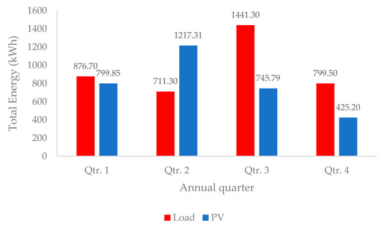
Figure 7.
Total PV generation and load consumption by quarter in 2018.
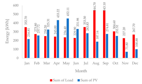
Figure 8.
Total PV generation and load consumption by month in 2018.
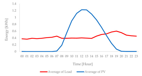
Figure 9.
Average 24 hour PV generation and load consumption for 2018.
Compared to PV generation, Figure 7, Figure 8 and Figure 9 show that the total building’s energy needs behaved in a relatively opposite manner. In particular, during quarters 2, 3, and 4, the load was either greater or lower than the PV, with the only exception occurring in quarter 1, where generation was close to consumption. Moreover, the annual peak consumption occurred in the 3rd quarter due to the increased cooling needs, the lowest consumption occurred in the 1st quarter due to the reduced cooling and heating needs, and, finally, the daily peak load occurred roughly at 20:00. With the high imbalance between generation and consumption (Figure 8), which is a common phenomenon with existing building PV installations, the handling of the daily and thus quarterly and annual mismatches is of great importance. As shown in the following sections, storage can enhance the daily self-consumption by significantly reducing both the grid import energy (primary energy needs) and the grid export energy, contributing toward nZEB attainment.
3.2. Proposed LP Model Cross-Validation with SAM
Due to the non-linear and complex behavior of batteries, SAM—a trusted software developed by NREL and used by academics and professionals—was employed in this study to give a realistic and final battery dispatch. The validity of SAM as well as its battery models and dispatch algorithms can be found in References [42,43,44,45,46,47].
Figure 10 shows the four different steps followed from the ideal battery dispatch toward the final and more realistic dispatch. According to our proposed mechanism, this was driven by LP and obtained by SAM. In particular, the battery dispatch was attained with the aid of the proposed model presented in Section 2.1 and Section 2.2. This way, the model was imported into SAM, where the battery internal losses, dc and ac power conversion efficiencies, and other complex calculations (e.g., SoC estimation, battery roundtrip efficiency, and so on) were applied.
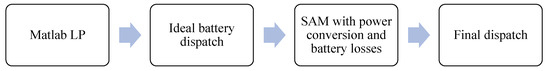
Figure 10.
From ideal battery dispatch to a more realistic dispatch.
As a case for the base study, the battery type used was a SAM model for a Li-ion nickel manganese cobalt oxide (NMC) battery with the main parameters mentioned in Table 1.

Table 1.
Battery Specifications.
To validate the proposed LP model, Figure 11 shows, for a ten day simulation period, the resulting hourly dispatch of the battery given by the LP model and the final dispatch given by SAM. As can be seen, due to the various non-linear and complex battery parameters, such as power losses and non-linear SoC estimation, the resulting final dispatch was slightly different from the one provided by LP. Specifically, the battery charging and discharging energies initially dispatched by the LP model were slightly lower and higher, respectively, due to the power losses of both the battery and the inverters.
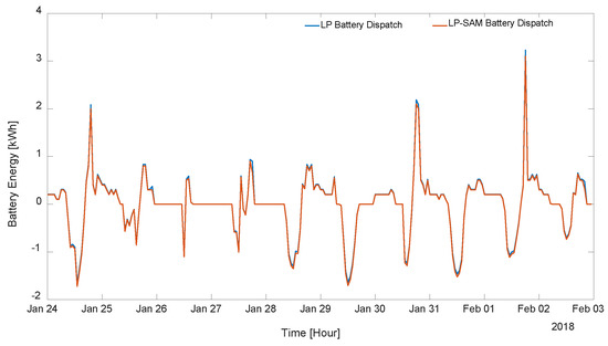
Figure 11.
Battery energy dispatch of LP and LP-SAM for a ten day simulation period with 9.3 kWh storage capacity. Positive energy means discharging and negative energy means charging.
The existence of such phenomena is also confirmed in Figure 12, where the annual daily average of the battery’s ideal profile was slightly higher than the more realistic dispatch. Nevertheless, it can clearly be observed that the profile of the LP model case was in a very good agreement with the case of SAM, which is globally accepted as realistic, indicating a very good precision for a valid model. The result of this comparison suggests that the combined LP-SAM model probably yielded an even more accurate model for implementation.
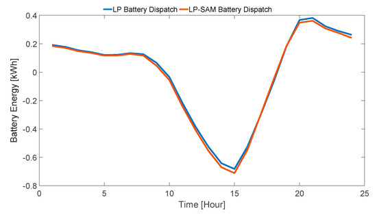
Figure 12.
Annual 24-hour average dispatch between the LP model and the combined LP-SAM model with a 9.3 kWh storage capacity.
3.3. Annual Net-Grid Energy and Self-Consumption
Maintaining low primary energy consumption needs in buildings and simultaneously maximizing the consumption from buildings’ RES (self-consumption) is vital and a key requirement for nZEBs. In this regard and from the electrical point of view, the concept of balancing (or equating) the annual load consumption with the annual PV generation by merely sizing the system, either with or without storage, does not necessarily achieve the best solution for maintaining the import energy at low levels and maximizing self-consumption, without making use of a global optimization dispatch scheme.
Even when the annual PV generation and load consumption are very close, a noticeable daily imbalance may exist, as shown in Figure 13, where the annual daily-hour average profiles of the net grid energy are presented for two different cases: (i) when no storage was used and (ii) when real-time global optimization dispatch, with storage, was utilized. When no storage was used, the REG was self-consumed only when there was PV generation, with the surplus energy exported to the grid, whereas in the second case, the nZEB requirement was further achieved, with the initial curve flattened and maintained closer to the reference line of 0 kWh.
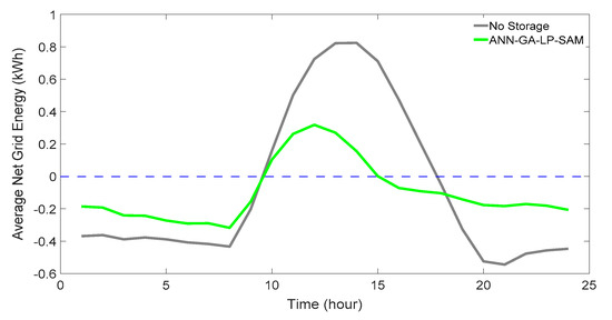
Figure 13.
Annual daily-hour average profile of net grid energy with 9.3 kWh storage capacity.
To further highlight the need for a real-time global optimization scheme, the proposed model was compared with a conventional default controller of SAM, known as a target controller [44]. By definition, this controller aims to maintain the grid energy at a level predefined by the user, and thus, it is possible to preserve the net-grid energy at low levels by simply defining a level of 0 kWh for each time step of the simulation period.
For comparison purposes, a parametric study was also conducted in order to observe the effect of three different storage sizes, 6 kWh, 9.3 kWh, and 11.4 kWh—chosen from residential batteries available in the market—leaving all parameters (see Table 1) other than the storage capacity unaltered. As a first outcome of the parametric study, Figure 14 illustrates the annual aggregated usage of the grid, described by the sum of the annual import and export energies. In this analysis, the three cases studied corresponded to scenarios where (i) no storage was used, (ii) when storage was used and dispatched by a conventional controller (target controller), and (iii) when storage was used and dispatched by the proposed global optimization scheme (ANN-GA-LP-SAM).
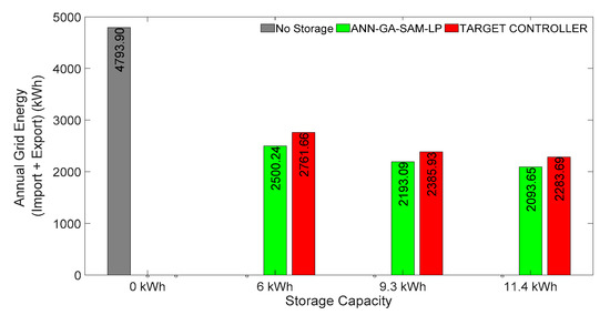
Figure 14.
Comparison of the annual total grid energy (import + export) for cases without storage, with target controller, and with the proposed model, for storage capacity cases of 6 kWh, 9.3 kWh and 11.4 kWh.
As can be observed, and as expected, the annual aggregated usage of the grid was much higher without storage, compared to the cases when storage was used. The case with the target controller returned an average (considering all battery sizes) reduction of ~48%. Finally, the case making use of the proposed global optimization scheme exhibited a further average reduction of 5% (total: ~53%), thus indicating the dominance of a real-time global optimization dispatch. Regardless of the further reduction in the aggregated usage of the grid as the battery sizes increased, as shown in Figure 14, it was found that with a battery size of 11.4 kWh, a minimum usage of ~2090 kWh was achieved. However, the use of larger batteries does not imply further improvement, due to the nature of the studied PV and load. Finally, the outcome presented in Figure 13 and Figure 14 is reflected in Figure 15, where the annual self-consumption seemed to be enhanced by application of the proposed model. Compared to the case without storage, self-consumption was almost double on average when storage was dispatched with the target controller, and a further average increase of 3% was achieved when storage was dispatched by our proposed paradigm.
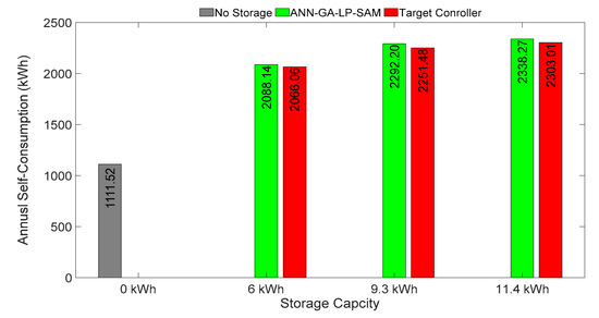
Figure 15.
Self-consumption for cases without storage, with target controller, and with the proposed model, for storage capacity cases of 6 kWh, 9.3 kWh, and 11.4 kWh.
As a final analysis, taking the high mismatch between the PV generation and load consumption into consideration (presented in Figure 7 and Figure 9, and further verified in Figure 13), the significant enhancement by the use of storage of self-consumption in each hour and season throughout the year are demonstrated, respectively, in Figure 16 and Figure 17. It is clearly shown here that without storage, there was a strong real-time mismatch between PV and load (Figure 16) and thus a low self-consumption.
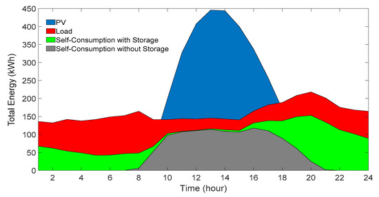
Figure 16.
Annual per daily-hour self-consumption without storage and with a 9.3 kWh storage, shown with PV generation and building load.
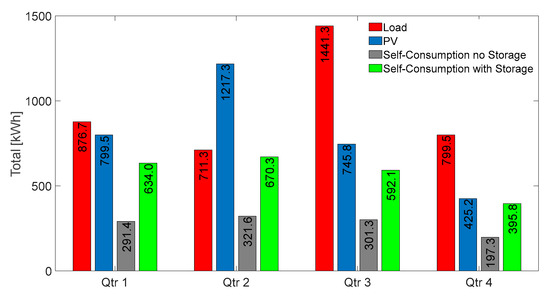
Figure 17.
Self-Consumption by quarter, for the year studied, without storage and with a storage of 9.3 kWh capacity, shown with PV generation and building load.
On the other hand, self-consumption was increased (Figure 17) when storage and real-time global optimization dispatch were considered, with the storage bringing self-consumption closer to either the load consumption or the PV generation in each of the annual quarters. Finally, the extended self-consumption throughout the day, due to the battery behavior driven by the proposed model, may be observed in Figure 16. It was clearly observed here that the battery stored the PV surplus energy and supplied the load when there was not enough PV generation. Owing to this dispatch scheme, and as one may conclude from Figure 17, 60% of the annual consumption was covered by the PV.
4. Conclusions and Discussion
This work aimed to meet the need for a new model able to minimize primary energy consumption from the electrical point of view, and to maximize a building’s renewable energy self-consumption through storage and a real-time optimization method within an nZEB. This was achieved through a novel and holistic integration of artificial intelligence (ANN) for PV and load forecasting, with a real-time hybrid optimization method (heuristic—GA, and convex—LP optimization), for battery energy management, and with a realistic battery dispatch software (SAM), for a more realistic battery dispatch. To the best of our knowledge, such an approach has never been attempted before to address the aforementioned aim. To this end, the current study showed the significant reduction of a building’s aggregated grid usage throughout the year in relation to the sum of import and export energies. Owing to this minimization, self-consumption was significantly enhanced, allowing a higher autonomy of the building.
It must be stressed that the current analysis mainly focused on zeroing the daily net electrical energy, as is expected for nZEBs. In the context of nZEB definitions, electricity prices, investment costs, operation and maintenance costs, and so on, do not necessarily act as a low energy target, and remained beyond the scope of this study. To use such factors/parameters in a problem such as the one presented here would limit its possible findings to the solutions to a specific and not a global problem, as these factors strongly rely on subsidies, loans, surplus energy sell price, electricity buying price, PV and battery prices, and so forth. Some of these (e.g., subsidies) may not even be available in many countries, and, more importantly, they may change in an unpredictable way, based on a country’s amendment of energy policies and/or energy economics. As a result, an optimized solution based on today’s situation may not be suitable for future times. On the other hand, addressing the sheer energy size and not its cost toward achieving low energy targets is a common and global problem that can be adopted irrespective of costs and prices.
Returning to this study’s findings, with the battery essentially acting as an “extension” of the PV generation throughout the day, a parametric study conducted using three different storage sizes showed that the average self-consumption could be increased by a factor of two, the annual aggregated grid usage (import + export energies) could be reduced by 53%, on average, and the annual load could be mostly supplied by the PV at a rate of 60%, as compared to the no-storage scenario. This shows the importance of having battery storage even in grid-connected PV systems. By accurately forecasting the PV generation and the load consumption (RMSE of 11% for PV and RMSE of 6% for load), verifying the accuracy of our model when it was cross-checked with a realistic software (SAM), and optimally driving the coupled LP-SAM model through GA, the adaptiveness of the model in real-time is observed, leading to better outcomes compared to a conventional, rule-based dispatch model. In this regard, researchers and professionals may be influenced toward the development of new controllers, in order to meet the desired energy levels of an nZEB in real-time. Based on our findings, the practical application of the proposed approach in each individual building can contribute toward an energy-efficient system. In particular, aiming the enhancement of an nZEB’s energy autonomy and its daily zeroing of the net grid energy, it is possible in a district to simultaneously achieve a higher penetration of distributed energy resources (DER) and a lower energy exchange between the buildings and the grids. This will also allow existing grids to adapt to these challenges, without the need for introduction of expensive and complicated mechanisms by the grid operators. However, this remains a challenge, as current policies within the EU need to alter to support and enable such schemes.
In every battery application, the battery’s aging (natural calendar aging and capacity fade due to the excess battery performance) constitutes an important factor when it comes to the concept of maximizing a battery’s life, and hence minimizing any potential economic damage. Nevertheless, the consideration of the associated battery degradation, the improvement of the forecasting model to further reduce the effect of errors due to the stochastic nature of the PV and load, and the result of a potential application in a cluster of buildings demand a further considerable effort and analysis, and constitute a naturally consequent study for the future.
Author Contributions
Conceptualization, G.S.G. and P.C.; methodology, G.S.G.; software, G.S.G. and P.N.; validation, P.C. and S.A.K.; formal analysis, G.S.G.; investigation, G.S.G.; resources, S.A.K.; data curation, G.S.G.; writing—original draft preparation, G.S.G. and P.N.; writing—review and editing, P.C. and S.A.K.; visualization, P.C. and G.S.G.; supervision, P.C. and S.A.K.; project administration, P.C. All authors have read and agreed to the published version of the manuscript.
Funding
This research received no external funding.
Acknowledgments
This work was supported by the Cyprus Department of Meteorology and Electricity Authority of Cyprus via their contribution to providing historical PV and weather forecasting data.
Conflicts of Interest
The authors declare no conflict of interest.
Abbreviations
| AI | artificial intelligence |
| ANN | artificial neural network |
| GA | genetic algorithms |
| GHI | global horizontal radiation |
| LP | linear programming |
| MPC | model predictive control |
| NREL | National Renewable Energy Laboratory |
| NWP | numerical weather prediction |
| nZEB | nearly-zero-energy building |
| PoA | plane of array |
| PV | photovoltaic |
| REG | renewable energy generation |
| RES | renewable energy sources |
| RMSE | root mean squared error |
| SAM | system advisor model |
| SoC | state of charge |
References
- Filippidou, F.; Jiménez Navarro, J.J. Achieving the Cost-Effective Energy Transformation of Europe’s Buildings; Publications Office of the European Union: Brussels, Belgium, 2019.
- U.S. Energy Information Administration. International Energy Outlook 2019; U.S. Energy Information Administration: Washington, DC, USA, 2019.
- U.S. Energy Information Administration. Building Sector Energy Consumption; U.S. Energy Information Administration: Washington, DC, USA, 2016.
- European Commission. Energy Performance of Buildings Directive. 2018. Available online: https://ec.europa.eu/energy/topics/energy-efficiency/energy-efficient-buildings/energy-performance-buildings-directive_en (accessed on 5 February 2020).
- European Parliment and The Council of the European Communities. Decision No 406/2009/EC of the European Parliament and of the Council of 23 April 2009 on the effort of Member States to reduce their greenhouse gas emissions to meet the Community’s greenhouse gas emission reduction commitments up to 2020. Off. J. Eur. Union 2009, L140, 136–148. [Google Scholar]
- Recast, E.P.B.D. Directive 2010/31/EU of the European Parliament and of the Council of 19 May 2010 on the energy performance of buildings (recast). Off. J. Eur. Union 2010, 18, 13–35. [Google Scholar]
- European Commission. Directive 2018/844/EU Energy performance of buildings. Off. J. Eur. Union 2018, 2018, 75–91. [Google Scholar]
- European Commission. Proposal for a Directive of the European Parliament and of the Council; European Commission: Brussels, Belgium, 2016. [Google Scholar]
- Sesana, M.M.; Salvalai, G. Overview on life cycle methodologies and economic feasibility fornZEBs. Build. Environ. 2013, 67, 211–216. [Google Scholar] [CrossRef]
- Sartori, I.; Napolitano, A.; Voss, K. Net zero energy buildings: A consistent definition framework. Energy Build. 2012, 48, 220–232. [Google Scholar] [CrossRef]
- Mangogna, A.; Valagussa, D.; Akintola, T.O.; Arietti, M.; Cicero, S.; Mordillo, F.; Pagani, A.; Sipione, R.; Corgnati, S.P. Towards nearly-zero energy buildings: HVAC system’s performances in the expected operative scenarios of Turin Energy Centre. In Proceedings of the REHVA Annual Conference “Advanced HVAC and Natural Gas Technologies”; Riga Technical University: Riga, Latvia, 2015; p. 8. [Google Scholar]
- Visa, I. Sustainable Energy in the Built Environment -Steps Towards nZEB—Proceedings of the Conference for Sustainable Energy (CSE) 2014; Springer: Cham, Switzerland, 2014. [Google Scholar]
- Baños, R.; Manzano-Agugliaro, F.; Montoya, F.; Gil, C.; Alcayde, A.; Gómez, J. Optimization methods applied to renewable and sustainable energy: A review. Renew. Sustain. Energy Rev. 2011, 15, 1753–1766. [Google Scholar] [CrossRef]
- Schimschar, S.; Surmeli, N.; Hermelink, A. Guidance Document for National Plans for Increasing the Number of Nearly Zero- Energy Buildings; ECOFYS: Cologne, Germany, 2013. [Google Scholar]
- Silva, P.C.; Almeida, M.; Braganca, L.; Mesquita, V. Development of prefabricated retrofit module towards nearly zero energy buildings. Energy Build. 2013, 56, 115–125. [Google Scholar] [CrossRef]
- Nottrott, A.; Kleissl, J.; Washom, B. Energy dispatch schedule optimization and cost benefit analysis for grid-connected, photovoltaic-battery storage systems. Renew. Energy 2013, 55, 230–240. [Google Scholar] [CrossRef]
- Hanna, R.; Kleissl, J.; Nottrott, A.; Ferry, M. Energy dispatch schedule optimization for demand charge reduction using a photovoltaic-battery storage system with solar forecasting. Sol. Energy 2014, 103, 269–287. [Google Scholar] [CrossRef]
- Chen, X.; Wei, T.; Hu, S. Uncertainty-Aware Household Appliance Scheduling Considering Dynamic Electricity Pricing in Smart Home. IEEE Trans. Smart Grid 2013, 4, 932–941. [Google Scholar] [CrossRef]
- Youn, L.T.; Cho, S. Optimal Operation of Energy Storage Using Linear Programming Technique. In Proceedings of the World Congress on Engineering and Computer Science, San Francisco, CA, USA, 20–22 October 2009. [Google Scholar]
- Rahmani-Andebili, M.; Shen, H. Energy Scheduling for a Smart Home Applying Stochastic Model Predictive Control. In Proceedings of the 2016 25th International Conference on Computer Communication and Networks (ICCCN); Institute of Electrical and Electronics Engineers (IEEE): Piscataway, NY, USA, 2016; pp. 1–6. [Google Scholar]
- Oh, E.; Son, S.-Y.; Hwang, H.; Park, J.-B.; Lee, K.Y. Impact of Demand and Price Uncertainties on Customer-side Energy Storage System Operation with Peak Load Limitation. Electr. Power Compon. Syst. 2015, 43, 1872–1881. [Google Scholar] [CrossRef]
- Wu, Z.; Tazvinga, H.; Xia, X. Demand side management of photovoltaic-battery hybrid system. Appl. Energy 2015, 148, 294–304. [Google Scholar] [CrossRef]
- Dargahi, A.; Ploix, S.; Soroudi, A.; Wurtz, F. Optimal household energy management using V2H flexibilities. COMPEL—Int. J. Comput. Math. Electr. Electron. Eng. 2014, 33, 777–792. [Google Scholar] [CrossRef]
- Wen, Y.-J.; Agogino, A.M. Wireless networked lighting systems for optimizing energy savings and user satisfaction. In Proceedings of the 2008 IEEE Wireless Hive Networks Conference; Institute of Electrical and Electronics Engineers (IEEE): Piscataway, NY, USA, 2008; pp. 1–6. [Google Scholar]
- Lauinger, D.; Caliandro, P.; Van Herle, J.; Kuhn, D. A linear programming approach to the optimization of residential energy systems. J. Energy Storage 2016, 7, 24–37. [Google Scholar] [CrossRef]
- Georgiou, G.S.; Nikolaidis, P.; Lazari, L.; Christodoulides, P. A Genetic Algorithm Driven Linear Programming for Battery Optimal Scheduling in nearly Zero Energy Buildings. In Proceedings of the 2019 54th International Universities Power Engineering Conference (UPEC), Piscataway, NY, USA, 3–6 September 2019; pp. 1–6. [Google Scholar]
- Lu, Y.; Wang, S.; Shan, K. Design optimization and optimal control of grid-connected and standalone nearly/net zero energy buildings. Appl. Energy 2015, 155, 463–477. [Google Scholar] [CrossRef]
- Ipsos Belgium and Navigant. Comprehensive Study of Building Energy Renovation Activities and the Uptake of Nearly Zero-Energy Buildings in the EU Final Report; European Commission: Brussels, Belgium, 2019. [Google Scholar]
- Cao, X.; Dai, X.; Liu, J. Building energy-consumption status worldwide and the state-of-the-art technologies for zero-energy buildings during the past decade. Energy Build. 2016, 128, 198–213. [Google Scholar] [CrossRef]
- Georgiou, G.S.; Christodoulides, P.; Kalogirou, S.A. Optimizing the energy storage schedule of a battery in a PV grid-connected nZEB using linear programming. Energy 2020. [Google Scholar] [CrossRef]
- The MathWorks, Inc. Solve Linear Programming Problems—MATLAB Linprog. Available online: https://www.mathworks.com/help/optim/ug/linprog.html (accessed on 10 June 2019).
- Boyd, S.; Vandenberghe, L. Convex Optimization; University of Cambridge: Cambridge, UK, 2010; Volume 25. [Google Scholar]
- Georgiou, G.S.; Christodoulides, P.; Kalogirou, S.A. Real-time Energy Convex Optimization, via electrical storage, in Buildings—A review. Renew. Energy 2019, 139, 1355–1365. [Google Scholar] [CrossRef]
- Mitchell, M. An Introduction to Generic Algorithms, 1st ed.; The MIT Press: London, UK, 1996. [Google Scholar]
- Garg, S.; Konugurthi, P.; Buyya, R. A linear programming-driven genetic algorithm for meta-scheduling on utility grids. Int. J. Parallel. Emergent Distrib. Syst. 2011, 26, 493–517. [Google Scholar] [CrossRef]
- Konugurthi, P.K.; Ramakrishnan, K.; Buyya, R. A Heuristic Genetic Algorithm based Scheduler for “Clearing House Grid Broker”; Grid Computing and Distributed Systems Laboratory: Parkville, Australia, 2007; pp. 1–9. Available online: http://cloudbus.cis.unimelb.edu.au/reports/ClearingHoseBroker2007.pdf (accessed on 5 February 2020).
- Nikolaidis, P.; Poullikkas, A. Enhanced Lagrange relaxation for the optimal unit commitment of identical generating units. IET Gener. Transm. Distrib. 2020, 1, 2–13. [Google Scholar] [CrossRef]
- Samarasinghe, S. Neural Networks for Applied Sciences and Engineering: From Fundamentals to Complex Pattern Recognition, 1st ed.; Taylor and Francis Group: New York, NY, USA, 2007. [Google Scholar]
- Jain, A.K.; Mao, J.; Mohiuddin, K.M. Artificial neural networks: A tutorial. Computer (Long. Beach. Calif) 1996, 29, 31–44. [Google Scholar] [CrossRef]
- Mellit, A.; Kalogirou, S. Artificial intelligence techniques for photovoltaic applications: A review. Prog. Energy Combust. Sci. 2008, 34, 574–632. [Google Scholar] [CrossRef]
- Republic of Cyprus: Ministry of Energy, Commerce Industry & Tourism. Cyprus Decree KDP 121/2020: Building Energy Performance Regulation; Governemtn Printing Office: Nicosia, Cyprus, 2020.
- Rudié, E.; Thornton, A.; Rajendra, N.; Kerrigan, S. System Advisor Model Performance Modeling Validation Report: Analysis of 100 Sites; Locus Energy LLC: Hoboken, NJ, USA, 2014. [Google Scholar]
- Freeman, J.; Whitmore, J.; Kaffine, L.; Blair, N.; Dobos, A.P. System Advisor Model: Flat Plate Photovoltaic Performance Modeling Validation Report. In System Advisor Model: Flat Plate Photovoltaic Performance Modeling Validation Report; National Renewable Energy Laboratory: Golden, CO, USA, 2013. [Google Scholar]
- Diorio, N. An Overview of the Automated Dispatch Controller Algorithms in the System Advisor Model (SAM); National Renewable Energy Laboratory: Golden, CO, USA, 2017.
- Diorio, N.; Dobos, A.; Janzou, S.; Nelson, A.; Lundstrom, B. Technoeconomic Modeling of Battery Energy Storage in SAM; National Renewable Energy Laboratory: Golden, CO, USA, 2015.
- Freeman, J.; Whitmore, J.; Blair, N.; Dobos, A.P. Validation of Multiple Tools for Flat Plate Photovoltaic Modeling Against Measured Data; National Renewable Energy Laboratory: Golden, CO, USA, 2014.
- Blair, N.; Dobos, A.; Sather, N. Case studies comparing system advisor model (SAM) results to real performance data. In Proceedings of the World Renewable Energy Forum, WREF 2012, Including World Renewable Energy Congress XII and Colorado Renewable Energy Society (CRES) Annual Conference, Denver, CO, USA, 13–17 May 2012; Volume 4, pp. 2698–2703. [Google Scholar]


© 2020 by the authors. Licensee MDPI, Basel, Switzerland. This article is an open access article distributed under the terms and conditions of the Creative Commons Attribution (CC BY) license (http://creativecommons.org/licenses/by/4.0/).