Fractional-Order Finite-Time, Fault-Tolerant Control of Nonlinear Hydraulic-Turbine-Governing Systems with an Actuator Fault

Abstract

Hydropower units undertake tasks such as peak shaving, frequency modulation, and providing accident reserves in the power system. With the increasing capacity and structural complexity of power systems, hydropower units have become more important. Hydraulic-turbine-governing systems (HTGSs) need to have higher control performance and automation levels to meet the higher regulatory requirements of the power system. To achieve high-quality control, we proposed a new finite-time, fault-tolerant control method for HTGSs with an actuator fault. First, a fractional-order model for HTGSs with uncertainty, external disturbance, and an actuator fault was introduced. Second, a fault estimator that could quickly track the fault signal for an actuator fault was proposed. Then, based on the fractional-order finite-time stability theorem, a finite-time, fault-tolerant controller was proposed for the stabilization of an HTGS. Furthermore, a controller was developed as a fractional differential form combined with a smooth bounded arctangent function to effectively suppress jitters and uncertainties. Finally, numerical experimental results verified the validity and robustness of the proposed scheme.

1. Introduction

As the most important clean energy source, hydropower has made a major contribution to building clean, low-carbon, safe, and energy-efficient systems [1,2,3,4]. The world’s first million-kilowatt turbine for the hydropower "Big Mac" Baihetan Power Station has been completed. The use of supergiant hydroelectric generator units is continually increasing [5], and this will foster the need for higher requirements for the safe and stable operation of hydropower station systems [6,7,8]. A hydraulic-turbine-governing system (HTGS) is an important part of a hydropower station system and affects the safe and stable operation of the entire set of hydroelectric generator units and even the grid system [9,10,11]. At present, many hydropower-generating units at large- and medium-sized hydropower stations suffer from different degrees of stability problems [12,13,14]. Therefore, the stability and effective control of an HTGS is vital.

Fractional calculus is a generalization of differentiation and integration to an arbitrary order [15]. It has significant advantages in describing practical systems with memory, strong dependence, viscoelasticity, and genetic properties [16,17]. Many fractional models that are more in line with engineering practice have been established, e.g., in electromechanics [18], thermal systems [19], electrical engineering [20], etc. An HTGS is a complex nonlinear system integrating hydraulic, mechanical, and electrical components. For a long time, linear and integer-order modeling were mainly used [21,22,23,24]. Given the advantages of fractional calculus over integer calculus in describing complex and historically dependent systems, some work has been done in introducing fractional calculus to establish mathematical models of HTGSs [25]. Given the strong historical dependence of the hydraulic servo component, a fractional-order model that can better reflect the actual operating conditions was considered in this study.

Proportional-integral-derivative (PID) control is a classical and widely used scheme for HTGSs. Dounis et al. [22] studied a fuzzy PID controller by using a genetic algorithm to effectively improve the control quality of a hydraulic-turbine-regulating system with an elastic water hammer effect. Ge et al. [23] proposed a deterministic chaotic mutation evolutionary programming method for the online PID parameter optimization of hydro-turbine-regulating systems. Although the conventional PID control algorithm has the characteristics of a small number of calculations, easy implementation, and good real-time performance, the regulation time is long, and the oscillations are serious, which is adverse to the stable operation of the unit. Moreover, the PID parameters are set only for several working conditions. The adaptability is weak, especially in light of today’s increasing high demand for flexible operation. With the continuous improvement of control strategies, some novel control algorithms, such as adaptive control, fuzzy control, and neural network control, have emerged [24,25,26]. These algorithms have important practical and theoretical value for controlling HTGSs but they all have certain defects. For example, the adaptive control time is relatively long and cannot meet the characteristics of real-time control. The fuzzy control and neural network control algorithms have lower precision and slower response speed.

Most of the above control schemes have been proposed based on the assumption that actuators, sensors, and internal components do not fail. In fact, these parts are very prone to failure. In particular, actuators are more prone to various faults because of the presence of moving parts [27,28,29]. The electro-hydraulic servo system converts and amplifies the electrical signals sent by the electronic regulator into corresponding mechanical signals, and then it operates the vanes. It acts as an actuator in the regulation system. The main pressure-regulating valve is shown in Figure 1a,b. The main pressure-regulating valve converts the received electrical control signal into a hydraulic signal output and operates the relay after power amplification. The relay pushes the water guide vane of the hydro-turbine to adjust the water flow, thereby enabling control of the rotational speed of the hydroelectric generator set. A failure of the main pressure-regulating valve can have a serious impact on the entire actuator. For example, if the valve sleeve is seriously worn or the piston contacts a foreign object, the main pressure-regulating valve will be stuck, which will affect the normal operation of the servo; if the main pressure regulating valve is affected by oil staining or the oil temperature, the zero drift of the electro-hydraulic servo system will be too large; if an oil pressure imbalance occurs in the main pressure regulating valve, it will affect the stable operation of the relay. In addition, other faults may occur in the electro-hydraulic servo system; these include jamming of the pilot valve and swinging or crawling of the servomotor.

Fault-tolerant control can eliminate or resist the impact of the fault such that the system can maintain good performance and still achieve the expected control target [30,31,32]. As a self-contained structure, the HTGS requires long-time, high-power, and high-load continuous operation of automatic equipment. It is especially important to ensure that the safe operation of the system can be guaranteed and better performance can be maintained, even in the event of a component or subsystem failure. There are few reports on the fault-tolerant control of HTGSs. In addition, if the transient transition process of the HTGS is too long, it may cause greater damage to the hydropower system. Finite-time control can ensure that the system stabilizes in a fixed time and has the advantage of improving the system transition process [33,34,35]. Both fault-tolerant control for resisting faults or failures and finite-time control for improving the transition process have potential advantages, making them highly beneficial for high-quality control of hydropower systems. Therefore, can fault-tolerant control be combined with finite-time theory for the stability of fractional-order HTGSs? If the hypothesis is valid, what are the synthesized controller form and the specific mathematical derivation? This has not been addressed yet. The solution to this problem is important for improving the fault tolerance and high-quality control of HTGSs.

Based on the above analysis, the main contributions of our study are as follows. Given the strong historical dependence of the hydraulic servo component, a fractional-order nonlinear HTGS model with uncertainty, an external disturbance, and an actuator fault was presented. To quickly track the change of the fault signal when an actuator fault occurs, a finite-time fault estimator was proposed. Then, based on the fault estimator and the fractional-order finite-time stability theorem, a suitable sliding surface and a finite-time, fault-tolerant controller were designed for the fractional-order HTGSs such that the system state can converge to the sliding mode and reach a stable state in a finite time in the event of an actuator fault. In addition, the controller was developed in a fractional differential form combined with a smooth bounded arctangent function to effectively suppress jitters and uncertainties, demonstrating its good robustness. Finally, numerical experimental results verified the effectiveness of the proposed finite-time, fault-tolerant control scheme. There are many different types of faults in the hydraulic servo system of the HTGS, which will affect the normal operation of the hydraulic unit and even the hydropower station. This method can effectively resist the fault of the hydraulic servo system due to ensuring the stable operation of the HTGS and also provides a reference for fault-tolerant control of other hydropower systems.

2. Preliminaries and System Description

2.1. Definition of Fractional Calculus

There are three definitions of fractional calculus, namely, the Grünwald–Lrtnikov (G-L), Riemann–Liouville (R-L), and Caputo definitions. The scientific rationale of these definitions of fractional calculus has been verified in practice. Next, the definition of R-L fractional calculus and some properties used in this paper are introduced.

Definition 1. 

[36]: The fractional-order R-L derivative of functions $f\left(t\right)$ is defined as follows:

$${}_{t_0}{D}_t^{\alpha }f(t)=\frac{1}{\Gamma (m-\alpha )}\frac{d^m}{d{t}^m}{\displaystyle {\int }_{t_0}^t\frac{f(\tau )}{{(t-\tau )}^{\alpha -m+1}}}d\tau$$

(1)

for any real number $m-1<\alpha <m$, $m\in N$, where $t_0$and $t$ are the limits of operation of ${}_{t_0}{D}_t^{\alpha }f(t)$and $\Gamma (\cdot )$is the gamma function.

The R-L integral of fractional order is defined as:

$${}_{t_0}{I}_t^{\alpha }f(t)=D_t^{-\alpha }f(t)=\frac{1}{\Gamma (-\alpha )}{\displaystyle {\int }_{t_0}^t\frac{f(\tau )}{{(t-\tau )}^{\alpha +1}}}d\tau$$

(2)

for $\alpha$, $t_0\in R$, $\alpha <0$.

Property 1. 

[36]: For the R-L fractional derivative, the following holds:

$${}_{t_0}^{RL}{D}_t^{-\alpha }({}_{t_0}^{RL}{D}_t^{\beta }f(t))={}_{t_0}^{RL}{D}_t^{\beta -\alpha }f(t)-{\displaystyle \sum _{j=1}^m{\left[{}_{t_0}^{RL}{D}_t^{\beta -j}f(t)\right]}_{t=t_0}\frac{{(t-t_0)}^{\alpha -j}}{\Gamma (1+\alpha -j)}}, (0\le m-1\le \beta \le m).$$

(3)

Later in this paper, the $\alpha$-order R-L fractional derivative will be represented by the symbol $D^{\alpha }$.

2.2. Fractional-Order Finite-Time Stability

Lemma 1. 

[37]: Let $x=0$ be the stability point of the following fractional-order nonlinear system:

$$D^{\alpha }x(t)=f(x,t).$$

(4)

Suppose there is a Lyapunov function $V(t,x(t))$ and a class-$K$ function that satisfies:

$${\alpha }_1(‖x‖)<V(t,x(t))<{\alpha }_2(‖x‖), D^{\alpha }V(t,x)\le -{\alpha }_3(‖x‖),$$

(5)

where$\alpha \in (0,1)$; then, the system in Equation (4) will stabilize at the equilibrium point in a finite time.

Lemma 2. 

For any given real number x, the following inequality can be obtained:

$$x\arctan (x)=\left|x\arctan (x)\right|=\left|x\right|\left|\arctan (x)\right|\ge 0.$$

(6)

Proof. 

Letting $f(x)=x\arctan (x)$, for all real numbers x, one obtains:

$$f(-x)=(-x)\arctan (-x)=(-x)\left[-\arctan (x)\right] =x\arctan (x)=f(x).$$

(7)

Therefore, $f(x)$ is an even function. One thus obtains: $f(x)=f(-x)=\left|f(x)\right|=\left|x\arctan (x)\right| =\left|x\right|\left|\arctan (x)\right|\ge 0$ This completes the proof. □

Lemma 3. 

[38]: If $R(\alpha )>0$, the fractional integrals $I_{a+}^{\alpha }$ and $I_{b-}^{\alpha }$ are bounded; that is:

$$(1) {‖I_{a+}^{\alpha }x‖}_{L_P(a,b)}\le K{‖x‖}_{L_P(a,b)}, {‖I_{b-}^{\alpha }x‖}_{L_P(a,b)} \le K{‖x‖}_{L_P(a,b)}\left[K=\frac{{(b-a)}^{R(\alpha )}}{R(\alpha )\left|\Gamma (\alpha )\right|}\right].$$

(8)

(2) If $0<\alpha <1$ and $1<p<1/\alpha$, then $I_{a+}^{\alpha }$ and $I_{b-}^{\alpha }$ are bounded between $L_P(a,b)$ and $L_q(a,b)$, where $q=p/(1-\alpha p)$.

Remark 1.

Lemma 3(1) has been proved in Samko. and Vakulov. [39]. Lemma 3(2) is known as the Hardy–Littlewood theorem in Samko et al. [40].

2.3. Non-Linear Model of an HTGS

An HTGS is composed of a hydraulic turbine, a generator, a hydraulic servo system, and a load, which can be described as Ling. [41]:

$$\left\{\begin{array}{l}\dot{\delta }={\omega }_0\omega \\ \dot{\omega }=\frac{1}{T_{ab}}\left[m_t-D\omega -\frac{E_q^{\prime }{V}_s}{x_{d\sum }^{\prime }}\sin \delta -\frac{V_s^2}{2}\frac{x_{d\sum }^{\prime }-x_{q\sum }}{x_{d\sum }^{\prime }{x}_{q\sum }}\sin 2\delta \right]\\ {\dot{m}}_t=\frac{1}{e_{qh}{T}_w}\left[-m_t+e_{y}y+\frac{e{e}_y{T}_w}{T_y}y\right]\\ \dot{y}=-\frac{1}{T_y}y\end{array}\right. ,$$

(9)

where $\delta$ is the generator rotor angle; $\omega$ is the generator speed relative deviation; ${\omega }_0=2\pi f_0$; $m_t$ and $y$ are the relative values of torque $M_t$ and vane opening $Y$, respectively; $T_{ab}$ is the unit and load inertia time constant; $D$ is the generator damping coefficient and is generally regarded as a constant; $E_q^{\prime }$ is the q-axis transient potential; $V_s$ is the infinite bus voltage; $x_d^{\prime }$ and $x_q$ are generator d-axis transient reactance and q-axis synchronous reactance, respectively; $e_{qh}$ is the hydro-turbine flow to the head transfer coefficient; $T_w$ is the water flow inertia time constant of the pressure water diversion system; $e_y$ is the hydro-turbine torque to the vane opening; $e$ is the hydro-generator unit self-adjusting coefficient; and $T_y$ is the relay reaction time constant.

In actual operation, owing to uncertainties, such as the complexity of the HTGS, the interference of external noise, and the limitation of the observation capability, it is difficult to quantify the parameters of the system. In addition, the HTGS may also be subject to changes in the external environment, such as random interference caused by load disturbances. To better describe the actual operating conditions of the HTGSs, an uncertainty and a disturbance are added to the HTGS (Equation (9)).

The HTGS mainly controls the change of the flow rate by controlling the degree of vane opening to affect the rotational speed of the hydro-turbine unit. Therefore, during the operation of the hydro-turbine, the actuator that controls the opening of the vane is critical to the safety and reliability of the system. An actuator fault may cause unimaginable consequences; therefore, an actuator fault is considered in the HTGS (Equation (9)).

If $u_{pi}$ is used to design the controller and $u_i$ is the controller after the fault, then, when an actuator fault occurs:

$$u_i={\epsilon }_i(t)u_{pi}+{\phi }_i(t),$$

(10)

where ${\epsilon }_i(t)\in (0,1]$ is a continuous time-varying function that indicates the degree of the fault of the actuator. When ${\epsilon }_i(t)=1$, the actuator does not fail. The smaller ${\epsilon }_i(t)$ is, the greater the degree of the actuator fault; ${\phi }_i(t)$ denotes the deviation of the actuator.

In summary, by considering the fractional dynamics of the hydraulic servo component, an HTGS with uncertainties, external disturbances, and actuator faults can be presented as:

$$\left\{\begin{array}{l}\dot{\delta }={\omega }_0\omega +\Delta f_1(\delta ,t)+d_1^f(t)+u_1\\ \dot{\omega }=\frac{1}{T_{ab}}\left[m_t-D\omega -\frac{E_q^{\prime }{V}_s}{x_{d\sum }^{\prime }}\sin \delta -\frac{V_s^2}{2}\frac{x_{d\sum }^{\prime }-x_{q\sum }}{x_{d\sum }^{\prime }{x}_{q\sum }}\sin 2\delta \right],\\ +\Delta f_2(\omega ,t)+d_2^f(t)+u_2\\ {\dot{m}}_t=\frac{1}{e_{qh}{T}_w}\left[-m_t+e_{y}y+\frac{e{e}_y{T}_w}{T_y}y\right]+\Delta f_3(m_t,t)+d_3^f(t)+u_3\\ D^{\alpha }y=-\frac{1}{T_y}y+\Delta f_4(y,t)+d_4^f(t)+{\epsilon }_4(t)u_{p4}+{\phi }_4(t)\end{array}\right.$$

(11)

where $\alpha \in \left(0,1\right)$ is the fractional order of the system, and $\Delta f_i\left(x,t\right)\in R$ and $d_i^f\left(t\right)\in R$,$i=1,2,3,4$, denote the system’s uncertainties and external disturbances, respectively.

3. Finite-Time, Fault-Tolerant Controller Design

3.1. Fault Estimator Design

The fault-tolerant control method adopted in this paper is an active fault-tolerant control method, which is different from fault isolation and the diagnosis of traditional fault-tolerant control. In this section, we present the design for a fault estimator that can effectively track changes in fault signals after a fault has occurred and can be directly applied to the controller to compensate for the effects of the fault. First, a method for the equivalent separation of the controller after the failure was proposed. The controller was divided into a normal part and a fault-affected part, and the fault estimator was designed for the latter. Then, the finite-time stability of the fault estimator was given.

To effectively compensate for the impact of the system fault, the controller in Equation (10) that characterizes the actuator fault is first separated. By further treatment of Equation (10), the controller can be rewritten as:

$$u_i=u_{pi}-\left[(1-{\epsilon }_i(t))u_{pi}-{\phi }_i(t)\right].$$

(12)

Letting $u_{fi}=\left(1-{\epsilon }_i\left(t\right)\right)u_{pi}-{\phi }_i\left(t\right)$, we can represent Equation (12) as:

$$u_i=u_{pi}-u_{fi},$$

(13)

where $u_{pi}$ is the normal control part and $u_{fi}$ is the fault affected part. The fault estimator designed below is for $u_{fi}$.

Define $z=D^{\alpha -1}{X}_i$ such that $\dot{z}=D^{\alpha }{X}_i$. We can write Equation (11) as:

$$\dot{z}=D^{\alpha }{X}_i=f(x,t)+\Delta f(x,t)+d^f(t)+u_p-u_f.$$

(14)

Let vector $\sigma (t)$ be the solution of the following recursive equation:

$$\sigma (t)=\vartheta {\displaystyle {\int }_0^t\left(f(x,t)+\Delta f(x,t)+d^f(t)+u_p-\sigma (\phi )\right)}d\phi -\vartheta z,$$

(15)

where $\vartheta$ is a positive definite symmetric matrix.

Taking the first derivative with respect to time of Equation (15) gives:

$$\dot{\sigma }(t)=-\vartheta \sigma (t)+\vartheta u_f,$$

(16)

Because $\sigma \left(t\right)$ is obtainable exactly, to get the unknown actuator fault vector $u_f$, the estimate of $\sigma \left(t\right)$ can be described as:

$$\dot{\widehat{\sigma }}(t)=-\vartheta \widehat{\sigma }(t)+\vartheta {\widehat{u}}_f,$$

(17)

where $\widehat{\sigma }(t)$ and ${\widehat{u}}_f$ are the estimates of $\sigma (t)$ and $u_f$, respectively.

Define a sliding variable $\theta$ as:

$$\theta ={\vartheta }^{-1}(\sigma (t)-\widehat{\sigma }(t)).$$

(18)

The proposed fault estimator is:

$${\widehat{u}}_f=k_1\frac{\theta }{{‖\theta ‖}^{\frac{1}{2}}}-\vartheta \theta -w,$$

(19)

$$\dot{w}=-k_{2}sign(\theta ),$$

(20)

where $k_1$ and $k_2$ are positive scalars and $sign\left(\cdot \right)$ is the sign function.

Taking the first derivative with respect to time of Equation (18) gives:

$$\dot{\theta }=-\vartheta \theta +u_f-{\widehat{u}}_f.$$

(21)

By substituting Equation (19) into Equation (21), one obtains:

$$\dot{\theta }=-k_1\frac{\theta }{{‖\theta ‖}^{\frac{1}{2}}}+w+u_f.$$

(22)

If we define $\partial =w+u_f$, then Equations (20) and (22) can be represented as:

$$\dot{\theta }=-k_1\frac{\theta }{{‖\theta ‖}^{\frac{1}{2}}}+\partial ,$$

(23)

$$\dot{\partial }=-k_{2}sign(\theta )+{\dot{u}}_f.$$

(24)

Assumption 1. 

The actual output is bounded because of physical limitations during the actual operation of the actuator. The rate of change of the actuator fault can be considered bounded with a range of $‖u_f‖\le \epsilon$, which is a known positive scalar.

Theorem 1. 

For a linear system described by Equation (16), by applying the sliding dynamics in Equations (23) and (24) and Assumption 1, sliding motion can be achieved in a finite time and the amplitude of the actuator faults can be exactly estimated.

Proof. 

A candidate Lyapunov function in the following form is employed:

$$V={\chi }^{T}P\chi ,$$

(25)

where $\chi ={\left[\frac{{\theta }^T}{{‖\theta ‖}^{\frac{1}{2}}},{\partial }^T\right]}^T$ and $P=\frac{1}{2}\left(\begin{array}{cc}{k}_1^2+4k_2& -k_1\\ -k_1& 2\end{array}\right)$.

The first derivative of $V$ with respect to time can be obtained as:

$$\dot{V}=\left(\frac{k_1^2}{2}+2k_2\right)\frac{{\theta }^T\dot{\theta }}{‖\theta ‖}+2{\partial }^T\dot{\partial }-k_1\left(-\frac{1}{2}\frac{({\theta }^T\dot{\theta })({\partial }^T\theta )}{{‖\theta ‖}^{\frac{5}{2}}}+\frac{({\dot{\partial }}^T\theta +{\partial }^T\dot{\theta })}{{‖\theta ‖}^{\frac{1}{2}}}\right).$$

(26)

Substituting $\dot{\theta }$ and $\dot{\partial }$ from Equations (23) and (24) into Equation (25), one obtains:

$$\begin{array}{c}\dot{V}=-\left(\frac{k_1^3}{2}+k_1{k}_2\right)\frac{{‖\theta ‖}^2}{{‖\theta ‖}^{\frac{3}{2}}}+k_1^2\frac{{\theta }^T\partial }{‖\theta ‖}+\frac{k_1}{2}\frac{({\theta }^T\partial )({\partial }^T\theta )}{{‖\theta ‖}^{\frac{5}{2}}} -k_1\frac{({\partial }^T\partial )}{{‖\theta ‖}^{\frac{1}{2}}}+2{\partial }^T{\dot{u}}_f-k_1\frac{{\dot{u}}_f^T\theta }{{‖\theta ‖}^{\frac{1}{2}}}\\ \le -\left(\frac{k_1^3}{2}+k_1{k}_2\right){‖\theta ‖}^{\frac{1}{2}}+k_1^2\frac{‖{\theta }^T\partial ‖}{‖\theta ‖}+\frac{k_1}{2}\frac{{‖{\theta }^T\partial ‖}^2}{{‖\theta ‖}^{\frac{5}{2}}} -k_1\frac{‖{\partial }^T\partial ‖}{{‖\theta ‖}^{\frac{1}{2}}}+2‖{\partial }^T{\dot{u}}_f‖+k_1\frac{‖{\dot{u}}_{{}_f}^T\theta ‖}{{\theta }^{\frac{1}{2}}}\\ \le -\left(\frac{k_1^3}{2}+k_1{k}_2\right){‖\theta ‖}^{\frac{1}{2}}+k_1^2‖\theta ‖-\frac{k_1}{2}\frac{{‖\partial ‖}^2}{{\theta }^{\frac{1}{2}}}+2\epsilon ‖\partial ‖+k_1\epsilon {‖\theta ‖}^{\frac{1}{2}}\\ \rho ={\left[{‖\theta ‖}^{\frac{1}{2}},{\partial }^T\right]}^T,\end{array}$$

(27)

where $\rho ={\left[{‖\theta ‖}^{\frac{1}{2}},{\partial }^T\right]}^T$ and $Q=\frac{1}{2}\left(\begin{array}{cc}{k}_1^3+2k_1{k}_2-2\epsilon k_1& -(k_1^2+2\epsilon )\\ -(k_1^2+2\epsilon )& k_1\end{array}\right)$.

If $k_1>\sqrt{2\epsilon }$ and $k_2>3\epsilon +2{\epsilon }^2/k_1^2$, then $Q$ is a positive definite symmetric matrix. From Equation (27), we obtain:

$$\dot{V}\le -\frac{1}{{‖\theta ‖}^{\frac{1}{2}}}\lambda \min (Q){‖\rho ‖}^2,$$

(28)

where $\lambda \min (Q)$ is the minimum eigenvalue of $Q$.

Since $‖\rho ‖=‖\chi ‖$, then:

$$\dot{V}\le -\frac{1}{{‖\theta ‖}^{\frac{1}{2}}}\lambda \min (Q){‖\chi ‖}^2.$$

(29)

Similarly, the Lyapunov function in Equation (25) can be written as:

$$V\le \lambda \max (P){‖\chi ‖}^2,$$

(30)

where $\lambda \max (P)$ is the maximum eigenvalue of $P$.

Therefore:

$$\dot{V}\le -\frac{1}{{‖\theta ‖}^{\frac{1}{2}}}\frac{\lambda \min (Q)}{\lambda \max (P)}V.$$

(31)

Because $V^{\frac{1}{2}}>\sqrt{\lambda \min (P)}{‖\theta ‖}^{\frac{1}{2}}$, it follows that:

$$\dot{V}\le -\gamma V^{\frac{1}{2}},$$

(32)

where $\gamma =\frac{\lambda \min (Q)\sqrt{\lambda \min (P)}}{\lambda \max (P)}$.

According to the convergence result, there exists a finite time:

$$T_r=2V{(0)}^{\frac{1}{2}}/\gamma ,$$

(33)

where $V(0)$ is the initial value of $V$. Therefore, for all $t\ge T_r$, $\theta =\dot{\theta }=0$.

From Equation (19), we can obtain that, when $D^{\alpha }{x}_i(t)=f_i(x,t)+\Delta f_i(x,t)+d_i(t)+u_{pi}-u_{fi}$, the unknown actuator fault can be accurately estimated in a finite time:

$${\widehat{u}}_f=-w,$$

(34)

and it can be seen from Equation (21) that when $t\ge T_r$:

$${\widehat{u}}_f=u_f.$$

(35)

Thereby, the proof is completed. □

3.2. Controller Design

In this section, a finite-time, fault-tolerant control scheme based on the fractional-order finite-time stability theorem for HTGSs with uncertainty, an external disturbance, and an actuator fault is designed.

For convenience the HTGS in Equation (11) is rewritten as:

$$D^{\alpha }{x}_i(t)=f_i(x,t)+\Delta f_i(x,t)+d_i(t)+u_{pi}-u_{fi},$$

(36)

where $\alpha \in (0,1)$ is the fractional order of the system, $x(t)={\left[x_1,x_2,x_3,x_4\right]}^T\in R^n$ are system state variables, $f_i(x,t)={\left[f(x_1,t),f(x_2,t),f(x_3,t),f(x_4,t)\right]}^T\in R^n$ are the nonlinear functions of the system, and $\Delta f_i(x,t)={\left[\Delta f(x_1,t),\Delta f(x_2,t),\Delta f(x_3,t),\Delta f(x_4,t)\right]}^T\in R^n$ and $d_i(t)={\left[d_1(t),d_2(t),d_3(t),d_4(t)\right]}^T\in R^n$ are the uncertain and external disturbance terms of the system, respectively.

Assumption 2. 

In practice, the uncertainty of the system is unknown but the range can be estimated. The disturbances of the system are small and these disturbances are generally bounded. Therefore, the uncertainty $\Delta f_i(x,t)$ and external disturbance $d_i(t)$ satisfy:

$$\left|D^{\alpha }\Delta f_i(x,t)+D^{\alpha }{d}_i(t)\right|\le {\xi }_1,$$

(37)

where ${\xi }_1$ is a positive constant.

Assumption 3. 

The arctangent function $\arctan$ is a smooth bounded function; therefore, the inverse tangent function $P_i\arctan (\mu x_i)$ obeys the following assumption:

$$\left|D^{\alpha }{P}_i\arctan (\mu x_i)\right|\le {\xi }_2,$$

(38)

where ${\xi }_2$ is a positive constant.

Theorem 2. 

If the sliding surface and the controller for the HTGS in Equation (36) are designed as:

$$s_i\left(t\right)=D^{\alpha }{x}_i+P_i\arctan (\mu x_i),$$

(39)

$$D^{\alpha }{u}_i=-(D^{\alpha }f(x_i)+{\xi }_{1}sign(s_i)+{\xi }_{2}sign(s_i)+ksign(s_i)+q_i\arctan (\mu s_i)+\lambda s_i)+D^{\alpha }{\widehat{u}}_{fi},$$

(40)

where $s_i\left(t\right)={\left[s_1\left(t\right),s_2\left(t\right),s_3\left(t\right),s_4\left(t\right)\right]}^T\in R^n$ is the sliding surface of the system, $x_i={\left[x_1,x_2,x_3,x_4\right]}^T\in R^n$ are the state variables of the system, µ and P_i are normal numbers, and $k, q_i, and \lambda$ are positive constants, then the state trajectories of the system in Equation (36) will converge to the equilibrium point in a finite time under the action of the controller in Equation (40).

Proof. 

Inspired by Efe. [42], the following inequality is established:

$$\left|{\displaystyle \sum _1^{\infty }\frac{\Gamma (1+\alpha )}{\Gamma (1+k)\Gamma (1-k+\alpha )}}{D}^k{s}_i{D}^{\alpha -k}{s}_i\right|\le {\delta }_i\left|s_i\right|,$$

(41)

where ${\delta }_i$ is a positive constant.

Select the following Lyapunov function:

$$V_i=s_i^2.$$

(42)

Taking the fractional differential $D^{\alpha }$ of both sides of Equation (42) gives:

$$\begin{gathered} D^{\alpha }{V}_i=s_i{D}^{\alpha }{s}_i+{\displaystyle \sum _1^{\infty }\frac{\Gamma (1+\alpha )}{\Gamma (1+k)\Gamma (1-k+\alpha )}}{D}^k{s}_i{D}^{\alpha -k}{s}_i \\ \le s_i{D}^{\alpha }{s}_i+\left|{\displaystyle \sum _1^{\infty }\frac{\Gamma (1+\alpha )}{\Gamma (1+k)\Gamma (1-k+\alpha )}}{D}^k{s}_i{D}^{\alpha -k}{s}_i\right|. \end{gathered}$$

(43)

According to Equation (41), one obtains:

$$\begin{gathered} D^{\alpha }{V}_i\le s_i{D}^{\alpha }{s}_i+\left|{\displaystyle \sum _1^{\infty }\frac{\Gamma (1+\alpha )}{\Gamma (1+k)\Gamma (1-k+\alpha )}}{D}^k{s}_i{D}^{\alpha -k}{s}_i\right| \\ \le s_i{D}^{\alpha }{s}_i+{\delta }_i\left|s_i\right|. \end{gathered}$$

(44)

Then, substituting Equation (39) into Equation (44), one obtains:

$$D^{\alpha }{V}_i\le s_i{D}^{\alpha }(D^{\alpha }{x}_i+P_i\arctan (\mu x_i))+{\delta }_i\left|s_i\right|.$$

(45)

Substituting Equation (36) into Equation (45) gives:

$$\begin{array}{l}{D}^{\alpha }{V}_i\le s_i{D}^{\alpha }\left(f_i(x,t)+\Delta f_i(x,t)+d_i(t)+u_{pi}-u_{fi}+P_i\arctan (\mu x_i)\right)+{\delta }_i\left|s_i\right|\\ =s_i\left(D^{\alpha }{f}_i(x,t)+D^{\alpha }\Delta f_i(x,t)+D^{\alpha }{d}_i(t)+D^{\alpha }{u}_{pi}-D^{\alpha }{u}_{fi}+D^{\alpha }{P}_i\arctan (\mu x_i)\right)+{\delta }_i\left|s_i\right|\\ \le \left|s_i\right|\left|D^{\alpha }\Delta f_i(x,t)+D^{\alpha }{d}_i(t)+D^{\alpha }{P}_i\arctan (\mu x_i)\right| +s_i\left(D^{\alpha }{f}_i(x,t)+D^{\alpha }{u}_{pi}-D^{\alpha }{u}_{fi}\right)+{\delta }_i\left|s_i\right|.\end{array}$$

(46)

Substituting $D^{\alpha }{u}_i$ into Equation (46) gives:

$$\begin{array}{cc}{D}^{\alpha }{V}_i\le & \left|s_i\right|\left|D^{\alpha }\Delta f_i(x,t)+D^{\alpha }{d}_i(t)+D^{\alpha }{P}_i\arctan (\mu x_i)\right|\hfill \\ & +s_i\left(-{\xi }_{1}sign(s_i)-{\xi }_{2}sign(s_i)-ksign(s_i)-q_i\arctan (\mu s_i)-\lambda s_i+D^{\alpha }{\widehat{u}}_{fi}-D^{\alpha }{u}_{fi}\right).\hfill \\ & +{\delta }_i\left|s_i\right|\hfill \end{array}$$

(47)

According to Lemma 2, one has:

$$\begin{array}{ll}{D}^{\alpha }{V}_i& \le \left|s_i\right|\left(\left|D^{\alpha }\Delta f_i(x,t)+D^{\alpha }{d}_i(t)+D^{\alpha }{P}_i\arctan (\mu x_i)\right|-{\xi }_1-{\xi }_2\right)\hfill \\ & +\left|s_i\right|(-k-q_i\left|\arctan (\mu s_i)\right|-\lambda \left|s_i\right|+D^{\alpha }{\widehat{u}}_{fi}-D^{\alpha }{u}_{fi})+{\delta }_i\left|s_i\right|.\hfill \end{array}$$

(48)

Assume that the fault estimator has reached stability and that $D^{\alpha }{\widehat{u}}_f=D^{\alpha }{u}_f$ is already established. Then, from Equations (37) and (38), one obtains:

$$D^{\alpha }{V}_i\le \left|s_i\right|(-k-\left|q_i\arctan (\mu s_i)\right|+{\delta }_i)-\lambda \left|s_i\right|.$$

(49)

Therefore:

$$D^{\alpha }{V}_i\le -(k-{\delta }_i)\left|s_i\right|=-{\alpha }_3\left|s_i\right|.$$

(50)

According to Lemma 1, the state trajectories of the system will converge to the sliding surface $s_i=0$ with appropriate $k>{\delta }_i$. To show that the system will be stable in a finite time with a proper positive constant $k$, the stability time is defined as:

$${\tau }_s=\left\{\inf t\ge t_r:x_i(t)=0\right\},$$

(51)

where $t_r$ is the time to reach the equilibrium point, that is, the time it takes for the system to reach the sliding surface, and its range can be estimated using the inequality in Equation (50).

Taking the integral of both sides of Equation (50) from 0 to $t_r$ and using Property 1, one obtains:

$$V_i(t_r)-V_i{}^{\alpha -1}(0)\frac{t_r{}^{\alpha -1}}{\Gamma (\alpha )}\le -(k-{\delta }_i)D^{-\alpha }\left|s_i\right|.$$

(52)

According to Lemma 3(2) and $V_i(t_r)=0$, one can write:

$$-V_i{}^{\alpha -1}(0)\frac{t_r{}^{\alpha -1}}{\Gamma (\alpha )}\le -(k-{\delta }_i)L_p.$$

(53)

Therefore,

$$t_r\le {\left(\frac{V_i{}^{\alpha -1}(0)}{(k-{\delta }_i)L_p}\right)}^{\frac{1}{1-\alpha }}.$$

(54)

Next, we only need to prove that there exists $t_r\le t_s\le \infty$ for ${\tau }_s\le t_s$ such that the sliding surface $S_i=D^{\alpha }{x}_i+P_i\arctan (\mu x_i)=0$. Therefore:

$$x_i=-D^{-\alpha }{P}_i\arctan (\mu x_i).$$

(55)

Taking the integral of both sides of the above formula from $t_r$ to $t$ and using Property 1, one obtains:

$$\begin{array}{ll}I{t}_r{}_t^2(x_i)& ={-}_{t_r}{D}_t{}^{-\alpha -2}{P}_i\arctan (\mu x_i)+{\displaystyle \sum _{j=1}^m{\left[D{t}_r{}_t^{2-j}{P}_i\arctan (\mu x_i)\right]}_{t=t_r}\frac{{(t-t_r)}^{2-j}}{\Gamma (1+2-j)}}\\ & ={-}_{t_r}{D}_t{}^{-\alpha -2}{P}_i\arctan (\mu x_i)+P_i{\left\{\arctan (\mu x_i)\right\}}_{t=t_r}\frac{(t-t_r)}{\Gamma (2)} \end{array}$$

(56)

According to Lemma 3(1), one has:

$$\begin{array}{c}{}_{t_r}I{}_t^2(x_i)\le N‖x_i‖,\\ {}_{t_r}{D}_t^{-\alpha -2}{P}_i\arctan (\mu x_i)\le P_i{N}_1‖\arctan (\mu x_i)‖\end{array}$$

(57)

After a simple arrangement, one obtains:

$$t \le \frac{N‖x_i‖+P_i{N}_1‖\arctan (\mu x_i)‖}{P_i{\left\{\arctan (\mu x_i)\right\}}_{t=t_r}}+t_r.$$

(58)

Meanwhile, when $t=t_s$, $x_i=\arctan (x_i)=0$. Therefore:

$$t_s \le \frac{N‖x_i‖+P_i{N}_1‖\arctan (\mu x_i)‖}{P_i{\left\{\arctan (\mu x_i)\right\}}_{t=t_r}}+t_r=\frac{0}{P_i{\left\{\arctan (\mu x_i)\right\}}_{t=t_r}}+t_r =t_r.$$

(59)

Therefore, $t_s=t_r$, and we can conclude that the system will reach stability within a finite time. The proof is completed. □

When the actual calculation system reaches the upper limit of the time required for stabilization, it is necessary to consider the time required for the fault estimator to stabilize Equation (33). That is, the upper limit of the system convergence time is:

$$T\le t_r+T_r={\left(\frac{V_i{}^{\alpha -1}(0)}{\left(k-{\delta }_i\right)L_p}\right)}^{\frac{1}{1-\alpha }}+2V{\left(0\right)}^{\frac{1}{2}}/\gamma .$$

(60)

4. Numerical Experiments

The HTGS parameters in Equation (11) were set as follows: ${\omega }_0=314 \mathrm{rad}/\mathrm{s}$, $T_{ab}=9 \mathrm{s}$, $D=2$, $E_q^{\prime }=1.35$, $x_{d\sum }^{\prime }=1.15$, $x_{q\sum }=1.474$, $T_w=0.8 \mathrm{s}$, $T_y=0.1\mathrm{s}$, $V_s=1$, $e_{qh}=0.5$, $e_y=1$, and $e=0.7$.

The following uncertainties and external disturbances were added to the system:

$\Delta f_1(\delta ,t)=-0.25\sin (4t)\delta$, $d_1(t)=0.1\mathrm{rand}(1)$,

$\Delta f_2(\omega ,t)=0.18\cos (t)\omega$, $d_2(t)=0.1\mathrm{rand}(1)$,

$\Delta f_3(m_t,t)=0.20\sin (4t)m_t$, $d_3(t)=0.1\mathrm{rand}(1)$,

$\Delta f_4(y,t)=-0.25\cos (2t)y$, $d_4(t)=0.1\mathrm{rand}(1)$.

The state trajectories of the HTGS in Equation (11) without control under the starting operating condition are shown in Figure 2. The system exhibited a nonlinear and irregular oscillation with an initial value $x=[0.1,0.1,0.1,0.1]$, which needed to be controlled.

Let $P_i=50$,$\mu =10$, and the sliding surface in Equation (39) be presented as:

$$S_i=D^{0.9}{x}_i+50\arctan (10x_i),i=1,2,3,4.$$

(61)

Select ${\xi }_1=1$,${\xi }_2=50$,$k=10$,$\lambda =1$, and $q_i=30$; then, the finite-time, fault-tolerant control law in Equation (40) can be represented as:

$$\left\{\begin{array}{l}{\dot{u}}_1=-\left({\dot{f}}_1\left(x,t\right)+sign\left(s_1\right)+50sign\left(s_1\right)+20sign\left(s_1\right)+30\arctan \left(10s_1\right)+s_1\right),\\ {\dot{u}}_2=-\left({\dot{f}}_2\left(x,t\right)+sign\left(s_2\right)+50sign\left(s_2\right)+20sign\left(s_2\right)+30\arctan \left(10s_2\right)+s_2\right),\\ {\dot{u}}_3=-\left({\dot{f}}_3\left(x,t\right)+sign\left(s_3\right)+50sign\left(s_3\right)+20sign\left(s_3\right)+30\arctan \left(10s_3\right)+s_3\right),\\ D^{0.9}{\dot{u}}_4=-\left(D^{0.9}{\dot{f}}_4\left(x,t\right)+sign\left(s_4\right)+50sign\left(s_4\right)+20sign\left(s_4\right)+30\arctan \left(10s_4\right)+s_4\right).\end{array}\right.$$

(62)

The fault estimator parameters were set as follows: $\epsilon =1000$, $k_1=\sqrt{2\epsilon }+10$, $k_2=3\epsilon +2{\epsilon }^2/k_1^2+10$, and $\vartheta =0.1$.

There are many reasons why faults may occur in an HTGS. Peng. [43] analyzed the fault mechanism based on the operating characteristics of hydroelectric generating units. The characteristics of the fault coupling, gradual change, and feature map multiplicity of hydropower units were proposed. In an HTGS, the electro-hydraulic servo system is generally regarded as the actuator of the system. Zhang. [44] established a suitable fault diagnosis model for HTGSs. Meanwhile, the common fault classification existing in an HTGS was introduced, and the detailed fault modeling of the electro-hydraulic servo system was studied. To sum up, a pressure regulating valve jam accident as a result of the oil granule exceeding the limit was the actuator lock-in-place fault. Accidents, such as a pilot valve jam, relay swing, and some self-excited oscillations in the servo system, are all types of constant-gain faults. The main pressure regulating valve piston offset and the large load fluctuation are constant-deviation faults of an actuator. Therefore, common actuator faults, including lock-in-place, constant-gain, constant-deviation, and multiple faults, are considered in the following. The fault model parameters in this study were all selected within the feasibility range of the actual production operation of an HTGS.

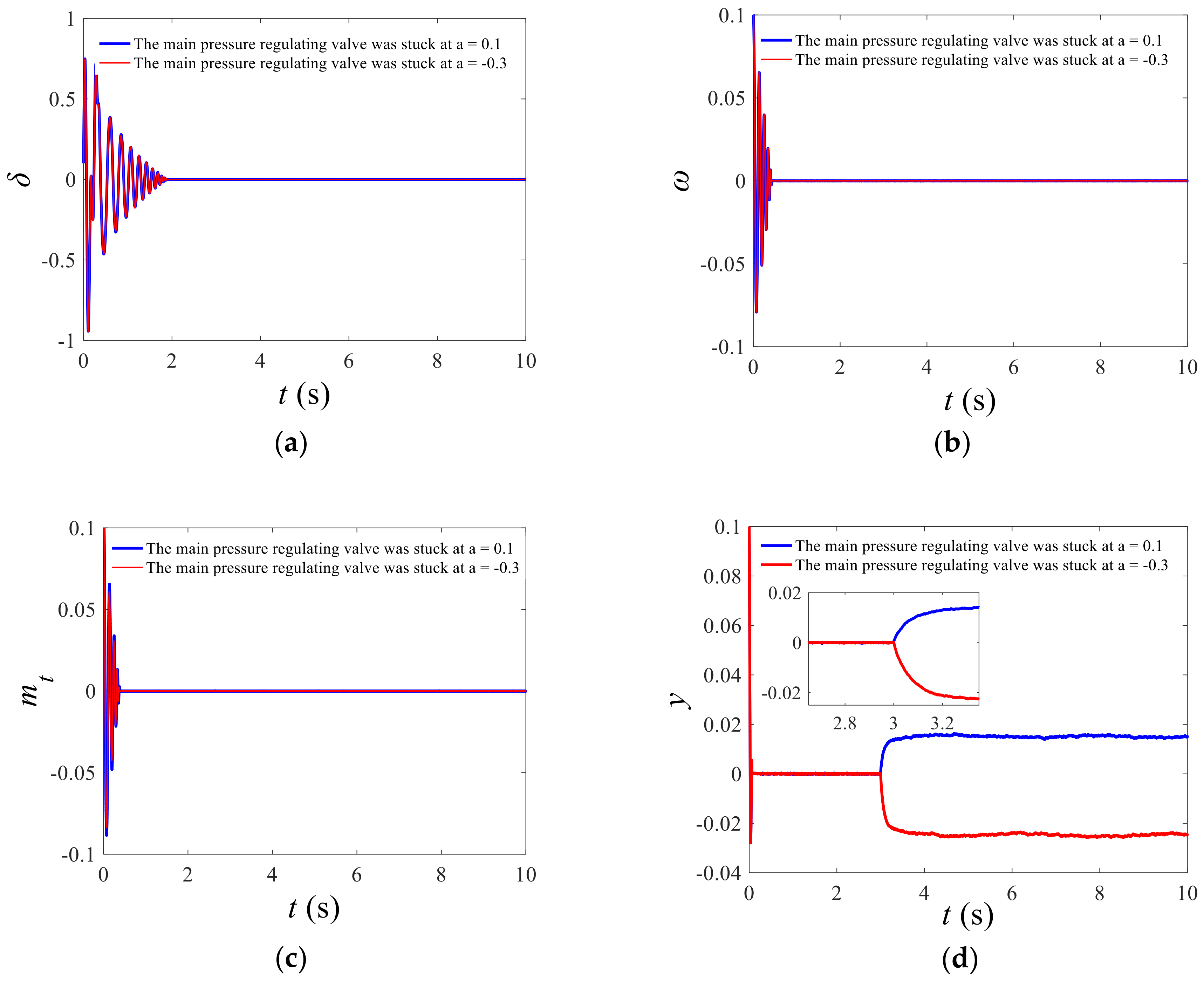
• Case 1: Actuator Lock-in-Place Fault

An actuator lock-in-place fault can be described as $u_i=a_i$, where $a_i$ is a constant and $i=1,2,3,\dots$. The actuator output is limited to $u_{i\min }\le a_i\le u_{i\max }$.

In the electro-hydraulic servo system, a pressure-regulating valve or main relay jam accident is an actuator lock-in-place fault. Figure 3 shows the state trajectories of the HTGS under an actuator lock-in-place fault with the proposed finite-time, fault-tolerant controller (Equation (62)). According to Equation (60), the calculated upper limit of the convergence time was ≈2.18 s. From Figure 3, it is clear that the HTGS could be stabilized and that the slowest response time was the relative deviation of the speed of the generator, which needed ≈2 s (within 2.18 s), verifying the validity of the proposed scheme. It was assumed that the pressure-regulating valve or the main relay could not produce a correct mechanical displacement because of severe wear or jamming from foreign matter. Thus, the vanes could not be operated in accordance with the control signal.

We selected the limit values of the actuator output as $u_{i\min }=-0.1$ and $u_{i\max }=0.1$, and considered two types of actuator lock-in-place faults.

In Figure 3d, it was assumed that at $t=3 \mathrm{s}$, the pressure-regulating valve was stuck in the forward position $a_1=0.1$ and $a_2=-0.3$. As can be seen from the lines in the figure, at $t=3 \mathrm{s}$, despite this fault causing the mechanical displacement to deviate and the relay to move in a single direction, the guide vane finally opened to stabilize at a certain value after $0.3 \mathrm{s}$, and the guide vane opening was stable at $0.015$ and $-0.025$, respectively. More importantly, this degree of deviation could be stabilized to within the feasible operating range $\left[-0.1,0.1\right]$.

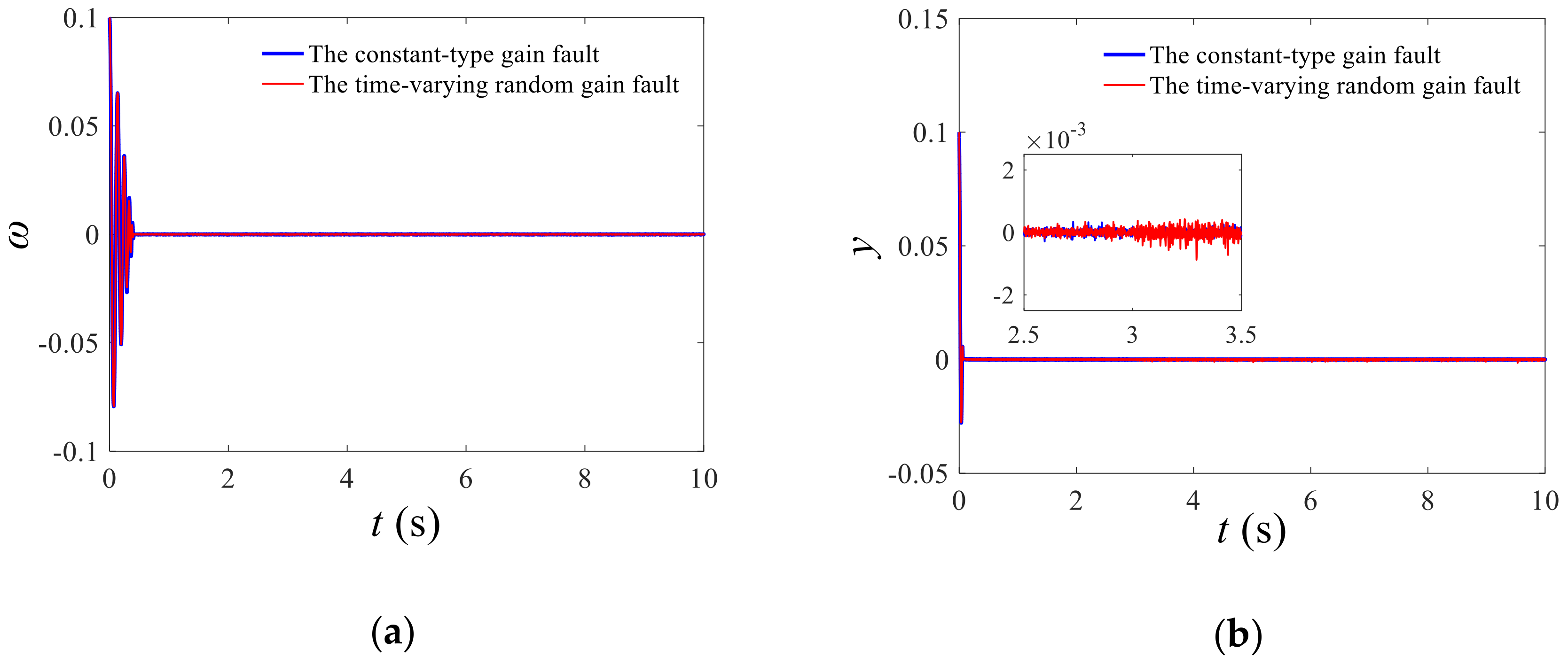
• Case 2: Actuator Constant-Gain Fault

A constant-gain fault is also known as an invalid fault and its fault mode can be described as $u_i=K_i{u}_{pi}$, where $0<K_i\le 1$ is the proportionality factor of the constant gain change, also known as the efficiency factor of the actuator. When $0<K_i<1$, the actuator is still working but the command torque cannot be output; $K_i=0$ means that the actuator is stuck at $u_{i\min }$; and $K_i=1$ means that the actuator is working normally.

This invalid fault often occurs in electro-hydraulic servo systems, e.g., when the leading valve is stuck in an open or closed position for some reason. When the electro-hydraulic converter valve sleeve is stuck, or oil staining or oil temperature causes a zero drift, this may lead to the relay swinging or crawling and the mechanical part clearance may cause partial self-oscillation of the hydraulic automatic system.

Figure 4 shows the state trajectories of the HTGS under an actuator constant-gain fault with the proposed finite-time, fault-tolerant controller (Equation (62)). To further verify the validity of the method used in this paper, we added this failure fault to the actuator, i.e., the guide vane opening. In the constant-gain failure model, $K_i$ is the proportional coefficient of the interval $\left(0,1\right]$. The step function can be used to describe the constant-type fault for the selection of $K_i$. Moreover, sine and cosine functions and random functions can also be used to describe a time-varying random fault of the system.

At $t=3 \mathrm{s}$, the actuator had a constant-value constant-gain fault and a time-varying failure fault. The experimental results are shown in Figure 4b. After $3 \mathrm{s}$ in the experiments here, it was assumed that the system had a constant-value constant-gain fault, $u_{f4}=0.5u_4$ (see the blue line in Figure 4), or a time-varying failure fault, $u_{f4}=\mathrm{rand}\left(1\right)u_4$ (the red line in Figure 4). As can be seen in Figure 4b, after the fault $u_{f4}=\mathrm{rand}\left(1\right)u_4$ was added, the degree of the vane opening fluctuated greatly compared to the steady state, but the minimum and maximum amplitudes did not exceed $0.001$, which was within an acceptable range. In addition, if the added fault is of the constant-type fault $u_{f4}=0.5u_4$, its fluctuation will be very small compared to that of the time-varying faulty system, making it difficult to see the change in the amplitude of the fluctuation. Both experimental results indicate that, under the action of the proposed control method, the system not only had no large fluctuations but also displayed a robust performance.

• Case 3: Actuator Constant-Deviation Fault

The actuator constant-deviation fault mode can be expressed as $u_i=u_{pi}+{\Delta }_i$. In terms of time characteristics, if ${\Delta }_i$ is taken as a constant, it is a constant-type fault; if ${\Delta }_i$ is described using a sine or cosine function, a random function, etc., it is a time-varying random-type fault.

The experimental results shown in Figure 5 are the state trajectories of the HTGS under an actuator constant-deviation fault. From the experimental results, it can be seen that the system state of the hydro-turbine and generator could still be stable by a finite time of $t=2.18 \mathrm{s}$. To verify the validity of the control method, it was assumed that the main pressure-regulating valve changed the frequency signal as a result of electrical regulation or software failure at $t=3 \mathrm{s}$. As a result, the hydraulic pressure was out of balance and the main pressure regulating valve was offset from the equilibrium position.

As can be seen in Figure 5b, when a negative constant-type deviation ${\Delta }_1=-2$ (see the blue lines) or a positive time-varying deviation ${\Delta }_2=2\cos \left(4t\right)$ (see the red lines) occurred, the guide vane opening produced a step in the negative or positive direction at $t=3 \mathrm{s}$. Their amplitudes were ≈$-0.017$ and ≈$0.009$, respectively. It can be seen from the relative ratio of the two lines that the fluctuation of the system caused by a constant-type fault $u_{f4}=2$ was larger than that of the time-varying random-type fault $u_{f4}=-2\cos \left(4t\right)$, and the system fluctuations caused by constant-type faults took longer to dampen. However, no matter what kind of failure, the actuator stabilized after a short period of fluctuation and this time did not exceed $0.05 \mathrm{s}$.

• Case 4: Multiple Actuator Faults

Because of the complexity of the hydroelectric turbine and generator units, there are many reasons why faults are induced. In practice, different types of faults often occur simultaneously. Therefore, when $t=4 \mathrm{s}$, the fault model $u_{f4}=\left|\sin \left(0.6\left(t-1\right)\right)\right|u_4+0.4\cos \left(4t\right)$ was selected for the experiment. Figure 6 shows the state trajectory of multiple actuator faults under the condition of no fault-tolerant control. In Figure 6a, the generator speed relative deviation $\omega$ generated irregular jitters and the jittering tendency gradually became severe. The relative values of the vane opening $y$ in Figure 6b were affected by the fault, which generated periodic fluctuations and the system guide vane was in a swinging state.

.

Figure 7 shows the state trajectories of the HTGS under multiple faults with the proposed fault-tolerant controller (Equation (62)). As seen in Figure 7b, when the electro-hydraulic servo system had both a gain fault and a deviation fault at $t=4 \mathrm{s}$, the guide vane opening was stabilized after a brief shock. However, because the fault model $u_{f4}=\left|\sin \left(0.6\left(t-1\right)\right)\right|u_4+0.4\cos \left(4t\right)$ had a sine function, it can be seen that the added fault appeared to be periodic. After the system stabilized, a fault was generated again after a corresponding period. The controller worked again and stabilized after a short period of oscillation. This behavior continued, but each time, the shock did not exceed 1.5 s (within 2.18 s). The direction and amplitude of each fluctuation were different because there were random disturbances in the system. Therefore, it was shown that the fault estimator designed in this study could accurately estimate the fault signal and displayed a robust performance. Moreover, the reliability of the finite-time, fault-tolerant control was fully shown.

5. Conclusions

In this study, a finite-time, fault-tolerant control method for nonlinear fractional-order HTGSs was studied. By considering external disturbances, such as a stochastic load and an actuator fault resulting from long-term, high-power operation, a fractional-order model for the nonlinear HTGSs with uncertainty, an external disturbance, and an actuator fault was introduced. A finite-time fault estimator was proposed to quickly track the change of the fault signal when an actuator fault occurred. When the actuator failed, the estimator could quickly track the change of the fault signal. The fault estimator could directly act on the controller and guide the controller to make the system state quickly recover to a stable state. Compared with the traditional fault observer, the signal tracking was stable in this way and the reaction time was shorter. A novel sliding surface and a new finite-time, fault-tolerant controller were designed for the fractional-order HTGSs with an actuator fault. The controller incorporated a smooth, bounded arctangent function, which could better suppress system jitters and uncertainty compared with other existing controllers. Therefore, it had better robustness. Finally, based on the different fault models of the hydraulic servo system, numerical experiments were implemented to show the feasibility and fault tolerance of the proposed method.

The designed finite-time, fault-tolerant control could not only ensure the stable operation of an HTGS when a fault occurs but also had acceptable performance indicators. With the continuous deepening of the development of hydraulic resources, the use of HTGS will face increasingly more complex situations. The performance requirements of HTGSs will be more stringent. In the subsequent research, we will pay more attention to the flexibility and time delay effect of HTGSs. In addition, to better grasp the fault form of the actuator, we will aim to integrate fault diagnosis and detection methods to analyze and study the fault-tolerant control of HTGSs.

References

1. Chang, X.L.; Liu, X.H.; Zhou, W. Hydropower in China at present and its further development. Energy 2010, 3, 4400–4406. [Google Scholar] [CrossRef]
2. Shakya, S.R.; Shrestha, R.M. Transport sector electrification in a hydropower resource rich developing country: Energy security, environmental and climate change co-benefits. Energy Sustain. Dev. 2011, 15, 147–159. [Google Scholar] [CrossRef]
3. Stenzel, P.; Linssen, J. Concept and potential of pumped hydro storage in federal waterways. Appl. Energy 2016, 162, 486–493. [Google Scholar] [CrossRef]
4. Frey, G.W.; Linke, D.M. Hydropower as a renewable and sustainable energy resource meeting global energy challenges in a reasonable way. Energy Policy 2002, 30, 1261–1265. [Google Scholar] [CrossRef]
5. Li, X.Z.; Chen, Z.J.; Fan, X.C.; Cheng, Z.J. Hydropower development situation and prospects in China. Renew. Sustain. Energy Rev. 2018, 82, 232–239. [Google Scholar] [CrossRef]
6. Fu, W.L.; Wang, K.; Li, C.S.; Li, X.; Li, Y.H.; Zhong, H. Vibration trend measurement for a hydropower generator based on optimal variational mode decomposition and an LSSVM improved with chaotic sine cosine algorithm optimization. Meas. Sci. Technol. 2019, 30, 015012. [Google Scholar] [CrossRef]
7. Zhang, Y.N.; Chen, T.; Li, J.W.; Yu, J.X. Experimental study of load variations on pressure fluctuations in a prototype reversible pump turbine in generating mode. J. Fluids Eng. 2017, 139, 074501. [Google Scholar] [CrossRef]
8. Xu, Y.H.; Li, C.S.; Wang, Z.B.; Zhang, N.; Peng, B. Load frequency control of a novel renewable energy integrated micro-grid containing pumped hydropower energy storage. IEEE Access 2018, 6, 29067–29077. [Google Scholar] [CrossRef]
9. Guo, R.P.; Zhu, X.J.; Chen, B.; Yue, Y.L. Ecological network analysis of the virtual water network within China’s electric power system during 2007–2012. Appl. Energy 2016, 168, 110–121. [Google Scholar] [CrossRef]
10. Xu, B.B.; Chen, D.Y.; Zhang, X.L.; Alireza, R. Parametric uncertainty in affecting transient characteristics of multi-parallel hydropower systems in the successive load rejection. Int. J. Electr. Power 2019, 10, 444–454. [Google Scholar] [CrossRef]
11. Riasi, A.; Tazraei, P. Numerical analysis of the hydraulic transient response in the presence of surge tanks and relief valves. Renew. Energy 2017, 107, 138–146. [Google Scholar] [CrossRef] [Green Version]
12. Kurzin, V.B.; Seleznev, V.S. Mechanism of emergence of intense vibrations of turbines on the Sayano-Shushensk hydro power plant. J. Appl. Mech. Tech. Phys. 2010, 51, 590–597. [Google Scholar] [CrossRef]
13. Yu, X.D.; Zhang, J.; Fan, C.Y.; Chen, S. Stability analysis of governor-turbine-hydraulic system by state space method and graph theory. Energy 2016, 114, 613–622. [Google Scholar] [CrossRef]
14. Zhang, Y.N.; Zheng, X.H.; Li, J.W.; Du, X.Z. Experimental study on the vibrational performance and its physical origins of a prototype reversible pump turbine in the pumped hydro energy storage power station. Renew. Energy 2019, 130, 667–676. [Google Scholar] [CrossRef]
15. Ren, H.P.; Fan, J.T.; Kaynak, O. Optimal design of a fractional-order proportional- integer-differential controller for a pneumatic position servo system. IEEE Trans. Ind. Electron. 2019, 66, 6220–6229. [Google Scholar] [CrossRef]
16. Zerpa, J.M.; Canelas, A.; Sensale, B.; Santana, D.B.; Armentano, R.L. Modeling the arterial wall mechanics using a novel high-order viscoelastic fractional element. Appl. Math. Model. 2015, 39, 4767–4780. [Google Scholar] [CrossRef]
17. Rasheed, A.; Anwar, M.S. Simulations of variable concentration aspects in a fractional nonlinear viscoelastic fluid flow. Commun. Nonlinear Sci. 2018, 65, 216–230. [Google Scholar] [CrossRef]
18. Yu, W.; Luo, Y.; Pi, Y. Fractional order modeling and control for permanent magnet synchronous motor velocity servo system. Mechatronics 2013, 23, 813–820. [Google Scholar] [CrossRef]
19. Gabano, J.D.; Poinot, T. Fractional modelling and identification of thermal systems. Signal. Process. 2011, 91, 531–541. [Google Scholar] [CrossRef]
20. Flores-Tlacuahuac, A.; Biegler, L. Optimization of fractional order dynamic chemical processing systems. Ind. Eng. Chem. Res. 2014, 53, 5110–5127. [Google Scholar] [CrossRef]
21. Wang, F.F.; Chen, D.Y.; Xu, B.B.; Zhang, H. Nonlinear dynamics of a novel fractional-order Francis hydro-turbine governing system with time delay. Chaos Solitons Fractals 2016, 91, 329–338. [Google Scholar] [CrossRef] [Green Version]
22. Dounis, A.I.; Kofinas, P.; Alafodimos, C.; Tseles, D. Adaptive fuzzy gain scheduling PID controller for maximum power point tracking of photovoltaic system. Renew. Energy 2013, 60, 202–214. [Google Scholar] [CrossRef]
23. Ge, M.; Chiu, M.S.; Wang, Q.G. Robust PID controller design via LMI approach. J. Process. Contr. 2002, 12, 3–13. [Google Scholar] [CrossRef]
24. Chen, Z.H.; Yuan, X.H.; Tian, H.; Ji, B. Improved gravitational search algorithm for parameter identification of water turbine regulation system. Energy Convers. Manag. 2014, 78, 306–315. [Google Scholar] [CrossRef]
25. Wang, B.; Xue, J.Y.; Wu, F.J.; Zhu, D.L. Robust Takagi-Sugeno fuzzy control for fractional order hydro-turbine governing system. ISA. Trans. 2016, 65, 72–80. [Google Scholar] [CrossRef] [PubMed]
26. Liang, J.; Yuan, X.H.; Yuan, Y.B.; Chen, Z.H. Nonlinear dynamic analysis and robust controller design for Francis hydraulic turbine regulating system with a straight-tube surge tank. Mech. Syst. Signal. Pr. 2017, 85, 927–946. [Google Scholar] [CrossRef]
27. Mu, W.Y.; Wang, J.P.; Feng, W.W. Fault detection and fault-tolerant control of actuators and sensors in distributed parameter systems. J. Frankl. Inst. 2017, 354, 3341–3363. [Google Scholar] [CrossRef]
28. Kavikumar, R.; Sakthivel, R.; Kaviarasan, B.; Kwon, O.M.; Anthoni, S.M. Non-fragile control design for interval-valued fuzzy systems against nonlinear actuator faults. Fuzzy Set. Syst. 2019, 365, 40–59. [Google Scholar] [CrossRef]
29. Li, Y.X.; Yang, G.H. Adaptive asymptotic tracking control of uncertain non-linear systems with input quantization and actuator faults. Automatica 2016, 72, 177–185. [Google Scholar] [CrossRef]
30. Joseph, A.; Chelliah, T.R.; Lee, K.B. Multi-channel VSI fed large variable speed asynchronous hydro-condenser: Fault analysis, fault diagnosis and fault tolerant control. IET. Renew. Power Gen. 2019, 13, 438–450. [Google Scholar] [CrossRef]
31. Wang, J.H.; Gao, Y.B.; Qiu, J.B.; Ahn, C.K. Sliding mode control for non-linear systems by Takagi-Sugeno fuzzy model and delta operator approaches. IET. Control. Theory Appl. 2017, 11, 1205–1213. [Google Scholar] [CrossRef]
32. Tin, Z.Y.; Luo, J.J.; Wei, C.S. Quasi fixed-time fault-tolerant control for nonlinear mechanical systems with enhanced performance. Appl. Math. Comput. 2019, 352, 157–173. [Google Scholar]
33. Wang, B.; Xue, J.Y.; Wu, F.J.; Zhu, D.L. Finite time takagi-sugeno fuzzy control for hydro-turbine governing system. J. Vib. Control 2018, 24, 1001–1010. [Google Scholar] [CrossRef]
34. Guo, Q.; Wang, Q.; Li, X.C. Finite-time convergent control of electrohydraulic velocity servo system under uncertain parameter and external load. IEEE Trans. Ind. Electron. 2019, 66, 4513–4523. [Google Scholar] [CrossRef]
35. Wang, F.; Chen, B.; Sun, Y.M.; Lin, C. Finite time control of switched stochastic nonlinear systems. Fuzzy Set. Syst. 2019, 365, 140–152. [Google Scholar] [CrossRef]
36. Podlubny, I. Fractional Differential Equations; Academic Press: New York, NY, USA, 1999. [Google Scholar]
37. Li, Y.; Chen, Y.Q.; Podlubny, I. Mittag-Leffler stability of fractional order nonlinear dynamic systems. Automatica 2009, 45, 1965–1969. [Google Scholar] [CrossRef]
38. Kilbas, A.; Srivastava, H.M.; Trujillo, J.J. Theory and Applications of Fractional Differential Equations, 1st ed.; Elsevier Science: Amsterdam, The Netherlands, 2006. [Google Scholar]
39. Samko, S.; Vakulov, B. Weighted Sobolev theorem with variable exponent for spatial and spherical potential operators. J. Math. Anal. Appl. 2005, 310, 229–246. [Google Scholar] [CrossRef] [Green Version]
40. Samko, S.G.; Kilbas, A.A.; Marichev, O.I. Fractional Integrals and Derivatives: Theory and Applications; Gordon and Breach Science Publishers: Yverdon, Switzerland, 1993. [Google Scholar]
41. Ling, D.J. Bifurcation and Chaos of Hydraulic Turbine Governor; Hohai University: Nanjing, China, 2007. [Google Scholar]
42. Efe, M.O. Fractional fuzzy adaptive sliding-mode control of a 2-DOF direct-drive robot arm. IEEE Trans. Syst. Man Cybern. B 2008, 38, 1561–1570. [Google Scholar] [CrossRef]
43. Peng, B. Fault Diagnosis of Hydroelectric Generating Units Based on Improved Support Vector Machine and Feature Information Fusion; Huazhong University of Science & Technology: Wuhan, China, 2008. [Google Scholar]
44. Zhang, P. Research on Fault Detection and Diagnosis of Hydraulic Turbine Control System; Xi’an University of Technology: Xi’an, China, 2006. [Google Scholar]
Figure 1. Structure of the main pressure regulating valve. (a) Sketch of the main pressure-regulating valve; (b) Diagram of the main pressure valve structure.
Energies 13 03812 g001aEnergies 13 03812 g001b
Figure 2. State trajectories of the hydraulic-turbine-governing system (HTGS) without a controller. (a) δ t t ; (b) ω t t ; (c) m t t t ; (d) y t t .
Energies 13 03812 g002
Figure 3. State trajectories of the HTGS under an actuator lock-in-place fault. (a) δ t t ; (b) ω t t ; (c) m t t t ; (d) y t t .
Energies 13 03812 g003
Figure 4. State trajectories of the HTGS under an actuator constant-gain fault. (a) ω t t ; (b) y t t .
Energies 13 03812 g004
Figure 5. State trajectories of the HTGS under an actuator constant-deviation fault. (a) ω t t ; (b) y t t .
Energies 13 03812 g005
Figure 6. State trajectories of the HTGS under multiple faults without fault-tolerant control. (a) ω t t ; (b) y t t .
Energies 13 03812 g006
Figure 7. State trajectories of the HTGS under multiple faults with the proposed fault-tolerant controller (Equation (62)). (a) ω t t ; (b) y t t .
Energies 13 03812 g007