Abstract
This study aims to test the effects of changes in international crude oil prices on changes in crude oil and hydropower use from 1965 to 2016. We suggest a cointegration relationship between the consumption of coal, crude oil, and hydropower and the real crude oil price. The real price is weakly exogenous for the long-run relationship and has impacted energy consumption accordingly. The long-run crude oil price elasticity of oil use is 0.460. Our estimate suggests a positive oil price–oil use relationship in China, which is dramatically different from many previous studies but is consistent with a few past studies. The growth in external oil prices may lead to a long-run increase in hydropower use in China, with a long-run price elasticity of 0.242. The long-run crude oil price elasticity of coal use is −0.930. Hence, increased oil and hydropower use could make up the energy supply–demand gap left over by the decreased coal use. Strictly planned domestic fuel prices and rapidly growing family incomes should diminish the negative effect of external oil prices on domestic crude oil demand. In the long run, given a strictly managed energy price, the growth in external oil prices is not likely to noticeably restrain the domestic oil demand or lead to a dramatic increase in coal use. We suggest that the large-scale development and utilization of hydropower may be inappropriate. Coal utilization policies must be reviewed. The appropriate increase in clean coal consumption could reduce the consumption of crude oil and hydropower; meanwhile, carbon emissions will not increase.
1. Introduction
In 2006, the use of coal, crude oil, natural gas, and non-fossil energy (hydropower, nuclear, and wind power as a whole) accounted for 72.4%, 17.5%, 2.70%, and 7.40%, respectively, of China’s total primary energy consumption. To build a sustainable energy use structure, China has since enacted the 11th, 12th, and 13th Five-Year Plans for Energy Development (PED) [1,2,3].
The overall energy use policy is that in the coming decade, China must significantly reduce the proportion of coal consumption and adequately reduce the percentage of crude oil consumption, while substantially increasing the share of natural gas and non-fossil energy consumption. By 2015, the shares of coal, crude oil, natural gas, and non-fossil use were targeted to be 65%, 16.1%, 7.5%, and 11.4%, respectively. In fact, by 2016, the proportion of coal use had declined significantly to 62.0%, achieving the planned target. The portions of natural gas and non-fossil use were 6.40% and 13.3%, respectively [4], so the non-fossil energy use share exceeded the planned target.
Nevertheless, the share of crude oil did not decline as required by the PEDs; instead, it grew to 18.3% in 2016 and further to 18.9% in 2018. One issue arising from the change in the share of oil use is whether external crude oil prices are a determinant of the domestic demand for crude oil in China, as China’s dependence on foreign markets to meet the demand for oil has been substantial. Although China produced 271.44 million tons of coal equivalent (Mtce) of crude oil in 2018, it consumed 876.96 Mtce; hence, 69.2% of the nation’s oil consumption depended on imports [4]. Moreover, its crude oil imports accounted for 15.5% of the world’s exports in 2018 [5].
Since 1965, international crude oil prices have fluctuated (Figure 1) [6]. Baffes and Kshirsagar (2016) noted four oil price crashes for the period 1983 to 2016 [7]. These crashes might have stimulated the increase in China’s oil consumption and accordingly had a permanent effect on oil use. Usually, there is a negative relationship between crude oil prices and economic activity [8], with oil prices preceding the economy [9,10]. Hamilton (1988) suggested that oil price increases may cause consumers or firms to postpone purchases of energy-intensive equipment until there is greater certainty about energy costs, with a resulting decline in demand for capital goods and consumer durables leading to a recession [11]. Moreover, rising oil prices may cause a shock to the supply side and accordingly reduce potential output [12]. One example is that the increase in energy prices significantly decreased China’s industrial output and thereby reduced oil (product) consumption [13].
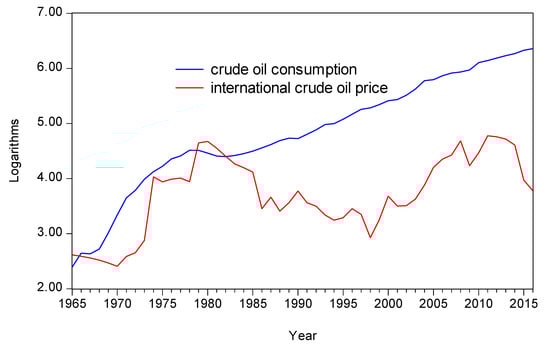
Figure 1.
Change in crude oil price and consumption in China.
However, from 1999 to 2010, oil use increased with rising oil prices. Considering the transportation sector as an example, Zou and Chau (2019) argued that because government-controlled energy prices distorted market fuel prices [14], freight demand in various modes of freight transportation considered fuel prices less than it would have otherwise. Therefore, although freight transportation is an energy-intensive sector [15], whether in the short or long run, real fuel prices did not influence freight transportation volumes and, accordingly, the consumption of oil products [16]. The effect of global oil prices on oil use in China is mixed, and thus an examination of their long-run relationship is significant.
The effect of global crude oil prices on demand for a nation’s oil and other types of energy is an empirical issue. Thus, this study mainly aims to examine the effect of (real) world crude oil prices on the consumption of coal, crude oil, natural gas, and hydropower in China. This paper contributes to the literature mainly in three aspects. We distinguish between the short- and long-run effects of price, as the latter is economically very significant. We suggest a positive long-run oil consumption–oil price relationship. We also suggest a weak exogeneity of international crude oil prices for the long-run relationship. In addition, this paper finds that whether in the short or long run, oil use is price inelastic, which supports past studies.
The remainder of this paper is organized as follows. Section 2 is a literature review. Section 3 introduces the methods applied. Section 4 addresses the time series of data. Section 5 reports the estimated results. Section 6 is a discussion focusing on the long-run relationship, and Section 7 concludes the paper.
2. Literature Review
In a rationally expected market, energy demand changes with energy prices and vice versa. Whether or not energy prices impact energy demand is often an econometric issue. In terms of causal links, energy (fuel) prices influence energy consumption. For example, in the long run, the real oil price influences nuclear energy consumption in the US, Japan, Canada, and Germany. In the short run, it Granger-causes nuclear energy consumption [17]. Energy consumption, energy prices, and income are mutually causal in the short run. Thus, they are not neutral with respect to each other [18]. In the oil-dependent Ecuadorean economy, crude oil prices Granger-caused energy consumption but not vice versa [19]. However, energy prices have little effect on energy consumption, which is attributed to the energy price mechanism that is more government-oriented than market-oriented [20].
The extent of long-run price elasticity of energy use might be greater than that in the short run due to the time lag required to respond to a price shock [21]. Labandeira et al. (2017) also found that the average short- and long-run price elasticities of overall energy demand were –0.149 and –0.570, respectively [22].
In the US, the short- and long-run price elasticities of crude oil consumption per capita were −0.061 and −0.453, respectively; in the UK, they were −0.068 and −0.182; and in Japan, they were −0.071 and −0.357 [21]. The mean short- and long-run price elasticities of the demand for gasoline were −0.34 and −0.84, respectively [23].
On the other hand, energy use also positively responds to changes in energy prices [24]. The reason may be that increasing crude oil prices have been found to create economic conditions that produce more energy consumption in the economy [19].
In India, over the period from 1971–2015, real income, commercial energy use per capita, and energy prices were cointegrated [25]. In South Africa, imported crude oil, price, and income were cointegrated, with the long-run price and income elasticities of imported crude oil being 0.147 and 0.429, respectively. Overall, gasoline demand, price, and income were cointegrated, with the price and income elasticities of gasoline demand for 1978–2005 being −0.47 and 0.36 [26].
China’s average short- and long-run price elasticities of crude oil consumption per capita over 1979–2000 were 0.001 and 0.005, respectively [21]. Chai et al. (2016) suggested that the West Texas Intermediate (WTI) price elasticity of crude oil consumption from 1987–2014 in China was 0.153.
3. Methodology
This study argues that international crude oil prices can be a determinant of domestic primary energy consumption in China and, accordingly, supply dynamics for the changes in overall energy use structure. The cointegration theory takes all time series variables in an economic system as endogenous a priori [27]. To examine the relationship between energy consumption and oil prices, we tested for cointegration using the Engle–Granger test [27] and the Johansen trace test [28,29]. The Johansen test applies the following vector autoregressive model (VAR):
where yt is a set of I(1) variables, μ denotes the intercept, k denotes the lag order, and Dt is the seasonal dummy. εt is white noise with zero mean and finite variance. The null hypothesis of at most r cointegration vectors is tested using the maximum likelihood estimation (MLE) method. The likelihood ratio (LR) test statistic is called the trace statistic.
The Johansen test estimates . The cointegration vector β represents the long-run relationship, within which long-run elasticities can be inferred. α is the adjustment coefficient for β, which reflects the short-run dynamics that variables impose on the long-run system. By imposing a zero restriction on α, we tested for the weak exogeneity of a variable for the long-run relation. Weak exogeneity implies a long-run effect on the system, thus economic significance [30,31,32,33,34].
Moreover, cointegration implies a valid linear error-correction model (ECM) between I(1) variables. Super-consistency of cointegration allows us to incorporate cointegrating vector β into a conventional VAR to formulate an ECM, which can lead to optimal inferences [35]. Despite this, a first-differenced VAR is still valid for an I(1), but not a cointegrated, variable set [27].
Working with the estimated ECM, we conducted the Granger causality test using the Wald χ2-statistic and the LR test. In small samples, the LR test outperforms the Wald F-test in terms of size and power [36].
We tested for unit roots using the augmented Dickey–Fuller (ADF) [37], Phillips–Perron (PP) [38], and Elliott–Rothenberg–Stock modified Dickey–Fuller (ERS DF) [39] tests. The ERS DF test can work well in small samples; particularly, if this test applies generalized least squares (GLS) to de-trend data and selects the lag length using a modified Akaike information criterion (MAIC), the test will have less loss of power and a preferable size [40]. We applied the ERS DF test along with the MAIC (i.e., the ERS DF-GLS test).
All the means in our dataset are non-zero. Variables appear to move upwards over time, which implies a trend. In such cases, the Perron test uses the innovational outlier (IO) model C to test for a structural break. The Perron structural break test allows for both level and slope shifts taking place simultaneously. It rejects the null hypothesis of a unit root more frequently than the Zivot–Andrews test [41,42,43]. Sen recommended model C when the break date is taken as unknown [44]. The Perron technique can suggest only one structural change. Multiple trend breaks have been suggested [45,46]. We estimated the following Perron IO model C:
where DUt allows for a one-time change in the intercept of the trend function and DUt = 1 if t > Tb and 0 otherwise; T denotes the sample size, and Tb is the break date to be selected; DTt allows for a change in the slope of the trend function and DTt = t if t > Tb and 0 otherwise; and D(Tb), the one-time dummy, equals 1 if t = Tb + 1 and 0 otherwise.
The tα value on α is used to evaluate the null hypothesis. Under the null hypothesis of a unit root, (except in model C), , , and . , and it should be significantly different from zero. Under the alternative hypothesis of a trend stationary process, , , (in general), , and .
4. Data
Yearly global crude oil prices and primary energy consumption in China came from the Statistical Review of World Energy 2017. British petroleum (BP) has published the Statistical Review of World Energy since 1951 [6]. It is worth pointing out that yearly and monthly primary energy consumption data before 2000 are not available from the National Bureau of Statistics of China (NBSC) [4]; data cover the period 1965 to 2016. Crude oil prices are measured in US dollars per barrel and were deflated using the 2016 US consumer price index (CPI). We defined the following variables.
- ENERGY: Total energy consumption
- COAL: Coal consumption
- OIL: Crude oil consumption
- HYDRO: Hydropower consumption
- GAS: Natural gas consumption
- PRICE: Real crude oil price
The data have non-zero means (Table 1). All types of energy consumption have trended upwards over time. Real crude oil prices appear to have markedly fluctuated throughout the entire study period (Figure 2). Hence, the data implicitly contain constants and trends.

Table 1.
Descriptive statistics of the data.
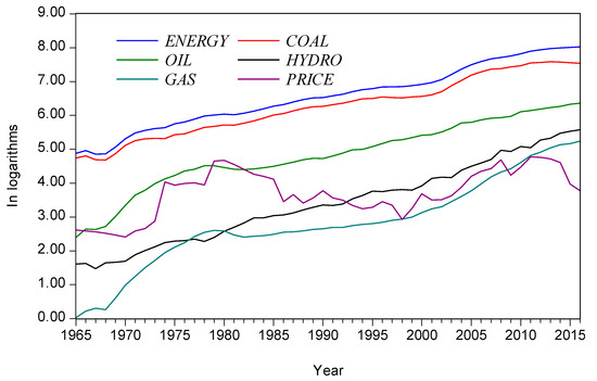
Figure 2.
Real international crude oil prices and energy consumption in China.
Jarque-Bera statistics show that we can accept the normality for ENERGY, COAL, and OIL at the 1% level, and for PRICE at the 5% level. However, we reject the normality for GAS and HYDRO at the 1% level; these two variables contain a kurtosis that exceeds 3.0, which may indicate an outlier in the data. Despite this, the logarithms of data have a kurtosis below 3.0 (2.82 for GAS and 1.97 for HYDRO). Hence, the logarithms of data improve the data quality.
5. Empirical Results
5.1. Break Dates
Table 2 reports the Perron tests. Based on the finite-sample critical value in Perron (1997), we accepted the null hypothesis of a unit root for the variables PRICE, OIL, and HYDRO at the 10% level, and the null hypothesis for the variable COAL at the 1% level. Thus, these four variables contained a unit root. We rejected the null hypothesis for ENERGY and GAS at the 1% level, which indicates that they both contained a structural break. The break for total energy consumption (ENERGY) occurred in 1981. The break for natural gas consumption (GAS) occurred in 2000.
Table 2.
Break date tests using the Perron innovational outlier (IO) model C.
5.2. Unit Root
For ENERGY, the ADF, PP, and ERS DF-GLS tests consistently indicated a unit root. Moreover, in the Perron test, , , and (0.76), which implied a unit root. However, ≠ 0 and , which implied a trend stationary process. Hence, we took ENERGY as an I(1) process with a break that occurred in 1981.
For COAL, the ADF, PP, and ERS DF-GLS tests indicated a unit root. Moreover, the Perron test implied a unit root. Hence, we took COAL as an I(1) process.
For OIL, both the PP and ERS DF-GLS tests indicated that it had a unit root, but the ADF test indicated that it was stationary. Furthermore, the Perron test suggested a unit root. Hence, we took OIL as a near I(1) process.
For GAS, the ADF and ERS DF-GLS tests indicated that it contained at least two unit roots, while the PP test indicated two unit roots. Moreover, the Perron test suggested a structural shift. Hence, we took GAS as a nonstationary process with at least two unit roots.
For HYDRO, the PP and ERS DF-GLS tests indicated that it had a unit root, but the ADF test indicated two. Moreover, the Perron test implied a unit root. Hence, we took HYDRO as a near I(1) process.
For PRICE, the ADF and PP tests indicated that it had a unit root (Table 3). However, the ERS DF-GLS test indicated at least two. Moreover, the Perron test suggested a unit root in PRICE even at the 10% level. Hence, we took PRICE as a near I(1) process.
Table 3.
Unit root tests.
Overall, we suggested that each of the five variables, PRICE, ENERGY, COAL, OIL, and HYDRO, contained a unit root. In addition, ENERGY contained a breakpoint and GAS contained a breakpoint and at least two unit roots.
5.3. Cointegration Analysis
We removed the natural gas consumption variable (GAS) from the subsequent analysis because it had at least two unit roots. In addition, we removed the total energy consumption variable (ENERGY) from the cointegration to avoid any possible effect arising from the structural break (an outlier). Hence, we tested for cointegration among the remaining four variables: COAL, OIL, HYDRO, and PRICE.
5.3.1. Engle–Granger Test
As Figure 2 indicates, the data appeared to grow over time and have non-zero means. Hence, test equations contained both a constant and a linear trend. When PRICE was taken as a dependent variable, the null hypothesis of no cointegration was rejected at the 5% level (Table 4). When OIL, COAL, and HYDRO were taken as dependent variables, the null hypothesis was accepted at the 5% level.
Table 4.
Engle–Granger test.
5.3.2. Johansen Tests
Assumptions I, II, III, IV, and V are proposed for the trace statistic. Figure 2 indicates that the data may include the trend and intercept. Hence, we used assumption IV, which is a general case [52].
The Johansen test results are very sensitive to the lag order [53]. A small lag would lead to substantial size distortions and too many cointegration vectors, whereas overparameterization would mean a loss of power [54,55,56].
First, we applied the Johansen test using lag values of 3, 4, 5, 6, 7, and 8. Then, after taking into account the log likelihood, Akaike information criterion (AIC), Schwarz information criterion (SIC), normality, and autocorrelation, we selected an optimal lag length k = 6 (Table 5).
Table 5.
Specification experiments for Johansen cointegration test using different lag values.
All cases passed the multivariate normality test. For the k = 3 case, the long-run price elasticity of hydropower use was negative, which may not be plausible. Moreover, autocorrelations existed at the 10% level. For the k = 4 case, the short-run price elasticity of crude oil use contained a positive sign, which also may not be plausible. For the k = 7 case, the short-run price elasticity of crude oil consumption was statistically insignificant; there was a very high (negative) price elasticity of coal use (−2.86). The k = 8 case had the largest log likelihood and the smallest AIC and SIC; with positive signs, the short-run price elasticity (0.77) of crude oil consumption was greater than the long-run (0.65). In addition, there was an excessively high (negative) price elasticity of coal use, which implies that with growing crude oil prices, coal use declined substantially, which has rarely occurred in China.
Regarding the k = 5 and 6 cases, they had similar short-run and long-run price elasticities of crude oil use and coal and hydropower use. However, the k = 6 case had a greater log likelihood and smaller AIC and SIC than the k = 5 case. Hence, we selected the k = 6 case for the final Johansen test.
Asymptotically, trace tests suggested four cointegration relations at the 5% level (Table 6). Nonetheless, both the Cheung–Lai critical value and Reinsel–Ahn trace corrections suggested one cointegration relation. Hence, we suggest that there is only one cointegrating vector.
Table 6.
Johansen cointegration test.
The normalized cointegrating vector β can be written as follows:
where t-statistics are in parentheses. Equation (3) indicates that all estimated coefficients and time trends are statistically significant. The estimated coefficients are interpreted as the long-run elasticity. Hence, the long-run price elasticities of the consumption of coal, crude oil, and hydropower are −0.930, 0.460, and 0.242, respectively.
5.4. Weak Exogeneity Tests
By imposing a zero restriction on α, we conducted LR tests for the weak exogeneity of variables for the estimated long-run relationship (Table 7). At the 1% level, we rejected the null hypothesis of weak exogeneity for COAL, OIL, and HYDRO, whereas we accepted the null hypothesis at the 10% level for PRICE. Hence, real crude oil prices have driven the long-run equilibrium and, accordingly, influenced various types of energy consumption.
Table 7.
Weak exogeneity test.
5.5. ECM Estimation and Granger Causality Test
The Granger representation theorem shows that cointegration implies an ECM model and at least a unidirectional Granger causality between variables of interest [27]. We estimated an ECM matrix (Table 8) and conducted the Granger causality test within these ECMs.
Table 8.
Estimates of error-correction models (ECMs).
Table 9 reports the results of the Granger causality test using both the LR and Wald χ2 tests. The existence or nonexistence of a causal relationship is based on the consistency of these two tests. Hence, PRICE Granger-caused COAL, as the LR rejected the null hypothesis at the 1% level, while the Wald-χ2 test rejected the null hypothesis at the 5% level. PRICE Granger-caused OIL and HYDRO, as both the LR and Wald χ2 tests rejected the null hypothesis at the 1% level. Conversely, OIL Granger-caused PRICE, as the LR rejected the null hypothesis at the 1% level, while the Wald χ2 test rejected the null hypothesis at the 5% level.
Table 9.
Granger causality test.
Overall, real crude oil prices Granger-caused the consumption of coal, crude oil, and hydropower. Oil consumption Granger-caused crude oil prices. Regarding the short-run effects of crude oil prices on coal consumption in the estimated ECM, the first and fourth lagged terms are statistically significant, with the absolute values of the t-statistics being greater than or equal to 2.00, and the estimated coefficients of these two terms are 0.254 and 0.167, respectively. Hence, oil prices positively and slightly influenced coal consumption; the (average) short-run (in four years) price elasticity of coal consumption is about 0.211.
Similarly, oil consumption negatively and slightly responded to the change in oil prices; the (average) short-run (in five years) price elasticity of oil use is −0.182. Oil prices negatively and slightly influenced hydropower consumption; the (average) short-run (in four years) price elasticity of hydropower consumption is −0.421. In addition, a 1% growth in oil consumption in China could mean a growth in international oil prices of 4.80% in the short run (three years), which reflects a substantial short-run effect of China’s oil use on external prices.
6. Discussions
Empirical results suggest that in the long run, real crude oil prices and the consumption of coal, crude oil, and hydropower tend to move together. There is a positive long-run crude oil use–price relationship; however, there is a negative long-run coal demand–oil price relationship. The estimated long-run price elasticities of the consumption of coal, crude oil, and hydropower are −0.930, 0.460, and 0.242, respectively. The dynamics of the long-run energy consumption linkage may primarily come from the oil price, as it is weakly exogenous for the long-run relationship.
We find that energy consumption and energy (crude oil) prices have a long-run relationship. This finding is consistent with many previous studies, including [17,21,22,23,25,26].
The estimated long-run price elasticity of crude oil use was 0.460 from 1965 to 2016. Our estimate suggests the positive linkage between world oil prices and oil consumption in China, which is consistent with a few past studies. For example, the average long-run price elasticity of crude oil consumption per capita was 0.005 for the 1979–2000 period [21], and the WTI price elasticity of crude oil consumption was 0.153 for the 1987–2014 period [24]. It is noteworthy that the long-run price elasticity of imported crude oil was 0.147 from 1978–2005 in South Africa [26].
Nevertheless, the positive oil price–oil use relationship in China dramatically differs from the negative long-run price linkage [21,22,23,26]. The literature shows that the average long-run price elasticity of overall energy demand is −0.570 [22]. In the US, the UK, and Japan, the long-run price elasticities of crude oil consumption per capita were −0.453, −0.182, −0.357, respectively [21]. Energy prices in these three developed economies are market-oriented: They seldom decide the price of fuel (gasoline and diesel) by adopting various administrative tools; hence, oil prices and consumption exhibit an inverse relationship. The mean long-run price elasticity of gasoline demand was −0.84 [23]. In South Africa, the price elasticity of gasoline demand for the period from 1978–2005 was −0.47 [26].
Considerable oil imports and strictly controlled energy (fuel) prices in China may explain the positive price effect. Increasing crude oil prices have been found to create economic conditions that produce more energy consumption in the economy [19]. Energy prices have an insignificant effect on energy consumption, which is attributed to the energy price mechanism, which is more government-oriented than market-oriented [20].
China’s overall energy use structure policy may partially account for this positive relationship. The policy required that by 2016, China had to have significantly reduced the proportion of coal consumption and appropriately reduced the proportion of crude oil consumption [1,2,3]. Local governments and energy-intensive firms were under increasing pressure to reduce coal use. Consequently, by 2016, the proportion of coal consumption declined dramatically to 62.0% [4], meeting the target set by the five-year PEDs. Simultaneously, there was a negative long-run elasticity (−0.930) of coal use relative to changes in crude oil prices. However, a wide fuel supply–demand gap was left over by the noticeable reduction of coal use, in terms of both share and quantity. The gap has to be made up by increasing oil use. Thus, the crude oil share has grown markedly since 2006, reaching 18.9% in 2018, which contributes to some extent to a positive long-run crude oil use–price relation. Oil consumption did not experience a structural break. Hence, although there were four price crashes between 1983 and 2016 [7], it seems that these crashes did not permanently shock China’s oil use.
The economy has expanded over the past decade, which means a rapidly growing demand for crude oil, resulting in 69.2% of the nation’s oil consumption depending on imports. During the 2005–2016 period, China’s GDP at constant prices grew by 166.3% [62], while its oil use grew by 71.5% [4]. Expanding crude oil use has resulted from considerable industrial output, real estate production, and a growing number of vehicles, as suggested in [13,16].
Changes in long-term strictly managed energy (or oil product) prices are rarely consistent with changes in external crude oil prices [14,20]. Hence, managed or planned fuel prices could, to a large extent, reduce the negative effect of external oil prices on domestic oil demand. A recent study examined the asymmetric effect of increases and decreases in international oil prices on wholesale prices of gasoline and diesel fuel in China [63]; it suggests that consumers will rarely adjust their consumption of various oil products based on changes in external crude oil prices.
Another explanation for the positive crude oil use–price relationship and the negative coal use–oil price relationship is the substitution of more efficient energy for less efficient energy due to the decline in clean energy prices. Growth in family incomes implies a price decline for fuel, because it can reduce a family’s sensitivity to increases in product prices. Hence, in 20 OECD countries throughout 1980–2010, with the growth in income, oil, and gas use increased, but coal consumption declined [64]. Between 2000 and 2012, urban and rural families’ per capita disposable income in China grew by 287.5% and 267.6%, respectively [65], potentially reducing their sensitivity to higher fuel prices while increasing their consumption of oil products.
In the short run, Granger causality runs from real crude oil prices to the consumption of coal, crude oil, and hydropower. Oil price positively impacts coal use, whereas it negatively influences both crude oil and hydropower consumption. We suggest that the short-run oil price elasticities of crude oil and hydropower consumption are −0.182 and −0.421, respectively, and the short-run oil price elasticity of coal consumption is 0.211. Hence, the main types of primary energy consumption in China are crude oil price-inelastic. The proposed short-run price elasticity of oil consumption in China is very close to the average short-run price elasticity (−0.185) of energy demand among the world’s net energy importers [22]; however, it is much higher than a previous short-run price elasticity estimation (0.001) of crude oil consumption per capita over the 1979–2000 period [21].
The estimated short-run crude oil price elasticity of oil use (−0.182) is very close to the average short-run price elasticity of energy demand by a previous cointegration analysis and ECM simulation (−0.181). In addition, it is close to the average short-run price elasticity of energy demand during the post-1973 period (−0.183) and in net energy importers (−0.185) [22].
Interestingly, the adjustment coefficients on COAL, OIL, HYDRO, and PRICE are −0.22, −0.17, 0.61, and 0.51, respectively. Therefore, the short-run dynamics of coal and oil use need to adjust downwards to return to the long-run equilibrium, suggesting that coal and oil have been excessively consumed. The hydropower use variable needs to adjust upwards for the long term, which implies that there is potential for more hydropower use in terms of optimizing the energy use structure. However, the excessive use of hydropower may produce potential social, economic, and environmental problems (e.g., [66]).
The significant finding is that in the long run, with the rise in international crude oil prices, although China’s crude oil and hydropower consumption have increased, coal consumption has significantly decreased. Therefore, the problem is that the rise in prices cannot suppress the rise in crude oil consumption and, to some extent, promotes the rise in hydropower consumption.
Total energy consumption is still enormous. To significantly reduce carbon emissions, China must drastically reduce coal consumption and encourage the development and consumption of renewable energy [67,68,69]. Hydropower is one of the most important renewable energy sources. From our estimate, an increase in hydropower consumption is accompanied by an increase in coal consumption. The large-scale development of hydropower and rising hydropower consumption have brought ecological and migration problems in China. In addition, increasing hydropower utilization has rarely replaced coal consumption, thereby contributing considerably to the reduction of carbon emissions [66,70,71]. Therefore, we suggest that it is not appropriate to continue to encourage large-scale development and utilization of hydropower.
Due to the expanding economy in the past four decades, rapidly increasing household income, and a large number of vehicles, an enormous consumption of crude oil has made its consumption insensitive to price. Although international crude oil prices have been declining since 2014, the price of fuel oil, such as gasoline and diesel, in China has been rising and has not restrained the increase in crude oil consumption. Therefore, we believe that the policy of relying on increasing oil prices to curb China’s crude oil consumption has failed. To curb the excessive and rapid growth of crude oil consumption, additional taxes and administrative measures may be required. In particular, in the case of substantial total energy consumption, coal utilization policies must be reviewed. Over the past two decades, the proportion of China’s coal utilization in the primary energy structure has reduced significantly. We argue that China may have excessively suppressed coal consumption. We suggest that if investment in coal production and processing increases, and China uses more advanced clean coal technologies, the appropriate increase in clean coal consumption can reduce crude oil and hydropower consumption, and meanwhile, carbon emissions will not increase.
7. Conclusions
China has consumed an enormous amount of crude oil and depended heavily on oil imports. The energy use structure policy requires growth in non-fossil energy and hydropower use, while significantly reducing coal and oil use. Since 2006, the share of coal use has declined, and the shares of crude oil, natural gas, and hydropower use have increased. We argue that changes in international crude oil prices have imposed dynamics on the adjustments of China’s primary energy consumption. Thus, we tested for the long- and short-run effects of the real crude oil price on the consumption of coal, crude oil, and hydropower. The data are annual changes covering the period from 1965 to 2016.
The study suggests a long-run equilibrium relationship between real crude oil prices and the consumption of coal, oil, and hydropower. The price is weakly exogenous for the long-run relationship, implying that oil price has a long-run effect on various types of energy use. The estimated long-run price elasticities of the consumption of coal, oil, and hydropower are −0.930, 0.460, and 0.242, respectively.
Our estimate suggests the positive linkage between world oil prices and oil consumption in China. The noticeable reduction of coal use, a rapidly growing demand for crude oil and heavy dependence on oil imports, and strictly-controlled energy (fuels) prices may be attributable to the positive price effect. Another explanation for the positive relationship may be the substitution of more efficient energy for less efficient energy due to the decline in clean energy prices.
China’s overall energy use policy requires a marked reduction of coal use, which has placed enormous pressure on local governments and coal-intensive firms. The share of coal use has declined, resulting in an energy supply–demand gap. We suggest that this gap has to be made up by increased oil use. Meanwhile, the government has encouraged more development and the use of hydropower. Therefore, hydropower use will positively respond to the real oil price in the long run.
Overall, whether in the long run or the short run, oil use is price-inelastic. In the long run, given a strictly managed energy price, the increase in external oil prices is not likely to noticeably restrain the growth in domestic oil use.
The problem is that the rise in prices cannot suppress the rise in crude oil consumption and, to some extent, promotes the rise in hydropower consumption. We suggest that it is not appropriate to continue to encourage large-scale development and use of hydropower. China may have excessively suppressed coal consumption. The appropriate increase in clean coal consumption could reduce crude oil consumption and hydropower consumption; meanwhile, carbon emissions will not increase. Tests did not include the natural gas variable due to its unit root property. Further examination may employ a longer data period. We acknowledge that multiscale and nonlinear analyses between alternative energy markets and between oil prices and other variables can provide further evidence for a better understanding of changes in crude oil prices. For example, using bivariate empirical mode decomposition (EMD) for medium time scales (between one week and one year), Yu et al. found a strong bidirectional linear and nonlinear spillover effect between European Union emission allowance futures and Brent futures. This may be attributable to significant events and policy changes [72]. Using ensemble empirical mode decomposition (EEMD), crude oil and regional gas markets exhibit bidirectional nonlinear Granger causality. However, over the long term, there are no nonlinear spillover effects suggested between these two energy markets [73]. A risk forecasting model (variational mode decomposition) was used to predict major world crude oil markets: The West Texas Intermediate (WTI), the Brent Market, and the OPEC market. The model appears to have achieved a superior fit and has the capacity to obtain greater precision in crude oil pricing [74]. Using the wavelet multi-resolution analysis, oil prices led US dollar exchange rates and vice versa in the crisis period, but not in the pre-crisis period [75]. The copula method can capture the dependence structure between the economic time series. The dependence structure will not change under any type of transformation, whereas linear correlation is unable to do the required work [76]. Hence, the copula method can be used to analyze the impact of crude oil price changes on the market. For example, using the copula analysis, Nguyen and Bhatti (2012) show that there is not any dependence found in the relationship between WTI spot oil prices and China’s stock market [77].
Author Contributions
Conceptualization, G.Z. and K.W.C.; formal analysis, G.Z. and K.W.C.; funding acquisition, G.Z.; investigation, G.Z. and K.W.C.; methodology, G.Z.; project administration, G.Z. and K.W.C.; resources, G.Z. and K.W.C.; software, G.Z.; supervision, K.W.C.; validation, G.Z. and K.W.C.; visualization, G.Z. and K.W.C.; writing—original draft, G.Z.; writing—review and editing, K.W.C. All authors have read and agreed to the published version of the manuscript.
Funding
This research was funded by the 2018 Sichuan Statistical Science Research Plan Project, grant number 2018sc24, and the APC was funded by the Department of Real Estate and Construction, University of Hong Kong.
Conflicts of Interest
The authors declare no conflict of interest.
References
- National Energy Administration. The 12th Five-Year Plan for Energy Development. Available online: http://www.nea.gov.cn/2013-01/28/c_132132808.htm (accessed on 9 May 2017).
- National Energy Administration. The 11th Five-Year Plan for Energy Development. Available online: http://www.nea.gov.cn/2007-04/11/c_131215360.htm (accessed on 5 October 2019).
- National Development and Reform Commission. The 13th Five-Year Plan for Energy Development. Available online: http://www.ndrc.gov.cn/zcfb/zcfbtz/201701/t20170117_835278.html (accessed on 8 July 2018).
- NBSC. National data: Yearly Data-Energy. Available online: http://data.stats.gov.cn/easyquery.htm?cn=C01 (accessed on 7 July 2018).
- British Petroleum. Statistical Review of World Energy 2019. Available online: https://www.bp.com/en/global/corporate/energy-economics/statistical-review-of-world-energy.html (accessed on 20 August 2019).
- British Petroleum. Statistical Review of World Energy 2017. Available online: http://www.bp.com/en/global/corporate/energy-economics/statistical-review-of-world-energy/downloads.html (accessed on 5 March 2018).
- Baffes, J.; Kshirsagar, V. Sources of volatility during four oil price crashes. Appl. Econ. Lett. 2016, 23, 402–406. [Google Scholar]
- Brown, S.P.A.; Yucel, M. Energy prices and aggregate economic activity: An interpretative survey. Q. Rev. Econ. Financ. 2002, 42, 193–208. [Google Scholar] [CrossRef]
- Darby, M.R. The price of oil and world inflation and recession. Am. Econ. Rev. 1982, 72, 738–751. [Google Scholar]
- Hamilton, J.D. Oil and the macroeconomy. New Palgrave Dict. Econ. Ed. Palgrave Macmillan 2005, 18, 115–134. [Google Scholar]
- Hamilton, J.D. Are the macroeconomic effects of oil-price changes symmetric?: A comment. Carnegie-Rochester Conf. Ser. Public Policy 1988, 28, 369–378. [Google Scholar] [CrossRef]
- Rasche, R.H.; Tatom, J.A. Energy price shocks, aggregate supply and monetary policy: The theory and the international evidence. Carnegie-Rochester Conf. Ser. Public Policy 1981, 14, 9–93. [Google Scholar] [CrossRef]
- Chau, K.W.; Zou, G. Energy prices, real estate sales and industrial output in china. Energies 2018, 11, 1847. [Google Scholar] [CrossRef]
- Shi, X.; Sun, S. Energy price, regulatory price distortion and economic growth: A case study of china. Energy Econ. 2017, 63, 261–271. [Google Scholar] [CrossRef]
- Gellings, C.W.; Parmenter, K.E. Energy efficiency in freight transportation. In Efficient Use and Conservation of Energy; UNESCO Encyclopedia of Life Support Systems (EOLSS), E-Book: Paris, France, 2017; Volume 2. [Google Scholar]
- Zou, G.; Chau, K.W. Long- and short-run effects of fuel prices on freight transportation volumes in shanghai. Sustainability 2019, 11, 5017. [Google Scholar] [CrossRef]
- Lee, C.C.; Chiu, Y.B. Nuclear energy consumption, oil prices, and economic growth: Evidence from highly industrialized countries. Energy Econ. 2011, 33, 236–248. [Google Scholar] [CrossRef]
- Asafu-Adjaye, J. The relationship between energy consumption, energy prices and economic growth: Time series evidence from asian developing countries. Energy Econ. 2000, 22, 615–625. [Google Scholar] [CrossRef]
- Nwani, C. Causal relationship between crude oil price, energy consumption and carbon dioxide (co2) emissions in ecuador. OPEC Energy Rev. 2017, 41, 201–225. [Google Scholar] [CrossRef]
- Zhang, C.; Xu, J. Retesting the causality between energy consumption and gdp in china: Evidence from sectoral and regional analyses using dynamic panel data. Energy Econ. 2012, 34, 1782–1789. [Google Scholar] [CrossRef]
- Cooper, J.C.B. Price elasticity of demand for crude oil: Estimates for 23 countries. OPEC Energy Rev. 2010, 27, 1–8. [Google Scholar] [CrossRef]
- Labandeira, X.; Labeaga, J.M.; López-Otero, X. A meta-analysis on the price elasticity of energy demand. Energy Policy 2017, 102, 549–568. [Google Scholar] [CrossRef]
- Brons, M.; Nijkamp, P.; Pels, E.; Rietveld, P. A meta-analysis of the price elasticity of gasoline demand. A sur approach. Energy Econ. 2008, 30, 2105–2122. [Google Scholar] [CrossRef]
- Chai, J.; Zhou, Y.; Liang, T.; Xing, L.; Lai, K.K. Impact of international oil price on energy conservation and emission reduction in china. Sustainability 2016, 8, 508. [Google Scholar] [CrossRef]
- Carfora, A.; Pansini, R.V.; Scandurra, G. The causal relationship between energy consumption, energy prices and economic growth in asian developing countries: A replication. Energy Strategy Rev. 2019, 23, 81–85. [Google Scholar] [CrossRef]
- Akinboade, O.A.; Ziramba, E.; Kumo, W.L. The demand for gasoline in south africa: An empirical analysis using co-integration techniques. Energy Econ. 2008, 30, 3222–3229. [Google Scholar] [CrossRef]
- Engle, R.F.; Granger, C.W.J. Cointegration and error correction: Representation, estimation and testing. Econometrica 1987, 55, 251–276. [Google Scholar] [CrossRef]
- Johansen, S. Statistical analysis of cointegration vectors. J. Econ. Dynam. Control 1988, 12, 231–254. [Google Scholar] [CrossRef]
- Johansen, S. Estimation and hypotheses testing of co-integration vectors in gaussian vector autoregressive models. Econometrica 1991, 59, 1551–1580. [Google Scholar] [CrossRef]
- Johansen, S. Testing weak exogeneity and the order of cointegration in uk money demand data. J. Policy Model. 1992, 14, 313–334. [Google Scholar] [CrossRef]
- Ericsson, N.R.; Hendry, D.F.; Mizon, G.E. Exogeneity, cointegration, and economic policy analysis. J. Bus. Econ. Stat. 1998, 16, 370–387. [Google Scholar]
- Engle, R.F.; Hendry, D.F.; Richard, J.F. Exogeneity. Econometrica 1983, 51, 277–304. [Google Scholar] [CrossRef]
- Hendry, D.F.; Mizon, G.E. Exogeneity, causality, and co-breaking in economic policy analysis of a small econometric model of money in the uk. Empir. Econ. 1998, 23, 267–294. [Google Scholar] [CrossRef]
- Doornik, J.A.; Hendry, D.F.; Nielsen, B. Inference in cointegrating models: Uk m1 revisited. J. Econ. Surv. 1998, 12, 533–572. [Google Scholar] [CrossRef]
- Phillips, P.C.B. Optimal inference in cointegrated systems. Econometrica 1991, 59, 283–306. [Google Scholar] [CrossRef]
- Zapata, H.O.; Rambaldi, A.N. Monte carlo evidence on cointegration and causation. Oxf. Bull. Econ. Stat. 2010, 59, 285–298. [Google Scholar] [CrossRef]
- Dickey, D.A.; Fuller, W.A. Distribution of the estimators for autoregressive time series with a unit root. J. Am. Stat. Assoc. 1979, 74, 427–431. [Google Scholar]
- Phillips, P.C.B.; Perron, P. Testing for a unit root in time series regression. Biometrika 1988, 75, 335–346. [Google Scholar] [CrossRef]
- Elliott, G.; Rothenberg, T.J.; Stock, J.H. Efficient tests for an autoregressive unit root. Econometrica 1996, 64, 813–836. [Google Scholar] [CrossRef]
- Ng, S.; Perron, P. Lag length selection and the construction of unit root tests with good size and power. Econometrica 2001, 69, 1519–1554. [Google Scholar] [CrossRef]
- Perron, P. The great crash, the oil price shock, and the unit root hypothesis. Econometrica 1989, 57, 1361–1401. [Google Scholar] [CrossRef]
- Perron, P. Further evidence on breaking trend functions in macroeconomic variables. J. Econom. 1997, 80, 355–385. [Google Scholar] [CrossRef]
- Zivot, E.; Andrews, D.W.K. Further evidence on the great crash, the oil-price shock, and the unit-root hypothesis. J. Bus. Econ. Stat. 1992, 10, 251–270. [Google Scholar]
- Sen, A. On unit-root tests when the alternative is a trend-break stationary process. J. Bus. Econ. Stat. 2003, 21, 174–184. [Google Scholar] [CrossRef]
- Lumsdaine, R.L.; Papell, D.H. Multiple trend breaks and the unit-root hypothesis. Rev. Econ. Stat. 1997, 79, 212–218. [Google Scholar] [CrossRef]
- Lee, J.; Strazicich, M.C. Minimum lm unit root test with two structural breaks. Rev. Econ. Stat. 2003, 85, 1082–1089. [Google Scholar]
- Ng, S.; Perron, P. Unit root tests in arma models with data dependent methods for the selection of the truncation lag. J. Am. Stat. Assoc. 1995, 90, 268–281. [Google Scholar] [CrossRef]
- Banerjee, A.; Lumsdaine, R.L.; Stock, J.H. Recursive and sequential tests of the unit root and trend break hypothesis: Theory and international evidence. J. Bus. Econ. Stat. 1992, 10, 271–287. [Google Scholar]
- Hendry, D.F.; Juselius, K. Explaining cointegration analysis: Part i. Energy J. 2000, 21, 1–42. [Google Scholar] [CrossRef]
- Newey, W.K.; West, K.D. A simple, positive semi-definite, heteroskedasticity and autocorrelation consistent covariance matrix. Econometrica 1987, 55, 703–708. [Google Scholar] [CrossRef]
- MacKinnon, J.G. Numerical distribution functions for unit root and cointegration tests. J. Appl. Econ. 1996, 11, 601–618. [Google Scholar] [CrossRef]
- Hendry, D.F.; Juselius, K. Explaining cointegration analysis: Part ii. Energy J. 2001, 22, 75–120. [Google Scholar] [CrossRef]
- Toda, H.Y. Finite sample properties of likelihood ratio tests for cointegrating ranks when linear trends are present. Rev. Econ. Stat. 1994, 76, 66–79. [Google Scholar] [CrossRef]
- Gonzalo, J. Five alternative methods of estimating long-run equilibrium relationships. J. Econ. 1994, 60, 203–233. [Google Scholar] [CrossRef]
- Vahid, F.; Issler, J.V. The importance of common cyclical features in var analysis: A monte-carlo study. J. Econ. 2002, 109, 341–363. [Google Scholar] [CrossRef]
- Boswijk, P.; Franses, P.H. Dynamic specification and cointegration. Oxf. Bull. Econ. Stat. 2003, 54, 369–381. [Google Scholar] [CrossRef]
- Doornik, J.A.; Hansen, H. An omnibus test for univariate and multivariate normality. Oxf. Bull. Econ. Stat. 2008, 70, 927–939. [Google Scholar] [CrossRef]
- Osterwald-Lenum, M. A note with quantiles of the asymptotic distribution of the maximum likelihood cointegration rank test statistics. Oxf. Bull. Econ. Stat. 1992, 54, 461–472. [Google Scholar] [CrossRef]
- Cheung, Y.-W.; Lai, K.S. Finite-sample sizes of johansen’s likelihood ratio tests for cointegration. Oxf. Bull. Econ. Stat. 1993, 55, 313–328. [Google Scholar] [CrossRef]
- Reinsel, G.C.; Ahn, S.K. Vector autoregressive models with unit roots and reduced rank structure: Estimation. Likelihood ratio test, and forecasting. J. Time Ser. Anal. 1992, 13, 353–375. [Google Scholar] [CrossRef]
- Johansen, S.; Juselius, K. Maximum likelihood estimation and inference on cointegration--with applications to the demand for money. Oxf. Bull. Econ. Stat. 1990, 52, 169–210. [Google Scholar] [CrossRef]
- United Nations Statistics Division. National Accounts-Data-Country Profile. Available online: https://unstats.un.org/unsd/snaama/countryprofile (accessed on 2 March 2018).
- Chen, Y.; Huang, G.; Ma, L. Rockets and feathers: The asymmetric effect between china’s refined oil prices and international crude oil prices. Sustainability 2017, 9, 381. [Google Scholar] [CrossRef]
- Wong, S.L.; Chia, W.M.; Chang, Y. Energy consumption and energy r&d in oecd: Perspectives from oil prices and economic growth. Energy Policy 2013, 62, 1581–1590. [Google Scholar]
- NBSC. National data: Yearly Statistics-People’s Living. Available online: http://data.stats.gov.cn/easyquery.htm?cn=C01 (accessed on 7 May 2019).
- Zou, G.L. The long-term relationships among china’s energy consumption sources and adjustments to its renewable energy policy. Energy Policy 2012, 47, 456–467. [Google Scholar] [CrossRef]
- Parker, S.; Bhatti, M.I. Dynamics and drivers of per capita co2 emissions in asia. Energy Econ. 2020, 89, 104798. [Google Scholar] [CrossRef]
- Li, J.; Wang, Y.; Xu, D.; Xie, K. High-resolution analysis of life-cycle carbon emissions from china’s coal-fired power industry: A provincial perspective. Int. J. Greenh. Gas Control 2020, 100, 103110. [Google Scholar] [CrossRef]
- Zhou, D.; Zhang, X.; Wang, X. Research on coupling degree and coupling path between china’s carbon emission efficiency and industrial structure upgrading. Environ. Sci. Pollut. Res. Int. 2020, 27, 25149–25162. [Google Scholar] [CrossRef]
- Yuan, Z.G.; Rao, R. Small Hydropower Stations Cut Numberous Rivers in Sheng Nong Jia. Available online: http://news.163.com/11/0925/15/7EQARO9000014JB5.html (accessed on 5 June 2019).
- Lin, P.-C.; Wang, C.-L.; Liu, F.; Liu, M.; Liu, H.-Z.; Wang, X.-M.; Yu, J.; Zhu, X. Current status and conservation planning of fish biodiversity in the upper yangtze river basin in the context of hydropower development. Acta Hydrobiol. Sin. 2020, 43, 130–143. [Google Scholar]
- Yu, L.; Li, J.; Tang, L.; Wang, S. Linear and nonlinear granger causality investigation between carbon market and crude oil market: A multi-scale approach. Energy Econ. 2015, 51, 300–311. [Google Scholar] [CrossRef]
- Geng, J.-B.; Ji, Q.; Fan, Y. The relationship between regional natural gas markets and crude oil markets from a multi-scale nonlinear granger causality perspective. Energy Econ. 2017, 67, 98–110. [Google Scholar] [CrossRef]
- He, K.; Tso, G.K.F.; Zou, Y.; Liu, J. Crude oil risk forecasting: New evidence from multiscale analysis approach. Energy Econ. 2018, 76, 574–583. [Google Scholar] [CrossRef]
- Reboredo, J.C.; Rivera-Castro, M.A. A wavelet decomposition approach to crude oil price and exchange rate dependence. Econ. Model. 2013, 32, 42–57. [Google Scholar] [CrossRef]
- Nguyen, C.; Bhatti, M.I.; Komorníková, M.; Komorník, J. Gold price and stock markets nexus under mixed-copulas. Econ. Model. 2016, 58, 283–292. [Google Scholar] [CrossRef]
- Nguyen, C.C.; Bhatti, M.I. Copula model dependency between oil prices and stock markets: Evidence from china and vietnam. J. Int. Finan. Markets Inst. Money 2012, 22, 758–773. [Google Scholar] [CrossRef]


© 2020 by the authors. Licensee MDPI, Basel, Switzerland. This article is an open access article distributed under the terms and conditions of the Creative Commons Attribution (CC BY) license (http://creativecommons.org/licenses/by/4.0/).