Article

TL-Net: A Novel Network for Transmission Line Scenes Classification

1
College of Automation Engineering, Nanjing University of Aeronautics and Astronautics, 29 Yudao Street, Nanjing 211100, China
2
Institute of Electric Power Science, Guizhou Power Grid Co., Ltd., 32 Jiefang Road, Guiyang 550002, China
3
School of Software, Jiangxi Normal University, 437 Beijing West Road, Nanchang 330022, China
*
Authors to whom correspondence should be addressed.
Energies 2020, 13(15), 3910; https://doi.org/10.3390/en13153910
Submission received: 19 April 2020 / Revised: 29 June 2020 / Accepted: 21 July 2020 / Published: 31 July 2020
(This article belongs to the Section A1: Smart Grids and Microgrids)

Abstract

:
With the development of unmanned aerial vehicle (UAV) control technology, one of the recent trends in this research domain is to utilize UAVs to perform non-contact transmission line inspection. The RGB camera mounted on UAVs collects large numbers of images during the transmission line inspection, but most of them contain no critical components of transmission lines. Hence, it is a momentous task to adopt image classification algorithms to distinguish key images from all aerial images. In this work, we propose a novel classification method to remove redundant data and retain informative images. A novel transmission line scene dataset, namely TLS_dataset, is built to evaluate the classification performance of networks. Then, we propose a novel convolutional neural network (CNN), namely TL-Net, to classify transmission line scenes. In comparison to other typical deep learning networks, TL-Nets gain better classification accuracy and less memory consumption. The experimental results show that TL-Net101 gains 99.68% test accuracy on the TLS_dataset.

1. Introduction

The increasing dependence of modern-day societies on the electricity supply challenges the reliability and sustainability of the uninterrupted flow of electricity [1]. However, due to the rapid development of the domestic industry, the critical components of transmission lines are exposed in the natural environment for an extended period and suffer from environmental pollution [2]. Hence, transmission line faults are inevitable and may lead to local power supply tension, forest fires, and even extensive blackouts. Accordingly, electricity companies must perform transmission line inspections regularly to maintain the reliability and sustainability of transmission networks.
Accidents of the critical components, such as downed poles and insulator self-shattering, are the main reasons for transmission line faults [3]. Hence, it is necessary to implement transmission line inspections to evaluate the health condition of critical components. To ensure an uninterrupted flow of electricity, foot patrols with various sensors have been a reliable method of transmission line inspection over the past few years [4]. However, transmission lines are usually built on various topographies, such as plateaus and mountains [5]. Consequently, foot patrols usually suffer from poor safety and low efficiency [6]. To solve this problem, UAV-based inspections are used to replace foot patrols as the primary data source for planning to repair or replace critical components. However, the camera mounted on the UAV collects large numbers of redundant images, which can reduce the efficiency of critical component health evaluation. Figure 1 illustrates a positive sample and negative sample captured by the camera during a transmission line inspection. The positive sample contains critical components of transmission lines, while the negative sample does not.
Due to the development of machine learning, it has become a trend to adopt machine learning algorithms to solve image classification tasks. However, machine learning algorithms cannot extract high-level semantics of images effectively, which leads to limited performance in image classification tasks [7]. Hence, the image classification algorithms based on machine learning cannot satisfy classification tasks for images containing intricate content. In recent years, with the development of graphics processing unit (GPU) technology, GPUs can achieve a high running speed of parallel processing, which leads to a significant improvement in the deep learning research domain [8]. Deep learning can extract higher level features, which represent more abstract semantics of images [9]. Hence, deep learning algorithms, such as CNNs (convolutional neural networks), have recently garnered significant attention in image classification tasks [10].
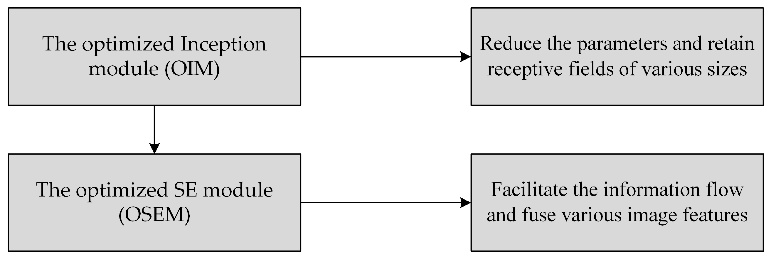
To improve the classification accuracy of TLS_dataset, we propose a novel CNN, namely TL-Net. Inspired by the Inception module and the SE module [11], we propose two novel modules, namely the optimized Inception module (OIM) and the optimized (OSEM). TL-Nets are built by inserting these two new modules into ResNets. The OIM is proposed to reduce parameters and retain receptive fields of various sizes. To further facilitate information flow and fuse various image features, we propose the OSEM based on the SE module (SEM). The results of ablation and comparison experiments verify the effectiveness of these two modules. The method proposed in this paper can retain informative images for transmission line inspection effectively. Hence, our work is of considerable significance in maintaining the reliability and sustainability of transmission networks. The general schematic flowchart of the transmission line scene classification is demonstrated in Figure 2.

2. Related Works

2.1. Machine Learning

Common machine learning algorithms include Support Vector Machine (SVM) [12], Bayesian Additive Regression Tree (BART) [13], and Quantile Regression Forests (QRF) [14]. In recent years, machine learning algorithms have been widely applied in various research domains related to electricity, such as power outage prediction [15], wind speed prediction [16], and storm outage prediction [17]. In [15], Yang et al. proposed a method to quantify the uncertainty in power outage prediction modeling based on machine learning. Cerrai et al. [16] proposed three new modules based on Outage Prediction Model (OPM) and evaluated them on 76 extratropical and 44 convective storms. Bhuiyan et al. [17] evaluated the performance of BART and QRF on wind speed prediction, and their study suggested that QRF outperformed BART.
Due to the working mode of machine learning algorithms, it is necessary to extract image features before training. Common image feature extraction algorithms include Local Binary Pattern (LBP), SIFT (Scale-invariant Feature Transform), and HOG (Histogram of Oriented Gradient) [7]. However, these hand-crafted features cannot simply be adapted to new conditions [1,18]. Hence, the image classification methods, which are based on machine learning, cannot satisfy the accuracy requirements of classification tasks with intricate content, such as transmission line scenes.

2.2. Deep Learning

In 1998, LeCun [19] proposed LeNet to handle the handwritten classification task. However, LeNet suffers from much memory consumption and low efficiency. Hence, this significant innovation drew little attention. In 2012, the success of AlexNet, proposed by Krizhevsky et al., led to the resurgence of CNNs [20]. AlexNet is a significant breakthrough in the field of computer vision due to substantially better accuracy than traditional machine learning methods. Szegedy et al. [21] proposed GoogLeNet, which contains a novel module named the Inception module. The Inception module can merge the feature splits which are produced by various convolution kernels. In 2014, the Visual Geometry Group proposed VGG [22], and the results of their work verify that deeper CNNs usually achieve better accuracy. In contrast to GoogLeNet, VGG stacks 3×3 convolution layers repeatedly to construct the entire network. The strategy of VGG is simple but effective, which is inherited by ResNet. In 2015, He et al. [23] proposed ResNet, and their pioneering work alleviates the notorious problem of vanishing/exploding gradients in deep CNNs, which can obtain high-level semantics of images.
Deep convolutional neural networks have been adopted in different fields, such as insulator detection [24,25] and power line inspection [26,27]. Previous researchers have done lots of work on transmission line scene classification. Yang et al. [28] proposed a method for classifying key images of transmission lines based on Markov Random Fields (MRF). In [29], Kim et al. proposed a method of power line scene classification based on Random Forests (RF). In [30], Zhao et al. proposed a method to classify power line insulator status based on the CNN model with multi-patch feature extraction.

3. Data Collection and Augmentation

3.1. Data Collection

The images in TLS_dataset were captured by cameras during transmission line inspections in China. This original dataset consists of 6000 aerial images, with a resolution of 3×224×224. There are 3000 positive samples and 3000 negative samples in this dataset.

3.2. Data Augmentation

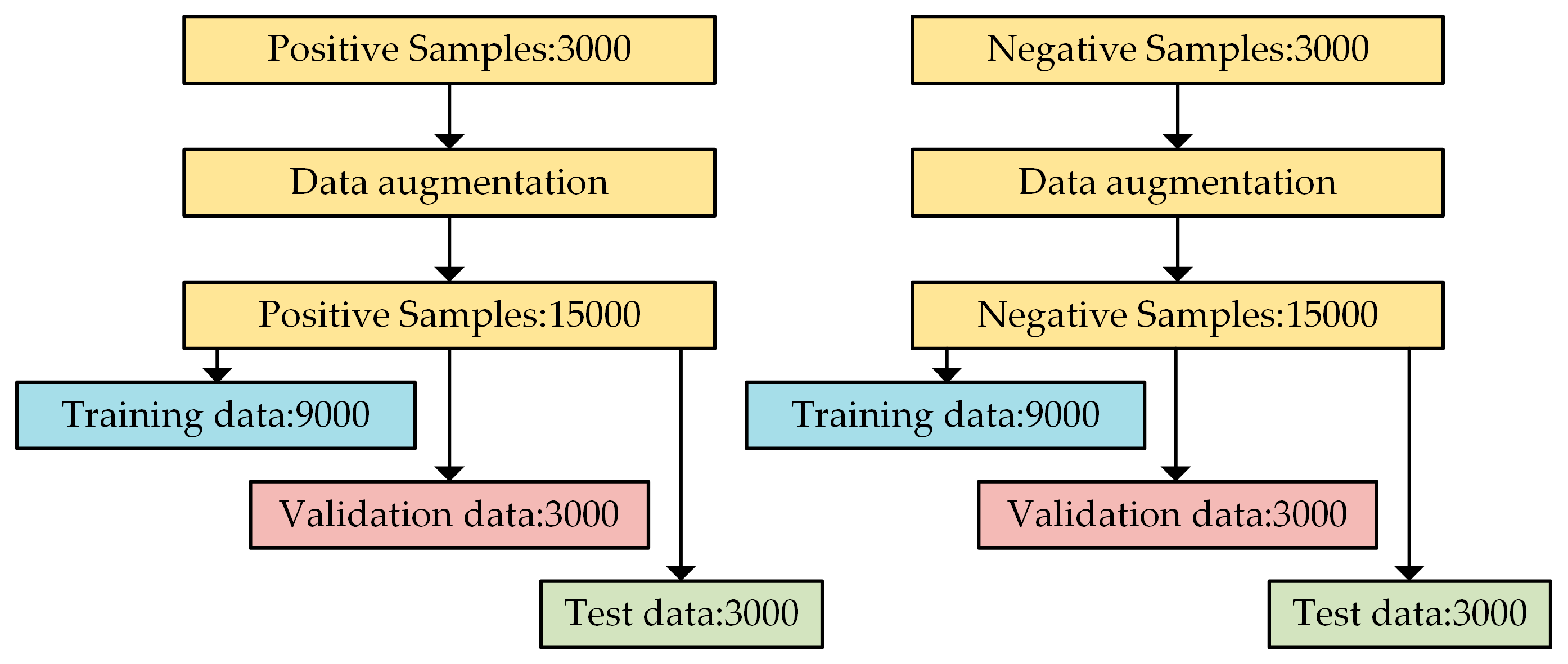
To improve the robustness of classifiers, we improve the number of images with the following methods. After rotating horizontally, rotating vertically, adding noise, and modifying image brightness, the number of images increased fivefold. We set the ratio of training data, validation data, and test data to be 3:1:1, as shown in Figure 3. Specifically, we modify image brightness in the HSV color space and then convert the image format from HSV color space to RGB color space.

4. Method

4.1. Optimized Inception Module

The Inception module is a notable architecture innovation in the development of CNNs, which contains various kernel sizes to extract features of different sizes [21]. Consider a feature map X that is passed through the Inception module. This module implements s transformation functions, denoted by [F1(·), F2(·),···, Fs(·)], which can be regarded as a composite function of various operations, such as convolution, activation function, pooling, and Batch Normalization (BN). The output of the Inception module is denoted by Y, which can be defined as in Equation (1):
Y = C [ F 1 ( X ) , F 2 ( X ) , ... , F s ( X ) ]
where C[·] refers to the concatenation of each feature outputted by different branches. The Inception module can extract features of various receptive fields and merge these features across their channel dimension. However, the Inception module suffers from excessive parameters and a lack of interpretability. Hence, it is unclear how to modify the large numbers of hyper-parameters to adapt to different tasks. To address this challenge, we propose the optimized Inception module (OIM).
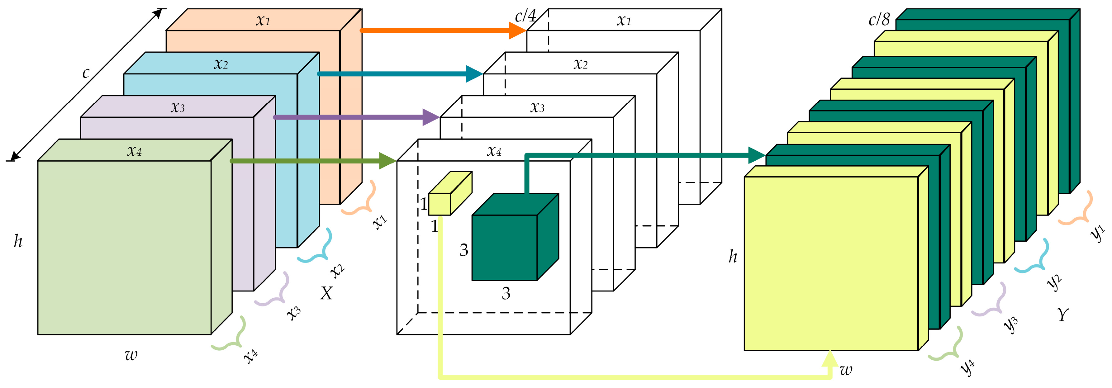
The shortcut connection of ResNets can effectively alleviate the problem of vanishing and exploding gradients in deep networks [23]. Based on the results of previous works, deep networks can extract a large receptive field by small convolution layers [22,23]. Hence, the Inception module, which contains large convolution layers, is not suitable to be inserted into deep networks. In contrast to the Inception module, the OIM comprises 1×1 and 3×3 convolution layers. The 3×3 convolution layer can gain a large receptive field in deep networks, and the 1×1 convolution layer can retain the receptive fields in various sizes. To further reduce the parameters, we insert the grouped convolution into the OIM as depicted in Figure 4.
Consider a feature map X which is passed through the OIM. The input X is split into four parts of the same spatial size. These four feature blocks are denoted by x1~x4. Then, we utilize 1×1 and 3×3 convolution layers to extract multi-scale features of different receptive fields. Then these features are merged across their channel dimension. The concatenation of these features is indicated as yi, where i∈{1,2,3,4}. We refer to the transformation functions of 1×1 and 3×3 convolution layers as Fi(·) and Gi(·). Finally, the output Y is written as in Equation (2):
{ y i = C [ F i ( x i ) , G i ( x i ) ] Y = C [ y 1 , y 2 , y 3 , y 4 ]
where yi refers to the output of the convolution operations. We insert the OIM into ResNets to replace the original 3×3 convolution layers. Consider the input size and the output size of the convolution layer both to be c×h×w. The parameter of the 3×3 convolution layer P3×3 and the parameter of the OIM POIM can be calculated in Equation (3):
{ P 3 × 3 = c × 3 × 3 × c = 9 c 2 P O I M = c 4 × ( 1 × 1 + 3 × 3 ) × c 8 × 4 = 1.25 c 2

4.2. Optimized SE Module

The channel-wise attention strategy can focus on relevant information and filter redundant information to decrease the complexity of image analyses. Momenta presented the SEM in 2017, which is a typical channel-wise attention module [11]. Figure 5 shows the architecture of the SEM, which consists of the squeeze operation and the excitation operation. The feature map X first enters in the squeeze operation, which aggregates X across its spatial dimensions (h×w) and produces the channel descriptor x. The excitation operation follows to capture channel-wise dependencies.
Consider the input X, with a size of c×h×w, that is passed through the SE module. The output Y is given as in Equation (4):
{ x = F s q ( X ) = 1 h × w i = 1 h j = 1 w X ( i , j ) e = F e x ( x ) = f ( g ( x ) ) Y = F s c a l e ( X , e )
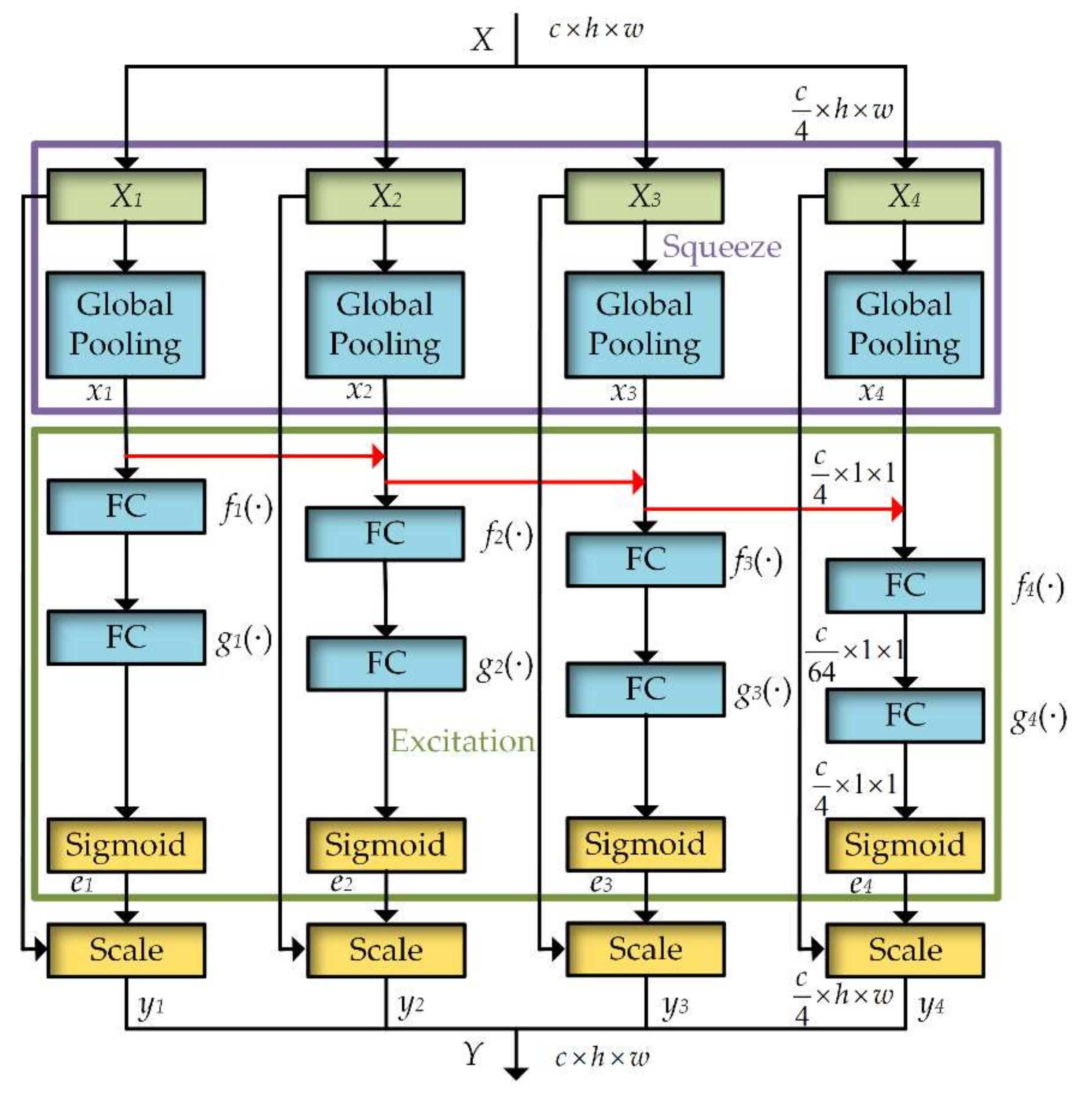
where Fsq(·) and Fex(·) refer to the transformation functions of the squeeze and excitation operations, respectively, and Fscale(X,e) indicates the channel-wise multiplication between X and e. To facilitate information flow further and fuse various channel descriptors, we propose a novel channel-wise attention module based on SEM, which is called OSEM. We split the input X into four parts with the same spatial size, denoted by Xi, where i∈{1,2,3,4}. Each feature block goes through two fully connected layers, which are denoted by fi(·) and gi(·). If a squeeze operation and an excitation operation are implemented on Xi simply, the output Y will lack the dependencies of each feature block. To solve this, we propose a new connectivity pattern: we introduce a direct connection from a channel descriptor xi to the subsequent channel descriptor xi+1. Figure 6 illustrates the architecture of the OSEM. The output Y is written as in Equation (5):
{ x i = F s q ( X i ) = 1 h × w i = 1 h j = 1 w X i ( i , j ) e i = F e x ( j = 1 i x j ) = f i ( g i ( j = 1 i x j ) ) y i = F s c a l e ( X i , e i ) Y = C [ y 1 , y 2 , y 3 , y 4 ]
In the OSEM, each fully connected layer fi(·) and gi(·) could potentially receive channel descriptors from all the preceding feature blocks {xj, ji}. Note that y4 receives channel descriptors of all the feature blocks. This connectivity pattern can enforce the information flow of features and fuse features of different blocks. The information fusion of different feature blocks can make the output of the OSEM contain more image information than that of the SEM. Consider the input size and the output size of the SEM and the OSEM both to be c×h×w. The parameter of the SEM PSEM and the parameter of the OSEM POSEM can be calculated in Equation (6):.
{ P S E M = c 16 × c + c × c 16 = c 2 8 P O S E M = ( c 64 × c 4 + c 4 × c 64 ) × 4 = c 2 32

4.3. Network Implementation Details

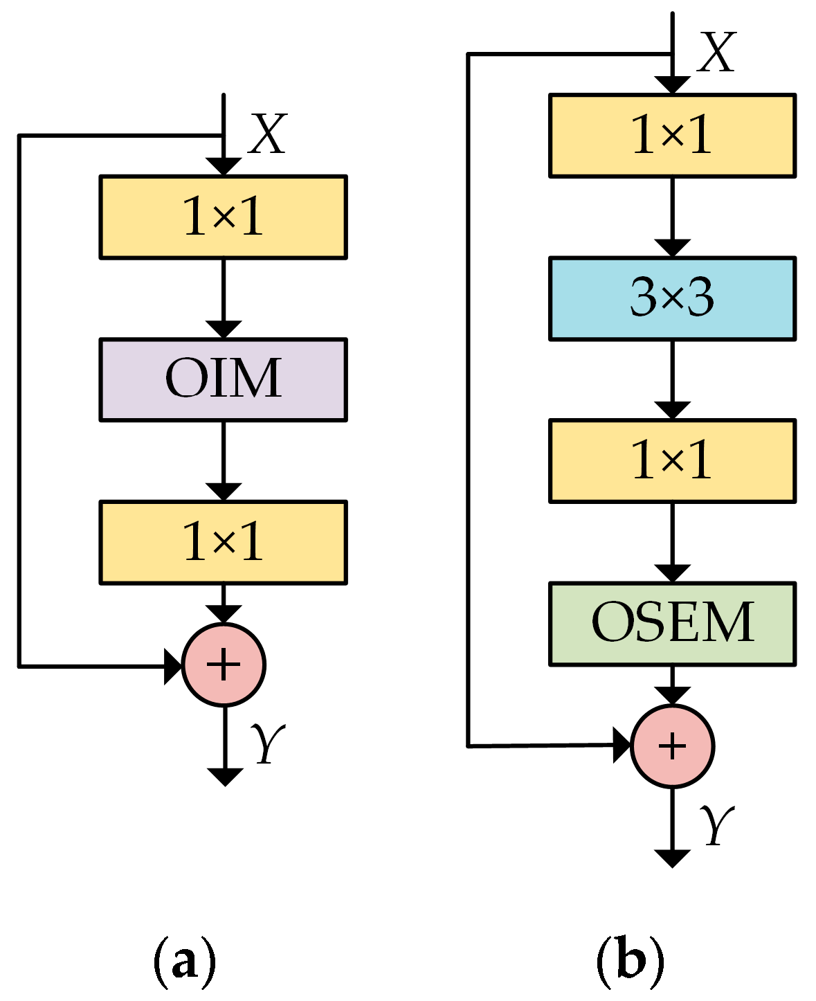
ResNets are composed of basic blocks, as illustrated in Figure 7a. We reformulate the network architecture by inserting the OIM and the OSEM into ResNets. The basic block in TL-Nets is as illustrated in Figure 7b. The implementation of TL-Nets follows [23], as given in Table 1, and we utilize the publicly available framework of Keras to build all the networks in this paper. Consider a 3×224×224 input image that is passed through TL-Nets. Before entering the conv2, a 7×7 convolution operation and a max-pooling are performed on the input image. Downsampling is performed by conv3_1, conv4_1, and conv5_1 with a stride of 2, as suggested in [23]. At the end of TL-Nets, the sigmoid is attached to the average pooling. In this paper, all the networks are trained using SGD (Stochastic Gradient Descent) with a mini-batch size of 10 on a Titan Xp GPU. We set the momentum, the weight decay, and the initial learning rate to 0.9, 10−4, and 0.01, as suggested in [23]. The loss function is set to be binary cross-entropy.

5. Experimental Results and Analysis

5.1. Ablation Studies

To better illustrate the effectiveness of each optimized module, we conduct the ablation study as follows. We evaluate the classification performances of ResNets with each optimized module. To ensure a fair comparison test, we eliminate the differences in hyper-parameter settings. The basic blocks of OI-ResNets and OSE-ResNets are depicted in Figure 8a,b.
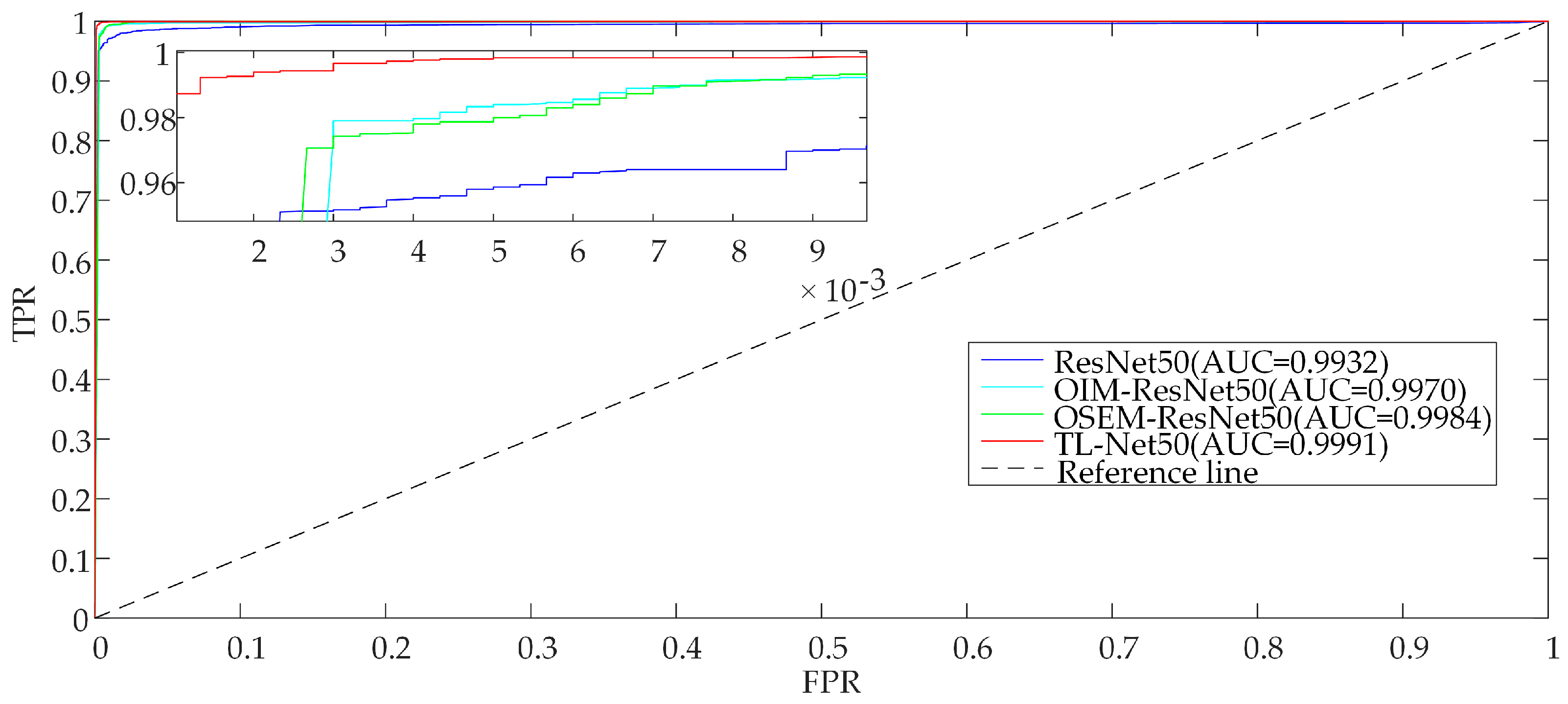
The receiver operating characteristic (ROC) curves are adopted to illustrate the classification performance of binary classifiers with variable thresholds. The area under the ROC curve (AUC) is equal to the probability that the classifier ranks a randomly chosen positive instance higher than a randomly chosen negative one. We evaluate the classification performance of each network by the accuracy of test data and the AUC value, as suggested in [7,31]. The larger the AUC value is, the better the classification performance of the network is. False negative (FN), false positive (FP), true negative (TN), and true positive (TP) are essential parameters in the ROC curve. The true positive rate (TPR) and the false positive rate (FPR) are defined as in Equation (7):
{ T P R = T P T P + F N F P R = F P F P + T N
The accuracy can be calculated in Equation (8):
a c c u r a c y = T P + T N T P + F N + F P + T N
Table 2 shows the accuracies of ResNets with each optimized module. As we can observe, the OIM and the OSEM both improve test accuracy compared to the baseline models. Specifically, OIM-ResNet50 and OSEM-ResNet50 improve test accuracy by 0.84% and 1.09%, respectively, compared to ResNet50. In comparison with ResNet101, OIM-ResNet101 and OSEM-ResNet101 achieve improvements of 1.07% and 1.19% in test accuracy. Moreover, OIM and OSEM can improve the AUC value of ResNets, according to the data in Table 2.
By analyzing the experimental results, it can be concluded that the OIM and OSEM can improve the classification performance of ResNets. Overall, these comparisons explicitly demonstrate that the OIM and the OSEM can improve the classification performance of ResNets effectively. Figure 9 and Figure 10 show the ROC curves of ResNets, OIM-ResNets, OSEM-ResNets, and TL-Nets.

5.2. Comparison with Typical Deep Learning Methods

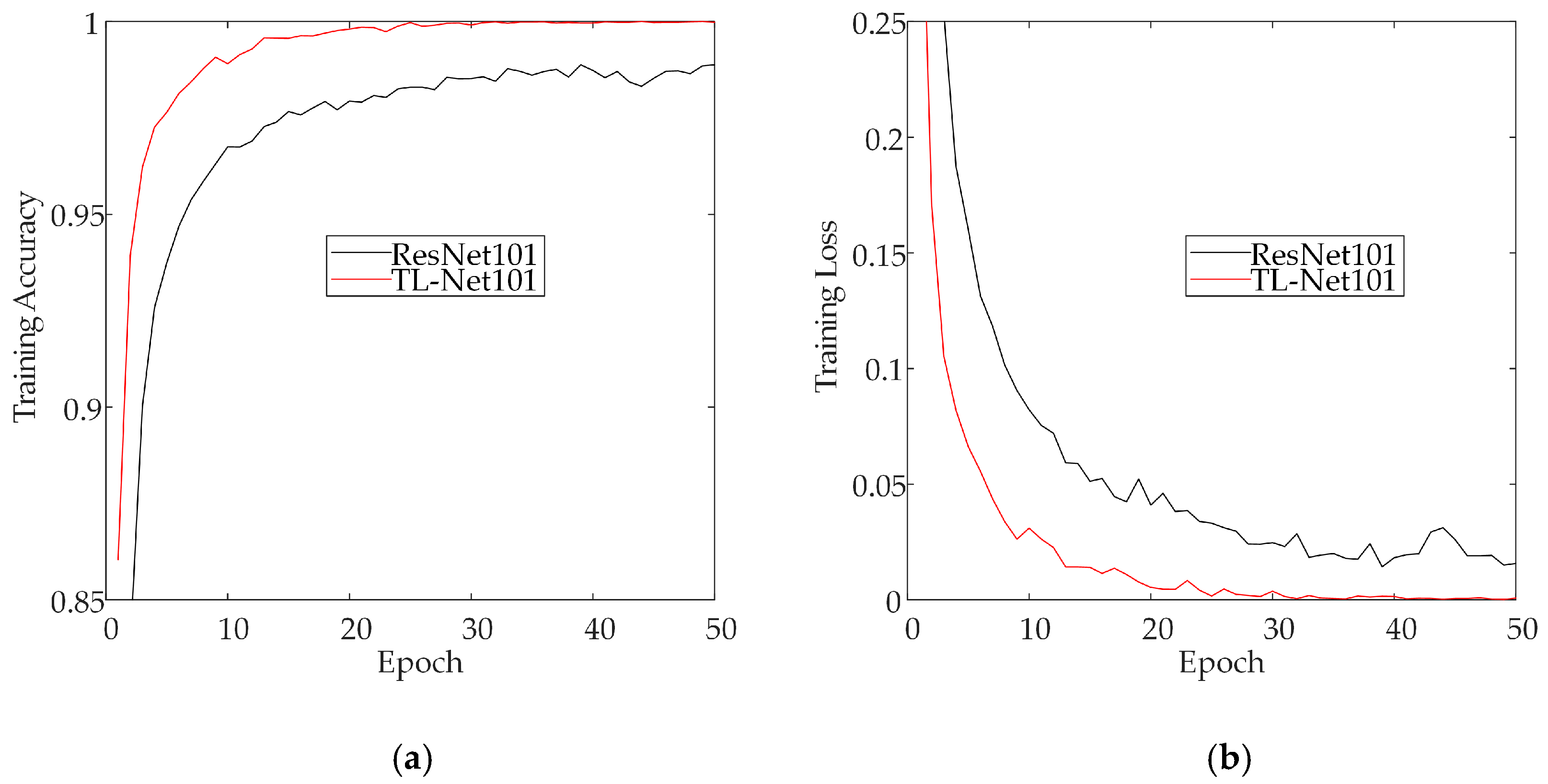
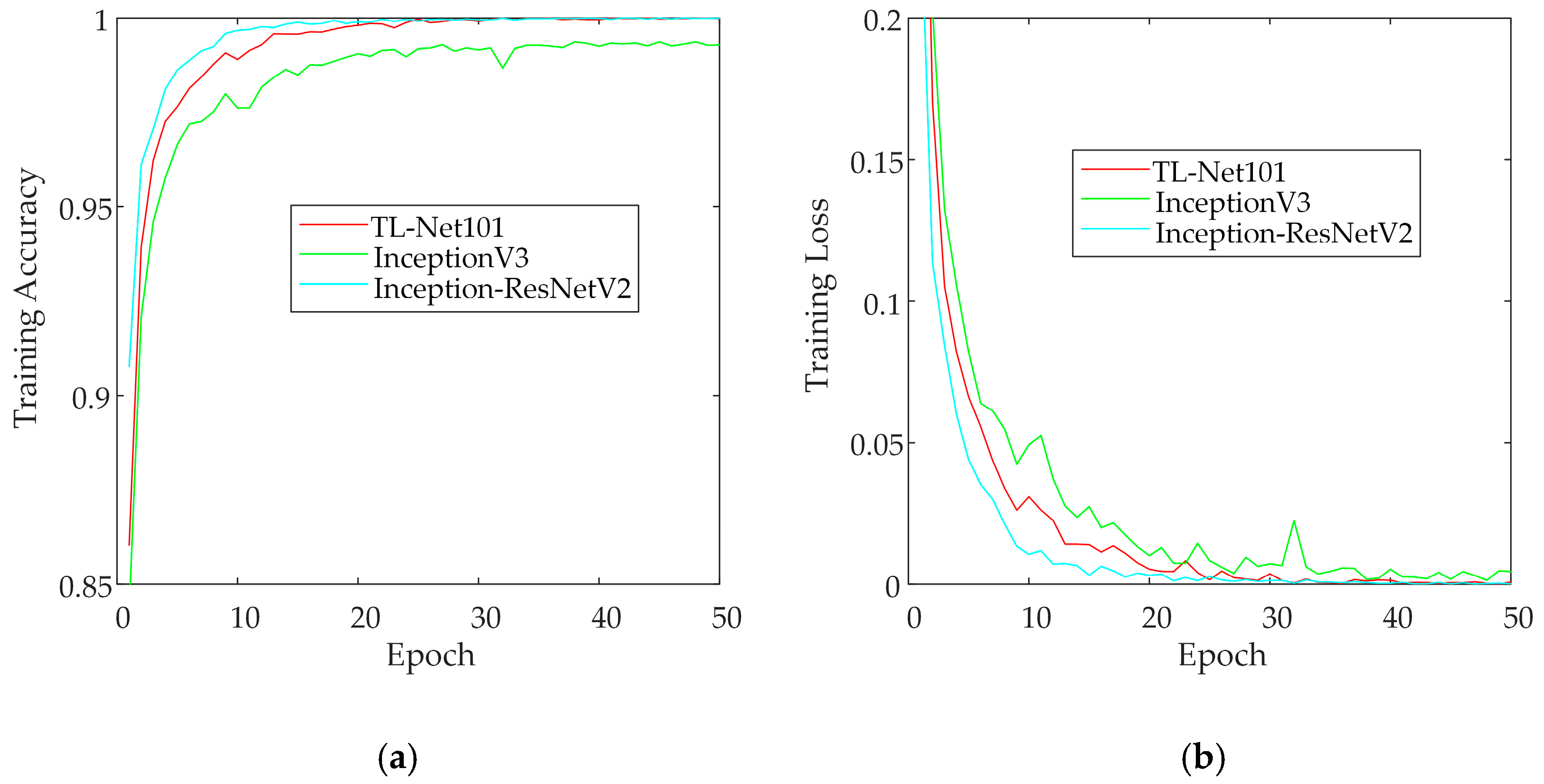
We trained both TL-Nets and some typical CNNs on our test data to validate the effectiveness of TL-Nets. Figure 11 and Figure 12 show the training accuracy curves and training loss curves of ResNets and TL-Nets. Figure 13 shows the training accuracy curves and training loss curves of TL-Net101, InceptionV3 [32], and Inception-ResNetV2 [33]. Table 3 lists the experimental results, which suggest that TL-Net101 achieves the highest test accuracy and AUC value compared to other networks. To be more specific, TL-Net50 and TL-Net101 improve test accuracy by 1.50% and 1.45% compared to baseline models. In comparison to the baseline models, TL-Net50 and TL-Net101 improve the AUC value by 0.0059 and 0.0031. In comparison to InceptionV3 and Inception-ResNetV2, TL-Net101 gains an improvement of 0.81% and 0.10% in test accuracy, respectively. Hence, TL-Nets gain better classification performance than ResNets, which suggests the effectiveness of OIM and OSEM. Figure 14 shows the ROC curves of ResNet50, ResNet101, TL-Net50, TL-Net101, Inception-ResNetV2, and InceptionV3.
Finally, we evaluated the memory consumption and the average running time per image of networks, as shown in Table 4. As we can observe, the average running time of ResNet50 is faster than that of TL-Net50 by 0.006 s. However, the test accuracy of TL-Net50 is higher than that of ResNet50 by 1.50%. We can observe a similar phenomenon in ResNet101 and TL-Net101. Moreover, TL-Net50 gains less memory consumption than ResNets, InceptionV3, and Inception-ResNetV2. Hence, TL-Nets can be seen as a compromise between test accuracy and real-time performance.

6. Conclusions and Future Work

In this paper, we propose a novel network for classifying transmission line scenes, namely TL-Net. TL-Nets are built by inserting two optimized modules into ResNets: the OIM and the OSEM. Specifically, the OIM is designed to reduce network parameters and gain receptive fields of various sizes. The OSEM is proposed to improve information flow and fuse different features. In comparison to other typical deep learning networks, TL-Nets achieve better classification results. Overall, the methods proposed in this paper can improve the accuracy of transmission line scene classification, and they are of considerable significance to the reliability and sustainability of transmission networks.

Author Contributions

Writing, H.L.; methodology, Z.Y. and J.H.; experiments, S.L. and C.Z.; labeling the ground-truth for each image in our dataset, Q.Z. and C.Z.; Q.F. and G.H. provided plenty of aerial images. All authors have read and agreed to the published version of the manuscript.

Funding

This research was supported by the Science and Technology Projects of China Southern Power Grid Co. Ltd. (Grant No. 066600KK52170074), the National Natural Science Foundation of China (Grant No. 61473144), the Fundamental Research Funds for the Central Universities (Grant No. kfjj20190305), the 2019 Science and Technology Project of Jiangxi Provincial Department of Education (Grant No. GJJ191689), and the Natural Science Foundation of Jiangxi Province (Research on Key Technology of Object Detection in Aerial Image of Transmission Line).

Conflicts of Interest

The authors declare no conflicts of interest.

References

  1. Jenssen, R.; Roverso, D. Automatic autonomous vision-based power line inspection: A review of current status and the potential role of deep learning. Int. J. Electr. Power Energy Syst. 2018, 99, 107–120. [Google Scholar] [CrossRef] [Green Version]
  2. Deng, C.; Cheung, H.; Huang, Z.; Tan, Z.; Liu, J. Unmanned aerial vehicles for power line inspection: A cooperative way in platforms and communications. J. Commun. 2014, 9, 687–692. [Google Scholar] [CrossRef] [Green Version]
  3. Akmaz, D.; Mamiş, M.S.; Arkan, M.; Tağluk, M.E. Transmission line fault location using traveling wave frequencies and extreme learning machine. Electr. Power Syst. Res. 2018, 155. [Google Scholar] [CrossRef]
  4. Zhou, Z.; Zhang, C.; Xu, C.; Xiong, F.; Zhang, Y.; Umer, T. Energy-efficient industrial internet of UAVs for power line inspection in smart grid. IEEE Trans. Ind. Inform. 2018, 14, 2705–2714. [Google Scholar] [CrossRef] [Green Version]
  5. Qiu, J. How to build an electric power transmission network considering demand side management and a risk constraint? Int. J. Electr. Power Energy Syst. 2018, 94, 311–320. [Google Scholar] [CrossRef]
  6. Han, J.; Yang, Z.; Zhang, Q.; Chen, C.; Li, H.; Lai, S.; Hu, G.; Xu, C.; Xu, H.; Wang, D.; et al. A method of insulator faults detection in aerial images for high-voltage transmission lines inspection. Appl. Sci. 2019, 9, 2009. [Google Scholar] [CrossRef] [Green Version]
  7. Chan, T.-H.; Jia, K.; Gao, S.; Lu, J.; Zeng, Z.; Ma, Y. PCANet: A simple deep learning baseline for image classification? IEEE Trans. Image Process. 2015, 24, 5017–5032. [Google Scholar] [CrossRef] [Green Version]
  8. Yamato, Y.; Demizu, T.; Noguchi, H.; Kataoka, M. Automatic GPU offloading technology for open IoT environment. IEEE Internet Things J. 2018, 6, 2669–2678. [Google Scholar] [CrossRef]
  9. Pan, B.; Shi, Z.; Xu, X. MugNet: Deep learning for hyperspectral image classification using limited samples. ISPRS J. Photogramm. Remote Sens. 2018, 145, 108–119. [Google Scholar] [CrossRef]
  10. Hinton, G.E.; Osindero, S.; Teh, Y.-W. A fast learning algorithm for deep belief nets. Neural Comput. 2006, 18, 1527–1554. [Google Scholar] [CrossRef]
  11. Hu, J.; Shen, L.; Sun, G. Squeeze-and-excitation networks. In Proceedings of the 2018 IEEE/CVF Conference on Computer Vision and Pattern Recognition, Salt Lake City, UT, USA, 18–22 June 2018; pp. 7132–7141. [Google Scholar]
  12. Foody, G.M.; Mathur, A. The use of small training sets containing mixed pixels for accurate hard image classification: Training on mixed spectral responses for classification by a SVM. Remote Sens. Environ. 2006, 103, 179–189. [Google Scholar] [CrossRef]
  13. Chipman, H.A.; George, E.I.; McCulloch, R.E. BART: Bayesian additive regression trees. Ann. Appl. Stat. 2010, 4, 266–298. [Google Scholar] [CrossRef]
  14. Meinshausen, N. Quantile regression forests. J. Mach. Learn. Res. 2006, 7, 983–999. [Google Scholar]
  15. Yang, F.; Wanik, D.W.; Cerrai, D.; Bhuiyan, A.E.; Anagnostou, E.N. Quantifying uncertainty in machine learning-based power outage prediction model training: A tool for sustainable storm restoration. Sustainability 2020, 12, 1525. [Google Scholar] [CrossRef] [Green Version]
  16. Ehsan, B.M.A.; Begum, F.; Ilham, S.J.; Khan, R.S. Advanced wind speed prediction using convective weather variables through machine learning application. Appl. Comput. Geosci. 2019, 1, 100002. [Google Scholar] [CrossRef]
  17. Cerrai, D.; Wanik, D.W.; Bhuiyan, M.A.E.; Zhang, X.; Yang, J.; Frediani, M.E.; Anagnostou, E.N. Predicting storm outages through new representations of weather and vegetation. IEEE Access 2019, 7, 29639–29654. [Google Scholar] [CrossRef]
  18. Bengio, Y.; Courville, A.; Vincent, P. Representation learning: A review and new perspectives. IEEE Trans. Pattern Anal. Mach. Intell. 2013, 35, 1798–1828. [Google Scholar] [CrossRef]
  19. LeCun, Y.; Bottou, L.; Bengio, Y.; Haffner, P. Gradient-based learning applied to document recognition. Proc. IEEE 1998, 86, 2278–2324. [Google Scholar] [CrossRef] [Green Version]
  20. Krizhevsky, A.; Sutskever, I.; Hinton, G.E. Pdf ImageNet classification with deep convolutional neural networks. Commun. ACM 2017, 60, 84–90. [Google Scholar] [CrossRef]
  21. Simonyan, K.; Zisserman, A. Very deep convolutional networks for large-scale image recognition. arXiv 2014, arXiv:1409.1556. [Google Scholar]
  22. Szegedy, C.; Liu, W.; Jia, Y.; Sermanet, P.; Reed, S.; Anguelov, D.; Erhan, D.; Vanhoucke, V.; Rabinovich, A. Going deeper with convolutions. In Proceedings of the 2015 IEEE Conference on Computer Vision and Pattern Recognition (CVPR), Boston, MA, USA, 7–10 June 2015; pp. 1–9. [Google Scholar]
  23. He, K.; Zhang, X.; Ren, S.; Sun, J. Deep residual learning for image recognition. In Proceedings of the 2016 IEEE Conference on Computer Vision and Pattern Recognition (CVPR), Las Vegas, NV, USA, 27–30 June 2016; pp. 770–778. [Google Scholar]
  24. Zhao, Z.; Zhen, Z.; Zhang, L.; Qi, Y.; Kong, Y.; Zhang, K. Insulator detection method in inspection image based on improved faster R-CNN. Energies 2019, 12, 1204. [Google Scholar] [CrossRef] [Green Version]
  25. Han, J.; Yang, Z.; Xu, H.; Hu, G.; Zhang, C.; Li, H.; Lai, S.; Zeng, H. Search like an eagle: A cascaded model for insulator missing faults detection in aerial images. Energies 2020, 13, 713. [Google Scholar] [CrossRef] [Green Version]
  26. Liu, Y.; Shi, J.; Liu, Z.; Huang, J.; Zhou, T. Two-layer routing for high-voltage powerline inspection by cooperated ground vehicle and drone. Energies 2019, 12, 1385. [Google Scholar] [CrossRef] [Green Version]
  27. Liu, Z.; Wang, H. Automatic detection of transformer components in inspection images based on improved faster R-CNN. Energies 2018, 11, 3496. [Google Scholar] [CrossRef] [Green Version]
  28. Juntao, Y.; Zhizhong, K. Multi-scale features and markov random field model for powerline scene classification. Acta Geod. Cartogr. Sin. 2018, 47, 188. [Google Scholar]
  29. Kim, H.B.; Sohn, G. Point-based classification of power line corridor scene using random forests. Photogramm. Eng. Remote Sens. 2013, 79, 821–833. [Google Scholar] [CrossRef]
  30. Zhao, Z.; Xu, G.; Qi, Y.; Liu, N.; Zhang, T. Multi-patch deep features for power line insulator status classification from aerial images. In Proceedings of the 2016 International Joint Conference on Neural Networks (IJCNN), Vancouver, BC, Canada, 25–29 July 2016; pp. 3187–3194. [Google Scholar]
  31. Wei, D.; Wang, B.; Lin, G.; Liu, D.; Dong, Z.Y.; Liu, H.; Liu, Y. Research on unstructured text data mining and fault classification based on RNN-LSTM with malfunction inspection report. Energies 2017, 10, 406. [Google Scholar] [CrossRef] [Green Version]
  32. Szegedy, C.; Vanhoucke, V.; Ioffe, S.; Shlens, J.; Wojna, Z. Rethinking the inception architecture for computer vision. In Proceedings of the 2016 IEEE Conference on Computer Vision and Pattern Recognition (CVPR), Las Vegas, NV, USA, 27–30 June 2016; pp. 2818–2826. [Google Scholar]
  33. Szegedy, C.; Ioffe, S.; Vanhoucke, V.; Alemi, A.A. Inception-v4, inception-resnet and the impact of residual connections on learning. In Proceedings of the Thirty-first AAAI conference on artificial intelligence, San Francisco, CA, USA, 4–9 February 2017. [Google Scholar]
Figure 1. (a) The positive sample; (b) the negative sample. The positive sample contains critical components of transmission lines, while the negative sample does not.
Energies 13 03910 g001
Figure 2. The general schematic flowchart of the transmission line scene classification.
Energies 13 03910 g002
Figure 3. The method to build the TLS_dataset.
Energies 13 03910 g003
Figure 4. The architecture of the OIM. The input feature map X is split into four parts, denoted by x1~x4. The yellow block denotes the 1×1 convolution layer, and the green one indicates the 3×3 convolution layer. The y1~y4 indicates output feature splits that are merged into Y.
Energies 13 03910 g004
Figure 5. The architecture of the SEM. The purple frame indicates the squeeze operation, and the green frame indicates the excitation operation. FC denotes the fully connected layer. The number of neurons in the first and second fully connected layer is set to c/16 and c, as suggested in [11]. The input is indicated as X, and the output is denoted by Y.
Energies 13 03910 g005
Figure 6. The architecture of the OSEM. The purple frame indicates the squeeze operation, and the green frame indicates the excitation operation. FC denotes the fully connected layer. For each feature block, the number of neurons in the first and second fully connected layer is set to c/64 and c/4. The input is denoted by X, and the output is indicated as Y.
Energies 13 03910 g006
Figure 7. (a) The basic block of ResNets; (b) the basic block of TL-Nets. The input is denoted by X, and the output is indicated as Y.
Energies 13 03910 g007
Figure 8. (a) The basic block of OIM-ResNets; (b) the basic block of OSEM-ResNets. The input is denoted by X, and the output is indicated as Y.
Energies 13 03910 g008
Figure 9. The ROC curves of ResNet50, OIM-ResNet50, OSEM-ResNet50, and TL-Net50.
Energies 13 03910 g009
Figure 10. The ROC curves of ResNet101, OIM-ResNet101, OSEM-ResNet101, and TL-Net101.
Energies 13 03910 g010
Figure 11. (a) The training accuracy curves of ResNet50 and TL-Net50; (b) the training loss curves of ResNet50 and TL-Net50.
Energies 13 03910 g011
Figure 12. (a) The training accuracy curves of ResNet101 and TL-Net101; (b) the training loss curves of ResNet101 and TL-Net101.
Energies 13 03910 g012
Figure 13. (a) The training accuracy curves of TL-Net101, InceptionV3, and Inception-ResNetV2; (b) the training loss curves of TL-Net101, InceptionV3, and Inception-ResNetV2.
Energies 13 03910 g013
Figure 14. The ROC curves of ResNet50, ResNet101, TL-Net50, TL-Net101, Inception-ResNetV2, and InceptionV3.
Energies 13 03910 g014
Table 1. The architecture of TL-Nets for our aerial image dataset. Downsampling is performed by conv3_1, conv4_1, and conv5_1 with a stride of 2.
Layer NameTL-Net50TL-Net101
conv17×7 convolution, 64, stride 2
conv2_x3×3 max pooling, stride 2
[ 1 × 1 ,   64 OIM 1 × 1 ,   256 OSEM ] × 3 [ 1 × 1 ,   64 OIM 1 × 1 ,   256 OSEM ] × 3
conv3_x [ 1 × 1 ,   128 OIM 1 × 1 ,   512 OSEM ] × 4 [ 1 × 1 ,   128 OIM 1 × 1 ,   512 OSEM ] × 4
conv4_x [ 1 × 1 ,   256 OIM 1 × 1 ,   1024 OSEM ] × 6 [ 1 × 1 ,   256 OIM 1 × 1 ,   1024 OSEM ] × 23
conv5_x [ 1 × 1 ,   512 OIM 1 × 1 ,   2048 OSEM ] × 3 [ 1 × 1 ,   512 OIM 1 × 1 ,   2048 OSEM ] × 3
outputAverage pooling, 1-d fc, sigmoid
Table 2. The accuracy of ResNets with each optimized module. “OIM-ResNet” denotes the ResNet with the OIM. “OSEM-ResNet” denotes the ResNet with the OSEM. ”Test_acc” denotes the accuracy on the test data.
ModelTest_accAUC Value
ResNet5098.03%0.9932
OIM-ResNet5098.87%0.9970
OSEM-ResNet5099.12%0.9984
TL-Net5099.53%0.9991
ResNet10198.23%0.9964
OIM-ResNet10199.30%0.9983
OSEM-ResNet10199.42%0.9994
TL-Net10199.68%0.9995
Table 3. The accuracy and AUC of some typical convolutional neural networks (CNNs) and TL-Nets. “Test_acc” denotes the test accuracy.
ModelTest_accAUC Value
InceptionV398.87%0.9974
ResNet5098.03%0.9932
ResNet10198.23%0.9964
Inception-ResNetV299.58%0.9990
TL-Net5099.53%0.9991
TL-Net10199.68%0.9995
Table 4. The memory consumption and the running time of some typical CNNs and TL-Nets. “ART” denotes the average running time per image.
ModelMemory ConsumptionART
InceptionV392 M0.024 s
ResNet5090 M0.017 s
ResNet101163 M0.031 s
Inception-ResNetV2214 M0.050 s
TL-Net5057 M0.023 s
TL-Net101100 M0.048 s