Potential of Thermal Energy Storage for a District Heating System Utilizing Industrial Waste Heat

Abstract

The potential for utilizing industrial waste heat for district heating is enormous. There is, however, often a temporal mismatch between the waste heat availability and the heating demand, and typically fossil-based peak boilers are used to cover the remaining heat demand. This study investigates the potential of applying a thermal energy storage tank at the district heating supply system at Mo Industrial Park in Norway, where waste heat from the off-gas of a ferrosilicon production plant is the main heating source. To cover peak heating demands, boilers based on CO gas, electricity, and oil are applied. The reduction in peak heating costs and emissions is evaluated as a function of tank size for two different scenarios: (1) a scenario where CO gas, which is a byproduct from another nearby industry, is the main peak heating source; and (2) a scenario where no CO gas is available, and electricity is the main peak heating source. The highest economic viability is obtained with the smallest storage tank with a volume of 1000 m${}^3$, yielding a payback period of 7.1/16.2 years and a reduction in total heat production costs of 14.6/10.0% for Scenarios 1/2, respectively. The reduction in CO${}_2$ emissions is 19.4/14.8%, equal to 820/32 ton CO${}_2$ for the analyzed period. Sensitivity analysis shows a significant reduction in payback period for Scenario 2 with increasing electricity prices, while the payback period in Scenario 1 is most sensitive to the emission factors.

1. Introduction

The amount of industrial waste heat available in Europe is estimated to be in the same order of magnitude as the total buildings’ heating demand [1]. Many of these waste heat sources are additionally located in areas with high heat demand density, thus suited to be utilized for district heating (DH). However, a major share of industrial waste heat is currently not utilized. Reasons for this may be both technical and economic barriers for recovering and transporting the heat, as well as geographical and temporal mismatch between the availability of excess heat and the heat demand [2]. Thermal energy storage (TES) is a key technology to overcome this mismatch.

Incorporating TES in DH systems provides a wide range of energetic, economic and environmental benefits through peak shaving, reduction in generation unit size or number of units, increased network management flexibility, etc. [3]. Sensible TES in the form of large hot water accumulation tanks is the most common type of storage in DH systems [4], as this is a well-known and robust technology that has low installation cost, high reliability, short response time, and is relatively easy to install and operate. A TES tank provides short-term storage for covering peak heating demands, thus enabling a larger share of the heating demand to be covered by the DH plant providing base load and reducing the production costs. Moreover, TES combined with electric boilers allow the DH supplier to use electricity for heat production when the prices are low, and at the same time provides added flexibility to the power grid with an increasing share of non-dispatchable renewable energy sources [5,6].

In most cases, TES tanks are applied in DH plants with constant, predictable supply, such as biomass boilers [7] or combined heat and power (CHP) plants [8]. In such applications, using TES allows for more optimal sizing and operation of DH plants, enabling the plant to run a larger share of time at full capacity [7]. In terms of industrial waste-heat utilization for DH, as the most excess heat is often available in the summertime, the use of seasonal TES systems is often suggested [9,10]. In Sweden, a seasonal storage system based on borehole TES has also been implemented [11]. There are, however, few studies on evaluating the potential of using TES tanks to reduce the use of peak heating boilers caused by variations in waste heat availability on shorter time scales.

At Mo Industrial Park in Mo i Rana, Norway, waste heat from the off-gases of a ferrosilicon production plant is utilized for supplying heat to the city of Mo i Rana. The total annual amount of available waste heat exceeds the DH demand in Mo i Rana by far; however, peak heating boilers based on CO gas, electricity, and oil are needed during peak demand periods owing to rapid fluctuations in the waste heat availability and the heating demand. Even if the use of peak heating sources is generally low, it constitutes a significant share of the total costs and emissions for the heat production.

This study investigates the potential of applying a TES tank to reduce the costs and emissions related to peak heating at the DH production system at Mo Industrial Park. Using data for DH production and demand, the potential reduction in peak heating as a function of TES tank size is first investigated with a steady-state algorithm. The reduction in peak heating costs and emissions is consequently calculated for the different tank sizes. Two different scenarios have been analyzed: (1) a scenario where CO gas, which is a byproduct from another nearby plant in the industry park, is the main peak heating source; and (2) a scenario where no CO gas is available, and electricity is the main peak heating source. Scenario 1 represents the current operation strategy; however, the availability of CO gas is to some degree uncertain and limited due to variation in production and other users of the gas in the park, rendering Scenario 2 interesting for the study.

2. Materials and Methods

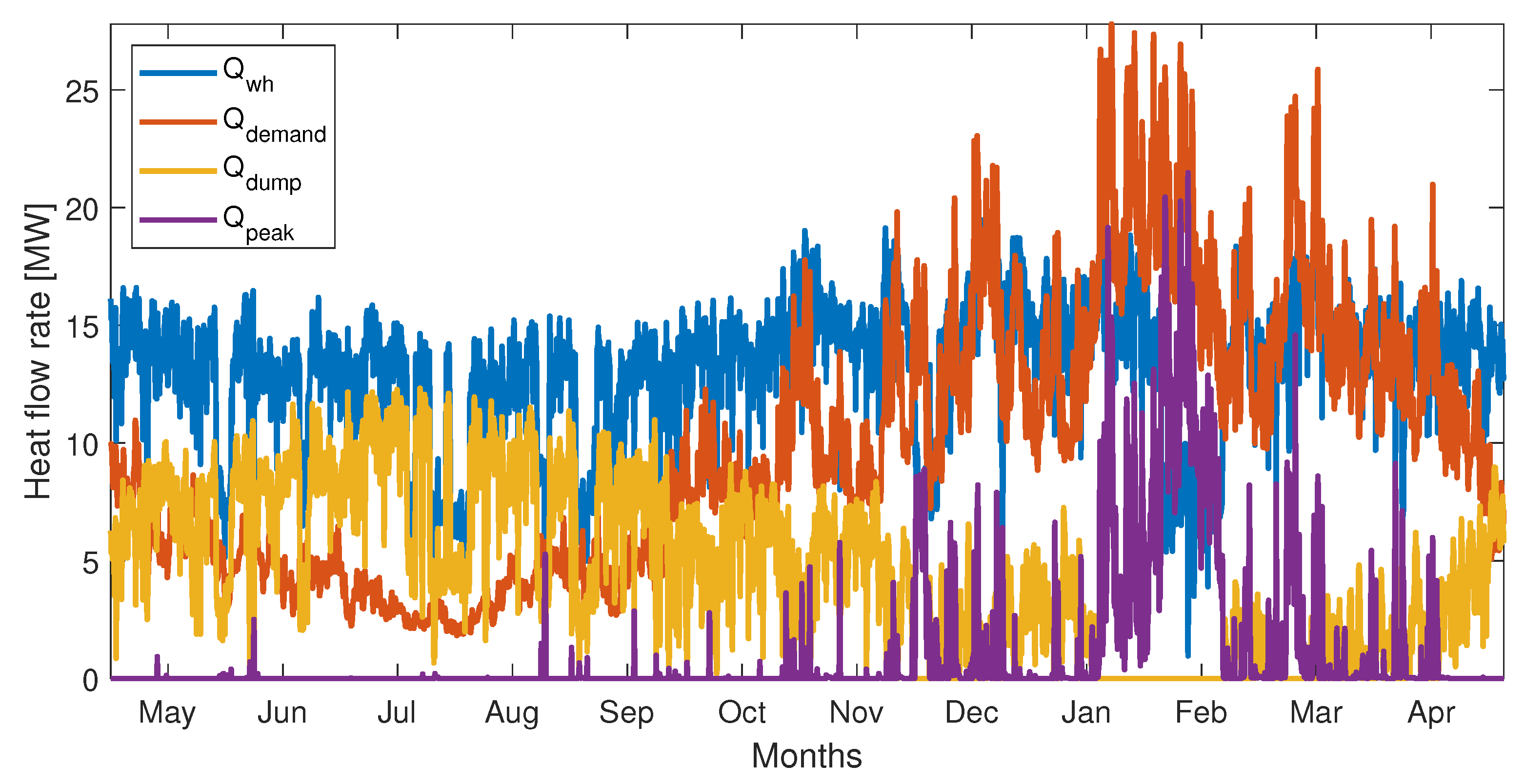
2.1. Case Study Description

Figure 1 presents the DH supply system at Mo Industrial Park. The main heat sources in the system are boilers 5 and 6, which exchange heat with the off-gas through a steam cycle. The steam temperature is typically 125–130 ${}^{\circ }$C (1.9 bar), and the maximum temperature limit out of boiler 5 and 6 is currently 115 ${}^{\circ }$C; however, this limit may be increased to 120 ${}^{\circ }$C if a TES tank is implemented. The DH supply temperature is outdoor compensated between 90 and 105 ${}^{\circ }$C at ambient temperatures ranging from +5 (or higher) to −20 ${}^{\circ }$C (or lower). The return temperature is typically 55 ${}^{\circ }$C, but varies between 50 and 70 ${}^{\circ }$C, depending on the season.

If the water temperature obtained from boilers 5 and 6 drops below the desired supply temperature level, peak heating boilers (1–4) are used. All the boilers are equipped with energy meters, and the DH demand in the network is thus calculated as

$$Q_{demand}=Q_{wh2dh}+Q_{peak}$$

(1)

where $Q_{wh2dh}$ is the waste heat delivered to the DH network from boilers 5 and 6, and $Q_{peak}$ is the total peak heating supply from boilers 1–4.

Table 1. The capacities, energy sources, and prioritization of the different boilers in the two evaluated scenarios (NA = Not available).

Boiler	Energy Source	Capacity	Priority
			Scenario 1	Scenario 2
1	Oil	10 MW	NA	3
2	CO	10 MW	2	NA
3	Oil	10 MW	NA	NA
4	Electricity	13 MW	3	2
5	Off-gas	8 MW	1	1
6	Off-gas	8 MW	1	1

lists the capacities and energy sources for the different boilers shown in Figure 1. Boiler 2 runs on CO gas, which is a by-product from the industry park, and thus normally the prioritized peak heating source. The availability of CO gas is, however, to some degree uncertain due to varying operating conditions of the plant with CO gas as byproduct, and limited due to other users of the gas in the industry park. Therefore, two different scenarios were analyzed:

• CO gas available: CO (boiler 2) as the primary and electricity (boiler 4) as the secondary peak heating source.
• CO gas not available: Electricity (boiler 4) as the primary and oil (boiler 1) as the secondary peak heating source.

The prioritization of the different boilers in these two scenarios is shown in Table 1. Boiler 3 is a reserve boiler that is normally not in use and was therefore omitted from the analysis.

Boilers 5 and 6 dump heat whenever the DH demand is lower than the required cooling of the off-gas from the ferrosilicon furnaces. Figure 2 shows data for hourly average waste heat available (including the waste heat delivered to the DH network and the heat that is dumped), DH demand, peak heating as well as excess heat that is dumped for the analyzed period, May 2018–April 2019. The start of 2018 was omitted from the analysis due to a maintenance stop at boiler 6 and low off-gas temperatures during this period. The total demand, peak heating, and excess heat for the period were 85.2 GWh, 9.2 GWh, and 39.0 GWh, respectively. Although most excess heat is available in the summer, substantial amounts of heat are dumped also during winter, in periods when the waste heat availability suddenly becomes higher than the demand.

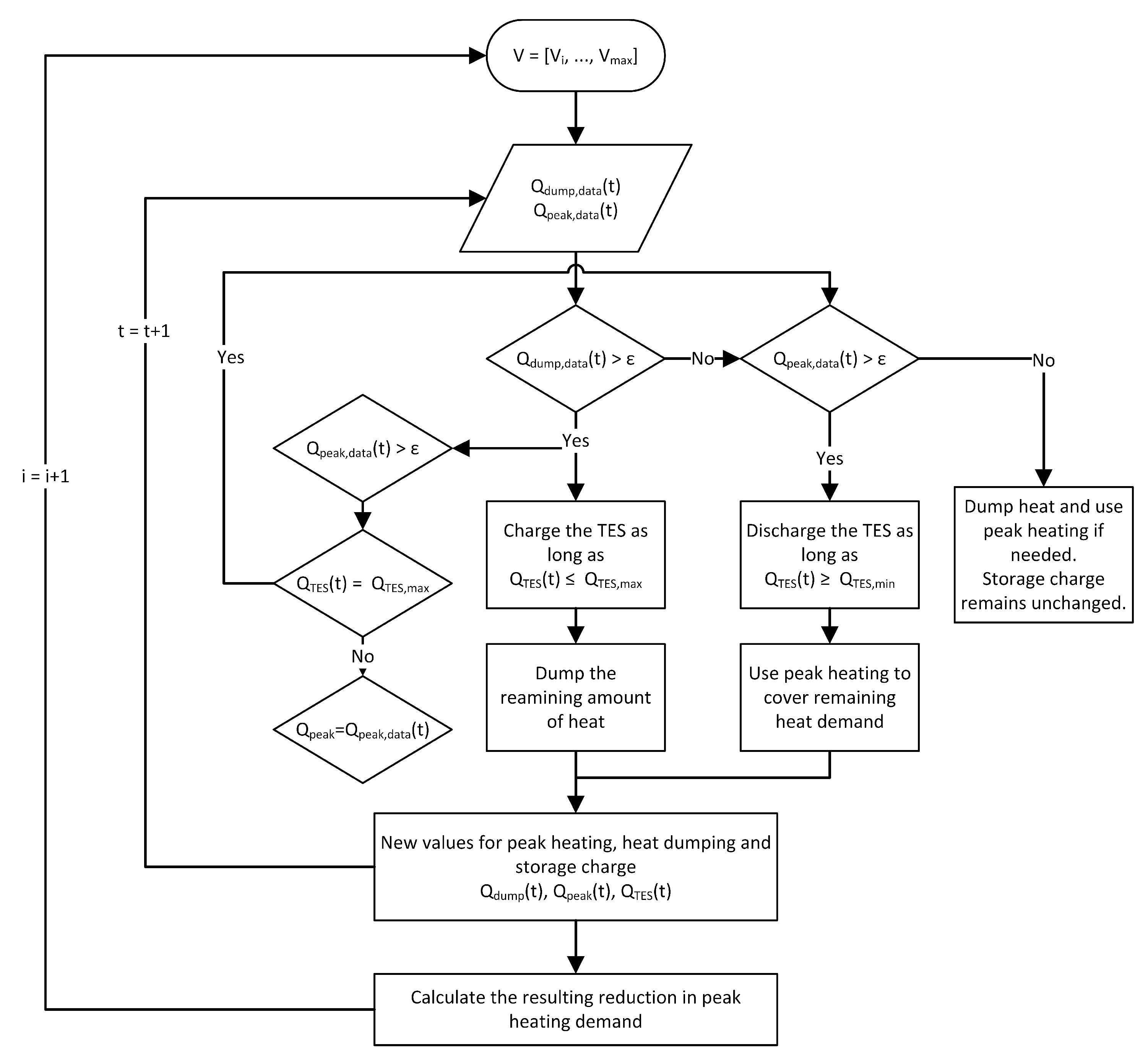
2.2. Calculating the Reduction in Peak Heating as a Function of Tank Size

In the case of a constant, predictable source, the TES tank is usually dimensioned from the basis of load data, see, e.g., [7,12,13]. In the present case, with varying availability of heat, the peak reduction potential of a tank with certain size was calculated using hourly average data for heat flow rates for peak heating and heat dumping using an iterative approach, inspired by [14]. A flow chart of the approach, implemented in MATLAB, is shown in Figure 3. The tank volume was varied from 1000 to 5000 m${}^3$ in steps of 1000 m${}^3$, and the storage capacity for each tank size $V_i$ was calculated as

$$Q_{TES,max,i}=V_i\rho c_p(T_{max}-T_{min}),$$

(2)

where $\rho$ is the density and $c_p$ is the specific heat capacity of water. $T_{max}$ and $T_{min}$ are the maximum and minimum tank temperatures, set to 120 ${}^{\circ }$C and 55 ${}^{\circ }$C, respectively, corresponding to the potential maximum temperature out of boilers 5 and 6, and the average return temperature from the DH network. The temperature level of the tank was not considered, i.e., the analysis was entirely based on energy balances. The tank is charged when there is excess heat available until the tank is full ($Q_{TES}\le Q_{TES,max}$), corresponding to a situation where the maximum temperature level is reached in the entire tank. The tank is discharged when there is a demand for peak heating, provided that there is heat left in the tank ($Q_{TES}>0$), i.e., until the entire tank is at the minimum temperature level. As shown in Figure 3, the tank is charged/discharged only if the data for heat dumping/peak heating rate is above a threshold value $ϵ$ set equal to 1 kW. Values below this were regarded as noise in the measurement data and not as available heat. The calculation was carried out at an hourly basis, from the start of May 2018 until the end of April 2019.

The hourly heat losses from the tank were set to a constant value of 0.03%. This value was calculated from the basis of the surface area and storage capacity for the smallest tank (1000 m${}^3$), and an assumed maximum temperature difference between the tank and the ambient (140 K, corresponding to an outdoor temperature of −20 ${}^{\circ }$C). The tank insulation was assumed to have a thermal conductivity of 0.05 W/(m$·$K) and a thickness of 300 mm. The storing efficiency of the tank, equal to 1 − heat losses, is thus very high (99.97%). The charging and discharging efficiency of a TES tank is related to the pumping efficiency, which only affects the electricity consumption. The study focuses on thermal energy and the charging and discharging efficiencies were thus not considered in the model.

2.3. Economic Evaluation

Having determined the total reduction in peak heating for different tank sizes, the heat production was allocated to the different peak heating boilers using the available data. The obtained reduction in peak heating was applied to first cut peak heating from boiler 1 (oil), thereafter boiler 4 (electricity), and finally from boiler 2 (CO), see Table 1. In Scenario 1, no oil is available, and any remaining peak heating demand on boiler 1 was allocated to boiler 4. In Scenario 2, no CO is available, and all remaining peak heating demand on boiler 2 was thus allocated to boiler 4.

The reduction in peak heating costs was thereafter calculated based on heat production costs for different peak heating sources, obtained from the DH supplier (Mo Fjernvarme AS). For CO and oil, constant price per kWh was applied. For electricity, the grid tariff depends on the total annual power demand, with a stepwise reduction in the tariff with an increase in demand by 1000 MWh. For the electricity price, different scenarios were evaluated. The energy prices are confidential and thus not shown. The payback period of a TES tank with a given size, $N_{0,i}$, was calculated according to

$$N_{0,i}=\frac{ln\left(B_i/(B_i-I\left(V_i\right)·r)\right)}{ln(1+r)},$$

(3)

where $B_i$ is the savings in the form of reduction in peak heating costs and emissions taxes, $I\left(V_i\right)$ is the investment cost for a tank with a given size, and r is the interest rate. The interest rate was set to 8%, a value normally used by the DH supplier in their investment analysis. Data for investment costs for TES tanks of different sizes (confidential) were obtained from a Nordic supplier [15]. The costs were given in euros, and an exchange rate of 10 NOK/€ was applied for conversion. The investment costs apply for a pressurized TES tank allowing temperatures up to the maximum temperature of 120 ${}^{\circ }$C, and include insulation, safety apparatus, and internal diffusers. Based on a dialogue with the supplier, an addition of +30% was included in the costs to account for groundwork and additional infrastructure.

Emissions

The CO${}_2$ and NO${}_x$ emissions resulting from peak heating were calculated using yearly emission factors for the different sources given in

Table 2. Emission factors for CO${}_2$ and NO${}_x$ per kWh produced heat.

	CO${}_2$ Emissions [kg/kWh]	NO${}_{\mathit{x}}$ Emissions [kg/kWh]
CO	0/0.574	0.55$·{10}^{-3}$
Electricity	0	0
Oil	0.289	0.211$·{10}^{-3}$

, based on [16,17]. The CO${}_2$ emission factor for electricity was set to 0 as the electricity used is 100% renewable, with guarantees of origin. For CO gas, the DH supplier has until now been granted free quotas for CO${}_2$; however, this may change in near future. Two alternative CO${}_2$ emission factors were thus evaluated for CO, 0 and 0.574 kg/kWh, as shown in Table 2. The DH supplier pays taxes based on the resulting emissions, currently equal to 250 NOK per ton CO${}_2$, and 10,500 NOK per ton NO${}_x$. The CO${}_2$ tax is, however, expected to vary significantly in the years to come, and a sensitivity analysis was therefore carried out, varying the present tax by ±50%. For oil, 25% of the CO${}_2$ tax is already included in the purchase price of the energy, and this was also taken into account in the analysis.

3. Results and Discussion

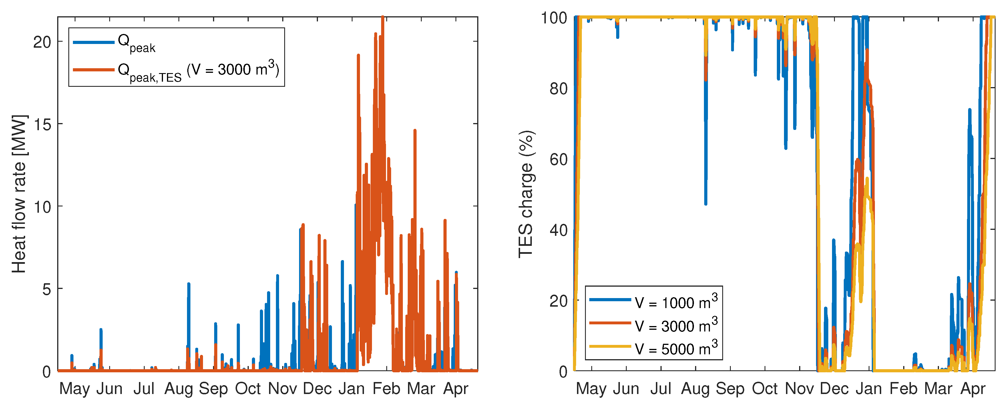
3.1. Reduction in Peak Heating

Figure 4 (left) shows the hourly peak heating for the evaluated period based on data, and the required peak heating when using a TES tank with a volume of 3000 m${}^3$. During the autumn, from August to December, the tank reduces the peak-heating demands significantly; on the contrary, in the period from January to February, there is not enough excess heat to charge the TES tank and the demand for peak heating is nearly as high as without a tank.

Figure 4 (right) shows the hourly relative TES charge (%) for three selected tank sizes for the evaluated period. Covering a peak heating demand, e.g., the prominent peak occurring in August, will reduce the relative charge of a smaller tank more than the relative charge of a larger tank. At the same time, when there is excess heat available, a smaller tank will reach its maximum level faster, as is seen e.g., for the period occurring at the end of December/start of January.

In the summer months from May to July, there are a few occasions when heat was dumped and peak heating was needed at the same time (see Figure 2). In such occasions, discharging of the TES tank is allowed if it is fully charged; otherwise, peak heating is used as shown in the flowchart in Figure 3. The tank cannot be charged and discharged at the same time; charging of the tank was thus prioritized as long as the tank was not full. Simultaneous dumping and peak heating may be related to short-time shut-down of the ferrosilicon production plant, followed by a rapid ramp-up, which results in an overshoot in the waste heat delivery and thus a demand for heat dumping. Such occasions are nevertheless rare and have a negligible impact on the total peak heating demand. Indeed, the peak heating demand in the period May–July 2018 constitutes only 1.9% of the total heating demand for the analyzed period.

Figure 5 shows the total annual peak heating per source for the two different scenarios as a function of tank size. In Scenario 1, applying a TES tank with a small volume has little effect on the electricity use, as the remaining peak heating with oil is allocated to electricity, as explained in Section 2.3. With increasing tank size, however, a clear reduction in both CO and electricity use is visible, with a reduction of up to 11% in electricity and 24% in CO use with a 5000 m${}^3$ tank. In Scenario 2, the share of peak heating covered by oil is small and thus also the reduction in oil use is less visible than reduction in electricity use. Nevertheless, the reduction with a 5000 m${}^3$ tank is 20% for oil and 23% for electricity.

3.2. Reduction in Emissions

Figure 6 shows the reduction in CO${}_2$ and NO${}_x$ emissions as a function of tank size for both the scenarios. For CO${}_2$ emissions in Scenario 1, both the present situation with an emission factor of 0 for CO and a future scenario with an emission factor of 0.574 kg/kWh are shown (see Table 2). With zero emission factor for CO, the emissions result solely from the use of oil, and are on the same level as in Scenario 2 when no TES is used. With introduction of a TES tank, the emissions are reduced to 0 in Scenario 1 as the use of oil is allocated to electricity (see Section 2.3). For Scenario 2, introducing a TES tank has generally a negligible effect on the emissions, as the electricity used by the DH supplier is 100% renewable, and the share of oil in peak heating is minimal.

3.3. Economic Evaluation

Figure 7 shows the relative reduction in peak heating costs, considering energy costs alone. The initial peak heating costs are slightly higher in Scenario 1; thus, the reduction in costs resulting from the implementation of a TES tank is also higher. The reduction in costs is in both scenarios clearly highest for the first step from no TES to implementing a tank with a volume of 1000 m${}^3$. For Scenario 2, the costs increase with tank sizes larger than 2000 m${}^3$, which results from the applied stepwise increase in electricity price as explained in Section 2.3: with a 2000 m${}^3$ tank, the annual electricity demand is slightly above 7000 MWh, while, with a 3000 m${}^3$ tank, the annual electricity demand drops to just below 7000 MWh, resulting in an increase in electricity price and consequently higher energy costs. When the tank size is increased further, the electricity demand continues to decrease while the price stays at the same level, resulting in a decrease in the relative energy costs again.

Table 3. Payback period, and the relative reduction in total peak heating costs and CO${}_2$/NO${}_x$ emissions for all scenarios and tank sizes.

	Scenario 1					Scenario 2
Volume (m${}^3$)	1000	2000	3000	4000	5000	1000	2000	3000	4000	5000
Payback period (years)	7.1	14.2	24.3	–	–	16.2	–	–	–	–
Reduction in total costs (%)	14.6	18.5	20.2	21.7	23.0	10.0	13.7	10.0	11.8	13.6
Reduction in CO${}_2$ emissions (%)	19.4	22.1	23.9	25.6	27.9	14.8	16.3	18.5	19.8	19.8
Reduction in NO${}_x$ emissions (%)	18.4	21.0	22.9	24.6	26.9	14.8	16.3	18.5	19.8	19.8

shows the payback period for TES tanks of different sizes, together with the relative reduction in total operating costs and CO${}_2$ emissions for the analyzed period. In these results, for CO gas, the future scenario of nonzero CO${}_2$ emission factor was assumed for Scenario 1. For Scenario 2, the savings are smaller than the investment times the discount rate for tank sizes larger than 1000 m${}^3$; i.e., $B_i-I\left(V_i\right)·r<0$ in Equation (3). For Scenario 1, this applies for tank sizes larger than 3000 m${}^3$.

According to Rathgeber et al. [18], for the industry, high interest rates (≥10%) and short payback periods of five years and below are usual, while, for the buildings sector, interest rates of 5% and payback periods of 15–20 years are common. A DH system, with an interest rate of 8% as defined by the supplier, lies somewhere in between. A payback period of 7–10 years, obtained for the smallest tank size in Scenario 1, is thus deemed acceptable, and this is also the feedback obtained from the DH supplier. The study by Rathgeber et al. additionally concludes that the viability of a TES for a given application is largely dependent on the number of storage cycles per year [18]. A short-term TES as evaluated here, with several hundred cycles per year, allows much higher costs per installed storage capacity than a seasonal TES because of the larger energy turnover.

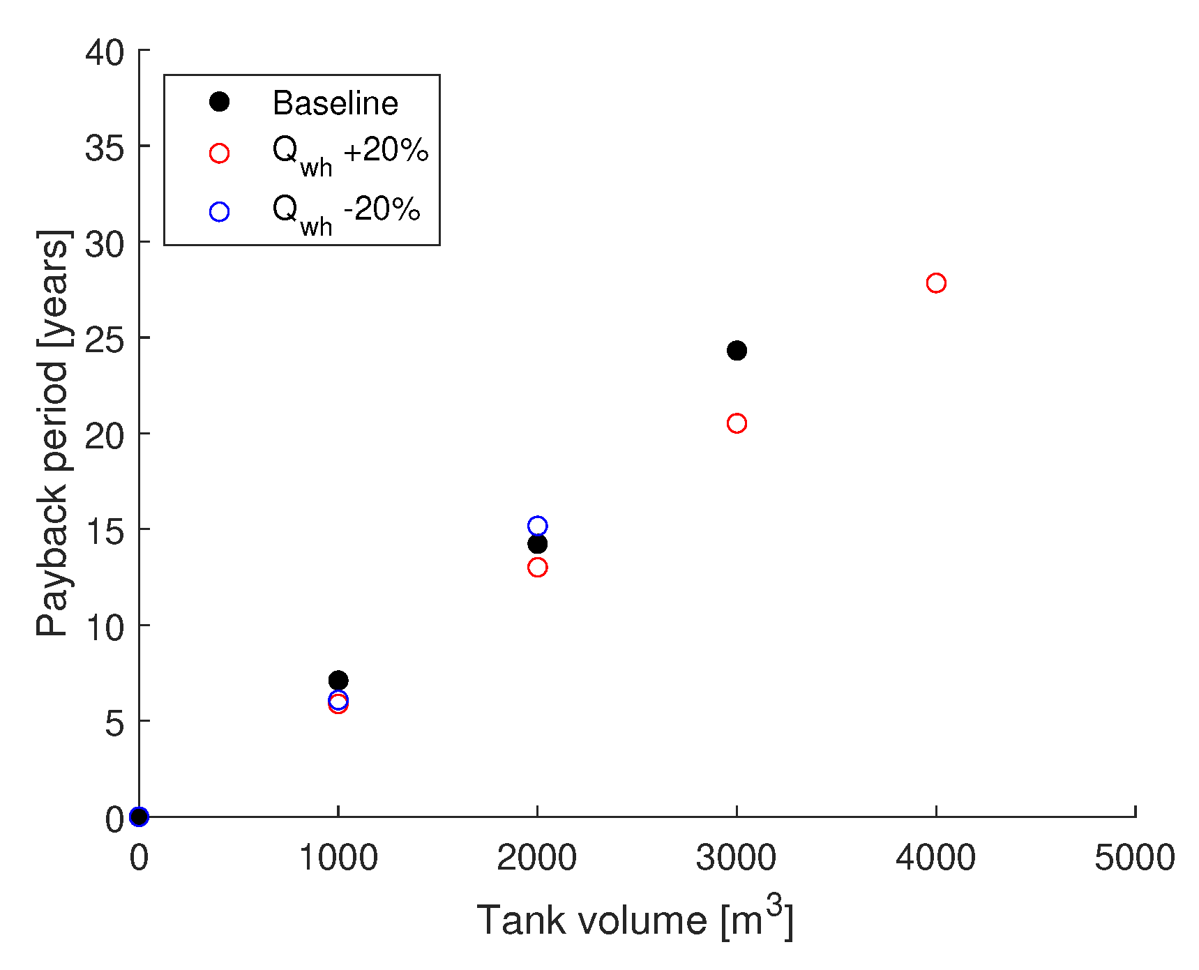
3.4. Sensitivity Analysis

There are several parameters for costs in energy and emissions that affect the payback period significantly. In addition, the analysis was carried out using data for one year, and in reality both the heat demand and the availability of waste heat will vary from year to year. A sensitivity analysis was therefore carried out, considering variation in the following parameters:

• CO emission factor: 0/0.574 kg/kWh, where 0.574 kg/kWh is considered as the baseline
• CO${}_2$ tax: ±50% variation from the baseline of 250 NOK/ton
• Electricity prices: ±43% variation
• Interest rate: varied from 4 to 12% with 8% as the baseline
• Waste heat: ±20% variation in the amount of available waste heat

These ranges were selected based on recommendations from the DH supplier.

Figure 8 presents the results from the sensitivity analysis with respect to the economic parameters. For both scenarios, the payback period is strongly affected by the interest rate. For scenario 2, the investment is not economically viable (i.e., $B_i-I\left(V_i\right)·r<0$) for tank sizes larger than 1000 m${}^3$, unless the interest rate is reduced by 50%; and, for scenario 1, this applies for tank sizes larger than 3000 m${}^3$.

Apart from the interest rate, the payback period for Scenario 1 is most sensitive to the emission factor for CO, and thereafter to the CO${}_2$ tax. The payback period is nevertheless little affected by these parameters at the smallest tank size of 1000 m${}^3$, which appears to be the overall best option based on the results in Figure 5, Figure 6, Figure 7 and Figure 8 and Table 3. For Scenario 2, the payback period is very sensitive to the electricity prices, and hardly affected by the remaining two parameters.

Figure 9 shows the variation in payback period with variation in available waste heat for Scenario 1. For the smallest tank size, the payback period is reduced both with increase and decrease in the amount of waste heat available. This is related to the fact that, in Scenario 1, any remaining peak heating with oil is allocated to electricity when a TES tank is introduced as mentioned earlier. This results in a reduction in the total peak heating costs owing to lower costs for electricity compared to oil, even with less reduction in total peak heating. At larger tank sizes, a decrease in waste heat availability increases the payback period as expected, rendering the investment infeasible at tank sizes larger than 2000 m${}^3$. An increase in waste heat availability on the other hand decreases the payback period significantly, in particular at larger tank sizes.

For Scenario 2, an increase in waste heat availability reduces the payback period at the smallest tank size from 16.2 to 12.0 years, while for larger tank sizes the investment is not economically viable. A decrease in the availability renders the investment nonviable already at the smallest tank size.

Overall, the sensitivity analysis shows that, at larger tank sizes (>2000 m${}^3$ for Scenario 1, >1000 m${}^3$ for Scenario 2), the uncertainty becomes so high that the results can hardly be used as a reliable basis for investment decisions. This is particularly the case for Scenario 2. This also strengthens the conclusion that the smallest tank size of 1000 m${}^3$ is the best option for the present study.

4. Conclusions

This study demonstrates the potential of a TES tank in reducing the costs and emissions related to peak heating at a DH production system based on the utilization of rapidly varying industrial waste heat source. The highest economic viability is obtained with the smallest storage tank with a volume of 1000 m${}^3$, yielding a payback period of 7.1/16.2 years and a reduction in total costs of 14.6/10.0% for Scenarios 1/2, respectively. The reduction in CO${}_2$ emissions is 19.4/14.8%, which is equal to 820/32 ton CO${}_2$ for the analyzed period.

The profitability of implementing a TES tank thus depends strongly on the heat production scheme. In Scenario 1, more expensive and polluting peak heating sources are used, rendering the implementation of a TES tank more profitable. The results are, however, highly sensitive to the energy prices, the applied values for emission taxes, the interest rate, as well as the waste heat availability. Sensitivity analysis showed a significant reduction in the payback period for Scenario 2 with an increase in electricity prices, while the payback period in Scenario 1 is most sensitive to the emission factors. Overall, the sensitivity analysis showed an increasing uncertainty in the payback period with increasing tank size.

The results of the study are used as a basis for an investment decision at the DH supplier. In a further phase of the study, dynamic simulations are applied to evaluate optimal control strategies for the TES tank.

References

1. Persson, U.; Möller, B.; Werner, S. Heat Roadmap Europe: Identifying strategic heat synergy regions. Energy Policy 2014, 74, 663–681. [Google Scholar] [CrossRef]
2. Miró, L.; Gasia, J.; Cabeza, L.F. Thermal energy storage (TES) for industrial waste heat (IWH) recovery: A review. Appl. Energy 2016, 179, 284–301. [Google Scholar] [CrossRef] [Green Version]
3. Guelpa, E.; Verda, V. Thermal energy storage in district heating and cooling systems: A review. Appl. Energy 2019, 252, 113474. [Google Scholar] [CrossRef]
4. Hennessy, J.; Li, H.; Wallin, F.; Thorin, E. Flexibility in thermal grids: A review of short-term storage in district heating distribution networks. Energy Procedia 2019, 158, 2430–2434. [Google Scholar] [CrossRef]
5. Münster, M.; Morthorst, P.E.; Larsen, H.V.; Bregnbæk, L.; Werling, J.; Lindboe, H.H.; Ravn, H. The role of district heating in the future Danish energy system. Energy 2012, 48, 47–55. [Google Scholar] [CrossRef] [Green Version]
6. Trømborg, E.; Bolkesjø, T.F.; Havskjold, M.; Kirkerud, J.G.; Sandberg, E.; Kipping, A.; Tveten, Å.G. Improved Energy System through Smart Interactions between Electrical Power and Thermal Energy; Final Report from the Flexelterm Research Project. Technical Report; Norwegian University of Life Sciences: Ås, Norway, 2017. [Google Scholar]
7. Wang, K.; Satyro, M.A.; Taylor, R.; Hopke, P.K. Thermal energy storage tank sizing for biomass boiler heating systems using process dynamic simulation. Energy Build. 2018, 175, 199–207. [Google Scholar] [CrossRef]
8. Cole, W.J.; Powell, K.M.; Edgar, T.F. Optimization and advanced control of thermal energy storage systems. Rev. Chem. Eng. 2012, 28, 81–99. [Google Scholar] [CrossRef]
9. Andersson, S.; Dimle, P.; Eriksson, A.; Aabyhammar, T. Seasonal Storage of Heat from Coal or Waste Heat in District Heating Systems. Cost Analysis and Assessment of Potential; Technical Report; Statens Raad foer Byggnadsforskning: Stockholm, Sweden, 1985. [Google Scholar]
10. Köfinger, M.; Schmidt, R.; Basciotti, D.; Terreros, O.; Baldvinsson, I.; Mayrhofer, J.; Moser, S.; Tichler, R.; Pauli, H. Simulation based evaluation of large scale waste heat utilization in urban district heating networks: Optimized integration and operation of a seasonal storage. Energy 2018, 159, 1161–1174. [Google Scholar] [CrossRef]
11. Nordell, B.; Andersson, O.; Rydell, L.; Scorpo, A.L. Long-term performance of the HT-BTES in Emmaboda, Sweden. In Proceedings of the Greenstock 2015: International Conference on Underground Thermal Energy Storage, Beijing, China, 19–21 May 2015. [Google Scholar]
12. Cao, J. Optimization of thermal storage based on load graph of thermal energy system. Int. J. App. Thermodyn. 2000, 3, 91–97. [Google Scholar]
13. Pinnau, S.; Breitkopf, C. Determination of Thermal Energy Storage (TES) characteristics by Fourier analysis of heat load profiles. Energy Convers. Manag. 2015, 101, 343–351. [Google Scholar] [CrossRef]
14. Labidi, M.; Eynard, J.; Faugeroux, O. Optimal design of thermal storage tanks for multi-energy district boilers. In Proceedings of the 4th Inverse Problems, Design and Optimization Symposium (IPDO-2013), Albi, France, 26–28 June 2013. [Google Scholar]
15. Nakkila Works Oy. Available online: https://nakkilaworks.fi/ota-yhteytta/ (accessed on 26 June 2020).
16. Tveiten, J. Klimaregnskap for Fjernvarme; Norsk Fjernvarme: Oslo, Norway, 2014. [Google Scholar]
17. Sidelnikova, M.; Weir, D.E.; Groth, L.H.; Nybakke, K.; Stensby, K.E.; Langseth, B.; Fonneløp, J.E.; Isachsen, O.; Haukeli, I.; Paulen, S.L.; et al. Kostnader i Energisektoren; Norges Vassdrags- og Energidirektorat (NVE): Oslo, Norway, 2015. [Google Scholar]
18. Rathgeber, C.; Hiebler, S.; Lävemann, E.; Dolado, P.; Lazaro, A.; Gasia, J.; De Gracia, A.; Miró, L.; Cabeza, L.F.; König-Haagen, A.; et al. IEA SHC Task 42/ECES Annex 29—A Simple Tool for the Economic Evaluation of Thermal Energy Storages. Energy Procedia 2016, 91, 197–206. [Google Scholar] [CrossRef] [Green Version]
Figure 1. The DH supply system at Mo Industrial Park.
Energies 13 03923 g001
Figure 2. Data for hourly average waste heat available ( Q w h ), heat demand, peak heating and dumped heat ( Q d u m p ) from May 2018 to April 2019.
Energies 13 03923 g002
Figure 3. Approach for calculating the reduction in peak heating at different tank sizes.
Energies 13 03923 g003
Figure 4. Hourly peak heating based on data ( Q p e a k ) and the required peak heating when using a TES tank with a volume of 3000 m 3 ( Q p e a k , T E S ) (left). The relative TES charge for three different tank sizes: V = 1000, 3000 and 5000 m 3 (right).
Energies 13 03923 g004
Figure 5. Total annual peak heating per source as a function of tank size for Scenario 1 (left) and Scenario 2 (right).
Energies 13 03923 g005
Figure 6. The reduction in CO 2 (left) and NO x (right) emissions as a function of tank size. For CO 2 emissions for Scenario 1, both the present situation with free quotas for CO (indicated as “CO 0”) and possible future Scenario with a nonzero emission factor are shown.
Energies 13 03923 g006
Figure 7. Reduction in peak heating costs as a function of tank size for scenarios 1 and 2 relative to the scenario with highest costs (scenario 1 without TES).
Energies 13 03923 g007
Figure 8. Payback period for Scenarios 1 (left) and 2 (right), including variation in selected parameters.
Energies 13 03923 g008
Figure 9. Payback period for Scenario 1 with variation in available waste heat.
Energies 13 03923 g009