Using Load Forecasting to Control Domestic Battery Energy Storage Systems

Abstract

The profitability of domestic battery energy storage systems has been poor and this is the main barrier to their general use. It is possible to increase profitability by using multiple control targets. Market price-based electricity contracts and power-based distribution tariffs alongside storage of surplus photovoltaic energy make it possible to have multiple control targets in domestic use. The battery control system needs accurate load forecasting so that its capacity can be utilized in an optimally economical way. This study shows how the accuracy of short-term load forecasting affects cost savings by using batteries. The study was conducted by simulating actual customers’ load profiles with batteries utilized for different control targets. The results of the study show that knowledge of customers’ load profiles (i.e., when high and low peaks happen) is more important that actual forecast accuracy, as measured by error criteria. In many cases, the load forecast based on customers’ historical load data and the outdoor temperature is sufficient to be used in the control system, but in some cases a more accurate forecast can give better cost savings.

1. Introduction

Decentralized electricity generation and self-production is increasing very fast, because it allows local production of much emission-free electricity and decreases the need to transfer high amounts of electric energy over long distances. This will decrease the amount of electricity customers’ purchase, lowering the cost of electricity from energy retailers (ERs) and distribution system operators (DSOs). Customers can sell over-produced electricity to the grid and obtain some revenue. Nevertheless, in the market environment of Finland, electricity self-production is profitable only for self-consumption [1]. Self-production by using photovoltaic (PV) panels is becoming very popular, because the equipment for PV production is easy to purchase, the profit is sufficient in many cases, and it has been studied in much research (e.g., [2,3,4]). Optimal sizing of PV panels is based on maximizing the savings on the electricity bill [2]. With the optimal panel size, some production can be sold to the grid, but the production is mostly used for self-consumption. The rate of self-consumption can be increased by using a battery energy storage system (BESS). Using a BESS increases the capacity of self-consumption, which means that the optimal size of PV panels also increases.

In residential buildings, BESSs can also be utilized for functions other than storing over-produced electricity. An uninterrupted power source is one application, but a BESS could also be used to minimize the cost of electricity with different pricing structures. Customers can have a contract with an ER, and the retail price will be based on the market price of electricity. With this kind of contract, the BESS could be charged when the price is low and discharged when the price is high [5]. During the last few years in Finland, there has been a lot of discussion around power-based distribution tariffs (e.g., [6,7]). With a power-based distribution tariff, some of the cost depends on the customer’s highest power. The highest power can be decreased by discharging the BESS during the peak, when the cost from the distribution tariff decreases and the customer can obtain cost savings [8].

The effects of load forecasting for the profitability of household level BESS have not been widely studied before. However, many studies focusing on energy storage at the household level have been published. The effects of load forecast errors were studied in [9] by Koponen et al., where different error criteria were compared. The profitability of BESSs in residential use with PV has been studied (e.g., [10,11,12]). Sizing of the BESS is very important when aiming for the highest possible profit and high profitability; sizing from an economic perspective has been studied (e.g., [2,13,14,15,16]). To increase the benefits of BESSs, multiple control targets can be used, as in [17] by Litjens et al. Predictive control strategies for BESSs have been studied previously (e.g., [18,19]). The lifetime of a BESS affects total profitability, so it is important to take care of the health of the battery during control operations. The lifetime expectation of batteries in residential use is studied in [20] by Beltran et al.

Control of BESSs can be very simple when it is used for only one control target. When it is used to store surplus PV production, BESS can be discharged empty before the high production of midday. Alternatively, if the BESS is used to decrease maximum peak power, it is fully charged to await possible high peaks. These simple controls can work well if the customer’s load profile is suitable and the BESS is sized well. If the BESS is used for market price-based control or the same BESS is used for multiple control targets and its utilization is optimized, the control system must be based on load forecast. Optimal control of BESSs is based on the predicted state-of-charge (SOC) behavior. Changes in SOC during the optimization period can be calculated based on the load and PV production forecast. Predicted SOC levels make it possible to control SOC at the right level for different control targets all the time. Errors in these forecasts cause situations where the SOC levels are not optimal, e.g., the battery is full when a lot of surplus energy is available for storage. For this reason, high accuracy of forecasts is important in the control of BESSs. The main objective of this paper is to study how much forecast errors affect the use of BESSs. This study researches the current level of forecast errors sufficient for use in the control of domestic BESS and how it is affected if BESS is used for different control targets, which make possible to cost savings for the customers. The level of cost savings and profitability of BESS depends on many factors other than error level of load forecast e.g., prices of electricity and BESS system, customer’s load profile and technical details of system, but this study focuses on the effect of load forecast, so the results do not present the actual profitability of system.

The results of this study will help to improve the control of BESSs, which leads to an increase in their profitability. Profitability has been the basic reason why residential BESSs did not become more common earlier, and is the main problem with BESSs nowadays. Increasing the profitability could make BESSs more common in the future, and then all of their benefits can be implemented for the system, such as flexibility and higher electricity self-production. This kind of study has not been conducted, so its novelty is very high.

The remainder of this paper is divided into four sections. Section 2 introduces the simulation model and used data. Section 3 presents the results of simulations, and the discussion is presented in Section 4.

2. Materials and Methods

2.1. Battery Energy Storage System (BESS) Control Targets

In this study, several control targets of BESS were studied. BESS can be used for different control targets individually or in combination. In this subsection, the different control targets and their requirements are introduced. Electricity pricing structures are based on the market environment of Finland.

2.1.1. Storing Surplus Photovoltaic (PV) Production

• In Finland, prosumers can sell surplus electricity to ERs, but the selling price is approximately only a third of the purchase price, because customers have to pay distribution prices and electricity taxes on purchased energy. It is profitable to avoid buying electricity from the grid by using PV self-production. If production is higher than consumption at some times, surplus energy has to be sold to the grid. Self-consumption of PV production can be increased by using BESS. The cost benefit of using BESS to increase PV self-consumption EB_BESS,pv comes from the price difference between total selling price C_t,s and total purchase price C_t,p of electricity, which can be described by Equation (1):

EB_BESS,pv = C_t,p B_eff² E_s,pv − C_t,s E_s,pv

(1)

where E_s,pv is the amount of stored surplus energy and B_eff is the battery efficiency during charging or discharging. Actually, the efficiency is not the same during charging and discharging, and calculating accurate values depends on many factors, such as charging and discharging power, but in these calculations efficiency is assumed to be the same. This assumption is valid when the efficiency represents the estimated average efficiency during a cycle. Because the utilization of stored surplus energy needs two actions (charging and discharging), the efficiency is square, which corresponds to the round-trip efficiency of the battery.

• Using BESS to store surplus PV production is a simple process, but control could be challenging. Before midday, when the surplus PV production is usually the highest, the battery should be empty enough and ready to receive energy. Control can be implemented very simply; e.g., the battery is discharged empty during the evening for consumption and charged during daytime, when surplus energy is available. This kind of simple control does not utilize BESS optimally. Production and consumption vary from day to day, and BESS is sized using some kind of average values. With accurate load and production forecasts, BESS can be utilized optimally.
• The northern location of Finland means that PV production is high in summer and very low in winter. Long days in summer means that PV production is widely available during the day. In winter, days are very short and PV production is negligible. Usually electricity consumption is higher in winter than summer. As a result, available surplus energy varies a lot throughout the year. BESS is needed mostly in summer and very little at other times. Using BESS to increase self-consumption of PV production allows BESS to also be used for other control targets.

2.1.2. Decrease Maximum Peak Power

• Distribution tariffs can include a power-based component. This means that customers can obtain cost savings by discharging BESSs during peak power. Control of BESS can be implemented so that the battery is fully charged the whole time to await peak power. When the power increases above the selected level, the BESS is discharged to decrease consumption. This could work if customers have only a few individual peaks in consumption and power levels are very stable. Optimal utilization of BESS requires accurate load forecasts so that power levels can be optimized and the BESS can prepare for situations when the power peak lasts longer than an hour. One hour is the commercial unit for determining the peak power in power-based tariffs (i.e., highest average hourly power calculated by measured hourly energy). Cost savings from using BESS to decrease maximum peak power EB_BESS,p can be calculated with Equation (2):

EB_BESS,p = C_p,p P_BESS

(2)

where C_p,p is the price of the power-based component in distribution tariffs and P_BESS is decreased maximum power by BESS. In this equation it is assumed that the cost from charging the BESS is negligible compared with the benefits, so it is assumed to be zero. This assumption is valid, because usually only a few cycles can save up to tens of euros, but charging in these cycles costs only few cents [8]. Decreasing power peaks by BESS includes a high risk that control failure will affect cost savings. If several high peaks are close together and the control system is not prepared for this, during the highest peak the BESS can already be empty. Therefore, very accurate load forecasting, especially forecasting of high peaks, is very important in this kind of utilization of BESS.

• In Finland, a lot of electricity is used to heat buildings. The highest power peaks usually occur in the coldest time of winter. Electric saunas usually cause the highest peaks among individual electric devices in buildings. Without any special devices, cold weather and electric saunas require BESSs to decrease power in typical Finnish residential buildings. Weather-dependent loads can be forecast using weather forecasts, but the load of heating a sauna depends on the customer’s choice, so it can be difficult to forecast.

2.1.3. Market Price-Based Control

• The third control target of BESS is market price-based control. The basic idea is to charge the BESS at hours when the electricity price is low and discharge when the price is high for one’s own electricity demand. In Finland, a customer’s contract with an ER can be based on the electricity market prices in Nord Pool day-ahead spot markets [21]. Nord Pool publish the prices for the next day between 13:00 and 14:00 CET, so in Finland the prices for next day will be available at 15:00 local time at the latest. Electricity prices are known for the next 10 to 33 h. The control system can optimize the utilization of the BESS for the period when prices are known, or an optimization period can be chosen. Unknown hourly prices in the optimization period can be forecasted. The cost savings from market price-based control EB_BESS,mc can be calculated by Equation (3):

EB_BESS,p = ∑ C_spot,t1 B_eff E_sc,t1 − ∑ C_spot,t2 (E_sc,t2/B_eff)

(3)

where C_spot,t1 is the electricity price when the price is high, C_spot,t2 is the price when it is low, E_sc,t1 is discharged energy, and E_sc,t2 is charged energy. Summations are in Equation (3) because the BESS can be charged or discharged over several hours and the prices and amounts of charged and discharged energy can be different.

• Both charging and discharging cause energy loss, as Equation (3) shows. Using BESS for market price-based control can be profitable only if the difference between low and high price is so large the benefits outweigh the losses. Additionally, using the BESS decreases the lifetime of the battery, so the benefits must also compensate for this. The benefit from market price-based control is the least of the control targets in this study, relative to the used BESS cycles. Therefore, the control system must be careful that the BESS is used for market-price control only when it is profitable.

2.1.4. Combination of Control Targets

• Different control targets can be utilized by the BESS. When optimizing its utilization with different control targets, the control system must know which target is most profitable at any given moment. Usually this is not difficult, because the BESS is needed to store surplus PV production at midday in the summer and to decrease maximum peak power in coldest winter. Additionally, the profitability of market price-based control is usually much lower than that of other control targets [2,5]. If there is a situation where the BESS is needed to both decrease peak power and store surplus PV production, it is better to first decrease peak power, because even at only one hour the power decrease could fail. These situations are still very rare, so the basic rules for combining different control targets can be formed easily.
• With ideal load forecasting, it is easy to optimize the utilization of BESS, but errors in load forecasting can cause failure in optimal control, e.g., BESS is empty when energy is needed to decrease peak power. This kind of situation is possible when the power peak cannot be predicted in the load forecast and just before the peak the price of electricity was high and the BESS was discharged empty. Accuracy of load forecasting is very important when control targets are combined.

2.2. Simulation Model

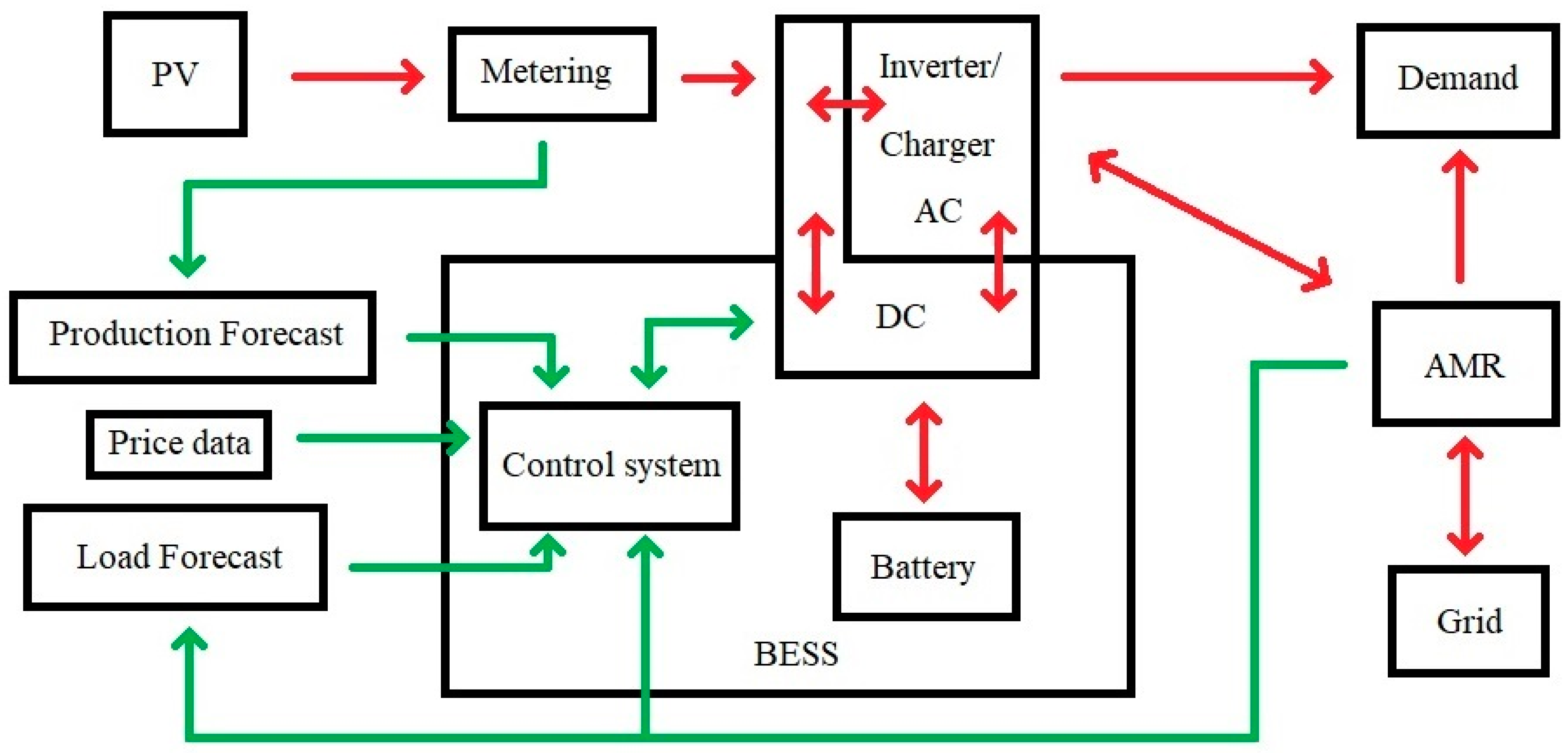
• This study is based on simulations using ordinary household customers’ demand data, with BESS added to the households’ electricity system. The simulation model is presented in Figure 1, which shows the directions of power flow and information data flow with red and green arrows, respectively. In the basic situation, PV power flows through the metering to the inverter, where it can go straight to the household to meet demand or to the BESS, and if the amount of produced energy is higher than the demand and the storage capacity is full, it can be fed to the grid and measured by automatic meter reading (AMR). If PV production cannot meet the energy need, it can be taken from the grid to meet the demand or to the BESS.
• Decision-making for battery charging and discharging occurs in the BESS control system. It controls the inverter/charger, which gives feedback on the battery conditions. Additionally, the control system includes a battery management system (BMS), which takes care of battery health. In the decision-making process, the control system uses the information from load and production forecast, upcoming electricity prices, and feedback from the charge controller and AMR. Load and production forecasts are based on weather forecasts and mathematical models, but these can be corrected based on PV production metering and data from AMR.

2.2.1. Household Electric System Model

In simulations, calculations are based on the initial household demand D, which is taken from measured data of actual electricity customers. The efficiency of inverter/charger η_inv affects the amount of energy, which is converted from direct current (DC) to alternating current (AC) or from AC to DC in an inverter/charger. In this study, the inverter efficiency and charger efficiency are assumed to be equal, and were both 98%. Additionally, battery charging and discharging causes losses on the DC side, but this is taken into account in the BESS model. PV production before the inverter/charger P_dc can go straight to the BESS, when inverter or charger efficiency does not affect it. Charger efficiency affects when the BESS is charged from the grid. The customer’s electricity bill is based on the measurements of AMR. Therefore, it is important to calculate the total demand measured by AMR, i.e., the demand from the grid perspective D_g, which is shown in Equation (4) [5]:

$$D_g=\{\begin{array}{cc}\frac{B_t-P_{dc}}{{\eta }_{inv}}+D& ||if B_t>P_{dc} \& B_t\ge 0\\ -{\eta }_{inv}\left(P_{dc}-B_t\right)+D& ||if B_t\le P_{dc} \& B_t\ge 0\\ {\eta }_{inv}\left(-B_t-P_{dc}\right)+D& ||if B_t<0\end{array}$$

(4)

where B_t is power flow to or from the BESS at time t. There are three equations for D_g because the equation is different if the battery is charged or discharged; additionally, if the battery is charged, the equation is different when charged energy is from PV or from the grid.

2.2.2. PV Model and Production Forecast

PV production P_pv is simulated by using a solar panel model, which is based on the nominal power of panels in standard test conditions P_STC and modeled global solar irradiance G_i. Differences in solar panel conditions are taken into account in Equation (5), which can be utilized in PV calculations [22]:

$$P_{pv}=C_v{P}_{STC}{G}_i\left(1-{\beta }_P\left(T_c-T_{STC}\right)\right)$$

(5)

where T_c is the solar cell temperature, T_STC is the standard test temperature (25 °C) and β_P is the solar cell power temperature coefficient (0.006). This model was verified in [5] with actual data from solar panels and the verification coefficient C_v was added (0.85). In the verification, polycrystalline silicon PV cells were used. This because the temperature of the solar panel cannot be known in simulations and outdoor temperature has to be used instead. Lower temperatures in Equation (5) increase production, so a coefficient is needed.

• Solar irradiance modeling is based on the Reindl model [23], which is a suitable model for diffuse irradiance with south-tilted solar panels in the conditions of Finland [22]. In the model, global irradiance G_i is the sum of beam irradiance G_b,i, diffuse irradiance G_d,i and reflected irradiance G_r,i. In modeling, it is most important to find out the time series of solar irradiation. How strong is the solar irradiation on solar panels at different times? Solar irradiance depends on the location on the Earth and the angles of tilted PV panels. In this study, modeled solar panels are tilted at a 45° angle to face south.
• The amount of PV production depends on the cloudiness. In the Reindl model, cloudiness is modeled by a brightening factor. In [24], a model for cloudiness probability in Finland is presented, and it is based on cloudiness changing randomly, but based on probability. The same time series of solar radiation was utilized in all simulations so that the circumstances are stable.
• In actual systems, production forecasting has been utilized in control systems. In this paper, where load forecast is under study, the production forecast is assumed as ideal so that this does not affect the results of load-forecasting effects.

2.2.3. BESS Model and Control System

In simulations, modeling of BESS is based on controlling the battery’s state of charge (SOC), which is the percentage of full battery E_max. In every moment when the battery is charged or discharged, the SOC changes, and it depends on the SOC at the previous moment. This can be formed with Equation (6) [5]:

$$SO{C}_t=100\frac{B_{eff}{B}_t}{E_{max}}+SO{C}_{t-1}$$

(6)

where SOC_t is the SOC at time t and SOC_t−1 is the SOC of the previous time step.

• Modeling of the battery type is undertaken via the efficiency of BESS B_eff, which is a combination of battery efficiency and power electronics efficiency, i.e., inverter/charger DC side in Figure 1. In this study, the efficiency of power electronics on the inverter/charger DC side η_dc was 99%. The battery type was a lithium iron phosphate (LFP, LiFePO₄) cathode with a graphite anode. A lithium-ion (Li-ion) battery was chosen because it is currently the best commercial solution for residential use, with high efficiency, developed technology, and long lifetime. The LFP cell type was chosen because it has good safety features and a very long lifetime, and the specific energy is not as high as other Li-ion batteries. It is a good choice for use in stationary home systems [25].
• Battery loss modeling was presented previously (e.g., in [8] by Koskela et al.). Loss depends on SOC and charging or discharging current. Very high or low SOC increases the loss and decreases the lifetime of the battery [26]. For this reason, the SOC limits of the battery were set at 25–95%. In Li-ion batteries, the internal serial resistance R_b is approximately constant between these SOC limits [27]. Therefore, the modeling of battery loss can be implemented with constant serial resistance of 0.026 Ω, which was studied for LFP cell type in [28] by Weniger et al. Charging and discharging losses are not equal, but when the battery use is cyclic, we can use average values for both processes. Charging and discharging efficiency η_c can be calculated with Equation (7):

$${\eta }_c=100\frac{V_b-I_c{R}_b}{V_b}$$

(7)

where V_b is the nominal voltage of the battery and I_c is the charging or discharging current. The value of B_t can be calculated by multiplying charging or discharging current by charging or discharging voltage V_b, which can be calculated by using Equation (8):

$$V_c=V_b-I_c{R}_b$$

(8)

• The control system in this paper makes it possible to combine multiple control targets, and it is a novel structure. The basic operation of the control system is that it tells the inverter/charger when to charge the battery and when to discharge. Optimization of the BESS for control targets based on minimizing customers’ electricity cost and its rules are described in Section 2.1. Firstly, if customers’ electricity cost depends on peak power, BESS is used to decrease maximum peak power. This is implemented via an algorithm which is presented in [8]. Based on the load forecasting, the control system calculates the power level that is possible to keep below by using BESS. If average power during a pricing period goes over this limit, the battery is discharged. Errors in load forecast can cause failure. Based on the amount of failure, a new target power level is determined.
• Secondly, if customers have their own PV production, maximizing self-consumption is the next target. If the battery is not used to decrease maximum peak power, it is discharged empty before the high production hours of midday. When it is necessary to do this depends on the production forecast and load forecast. Control systems estimate the potential needs of SOC levels in the battery based on the forecasts. The BESS stores the surplus energy from PV, which is used later when it is needed. Stored energy can be used immediately when consumption increases higher than production, but this can be delayed for other control targets.

Thirdly, if customers’ electricity cost depends on the market price of electricity, the control system charges the battery during low prices and discharges during high prices. Controlling is based on pairs of hours when electricity prices are different, as in [5]. Charging and discharging operations must follow one another, because the capacity of the BESS is limited, so with a reasonably sized BESS, typically charging and discharging cycles will be once a day. If other control targets are involved, other operations can be done, e.g., the BESS is charged from surplus PV production and discharging is timed for high price, or the BESS is discharged to decrease peak power and charged during low price. For these reasons, the control system uses some rules for market price control: the BESS is charged full at least during the three hours before the forecast power peak and is not charged during three hours before forecast surplus production. These rules are valid only if these control targets are involved. If there are any other restrictions, the control system finds the lowest and highest prices of the day and calculates whether it is profitable to use the BESS. The price difference must be so large that loss of storage will be exceeded.

2.3. Load Forecast

Load forecasting is used in the BESS control system. Because the use of load forecasting is the main study object in this paper, it is described in its own subsection. To compare the benefits of BESS caused by forecast-based control and errors in forecasts, forecast errors between 0% and 200% are studied. Ideal load forecasting corresponds to a forecast error level of 0%. When the load is forecast by using a load forecasting algorithm, the error level is 100% (i.e., the 100% error level corresponds to the actual load forecast). The range 0–200% is divided into 20% steps, and the absolute value of forecast error in every hour increases linearly from 0% to 200%.

In this study, forecasting error is modelled with two different methods: the basic method, where 100% forecast error is formed by using the load forecast algorithm, and the random method, where forecast error is formed randomly. For comparability, we try to keep the effectiveness at the same level as much as possible.

The basic load forecast is formed separately for every customer. The load forecast algorithm is based on the customer’s historical consumption data and the effect of outdoor temperature variation. The method was initially presented in [29] and was utilized in [8]. In load forecasting, the load profile of the day is formed from the average consumption of historical data from similar days, and the data are corrected with outdoor temperatures. Different types of days are weekdays, Saturday, Sunday and weekdays with public holidays. Additionally, days are divided for the four seasons throughout the year.

Mean absolute error (MAE) and root mean squared error (RMSE) are the best criteria for comparing the validity of the load forecast, and are used in the control of residential BESS [9]. In the random method, forecast errors are made by the random function in MATLAB^® R2018a by Matworks, so MAE and RMSE increase linearly, similar to the basic method. For ideal forecasting, normally distributed random errors are added, whose mean is zero and standard deviation increases 0.25 kW per 20%. With these parameters, RMSE is the same as in the basic method and MAE is also very close, as we can see from Figure 2.

2.4. Initial Data

This study used large datasets from different sources. The simulations need consumption data from customers and many kinds of electricity price data. Additionally, forecasting and PV production models need measured weather data. This subsection presents the data used in this study.

2.4.1. Consumption Data

• Customers’ consumption data were collected from actual customers between January 2014 and August 2016. The data were measured using customers’ AMR measurements from the area of one DSO in Finland. The total number of customers is 1525, but for the simulations 100 customers were selected randomly. These are basic household customers who live in detached houses, which mainly use electric heating, but the heating method can vary. The study group also included a few larger customers, such as farms. Data from 2015 were used for simulating the effects and the other data were used in load forecasting.

2.4.2. Electricity Prices

• A customer’s electricity bill in Finland consists of three parts: the ER part, the DSO part and taxes. Both the ER and DSO parts typically include basic charges (€/month), but customers cannot affect this by using the BESS, and for this reason basic charges are not included in the calculations in this study. The ER pricing used here is typical market prices based on tariffs in Finland, where hourly price is based on the day-ahead spot prices of the Nord Pool (Finland area prices) [21]. ERs add a 0.25 c/kWh margin to the market price, and if surplus energy from PV production is fed into the grid, ERs buy this energy for the same market price, but the margin is taken off. The margin forms the income of ERs.
• In this study, two distribution tariffs of a DSO are used. One is the power-based tariff, which is calculated for the same area where the group under study lives [7]. The power-based tariff includes an energy charge (0.72 c/kWh) and a power charge (7.23 €/kW/month). The power charge is based on the highest hourly average power of the month. The power-based tariff is used so that all possible BESS control targets are available. Because the power-based tariff is not yet widespread, the general distribution tariff in the same area is also used. The general tariff is widely used in Finland; it includes only an energy charge (5.21 c/kWh) [30]. All prices in this study include a 24% value added tax. In Finland, customers have to pay an electricity tax (2.79 €/kWh) on purchased energy. In this study, customers do not need to pay the DSO for surplus energy that is fed into the grid, and this is the typical situation in Finland.

2.4.3. Weather Data

• Load forecasting is based on outside temperature. Additionally, temperature and solar radiation data are used in the PV model. All weather data were taken from the open data of the Finnish Meteorological Institute [31]. Temperature data are measured hourly, and were measured at the Juupajoki weather station, which is the closest station to customers in the study group.

2.5. Study Cases

The effect of load forecasting was studied with different cases. There are three control targets, and all combinations of them were studied. The study cases are presented in Figure 3. The three basic control targets form study cases 1–3. These three basic targets are introduced earlier in Section 2.1., and in more detail: the case 1 in Section 2.1.1., the case 2 in Section 2.1.2., and the case 3 in Section 2.1.3. Cases 4–6 are the combinations of two of the basic targets and study case 7 is the combination of all targets. Combining of cases are introduces in Section 2.1.4. These seven cases are selected, because cases include all combinations, which make it possible to obtain cost savings for customers.

In every case, load forecast error varies between 0% and 200%. The ideal forecast corresponds to an error of 0%, and calculated forecast (i.e., load forecast, which is calculated as described in Section 2.3.) corresponds to an error of 100%. The load forecast for every customer was formed based on earlier consumption data and temperature. Absolute value and direction (forecasted value higher or lower than actual value) were calculated every hour. For every customer 11 load forecasts were formed, with error increasing from 0% to 200% with 20% steps. Simulations were made with all of these load forecasts. Based on the results of the simulations, it is possible to study the effect of the accuracy of load forecasts.

3. Results

3.1. Simulations with Power-Based Distribution Tariff

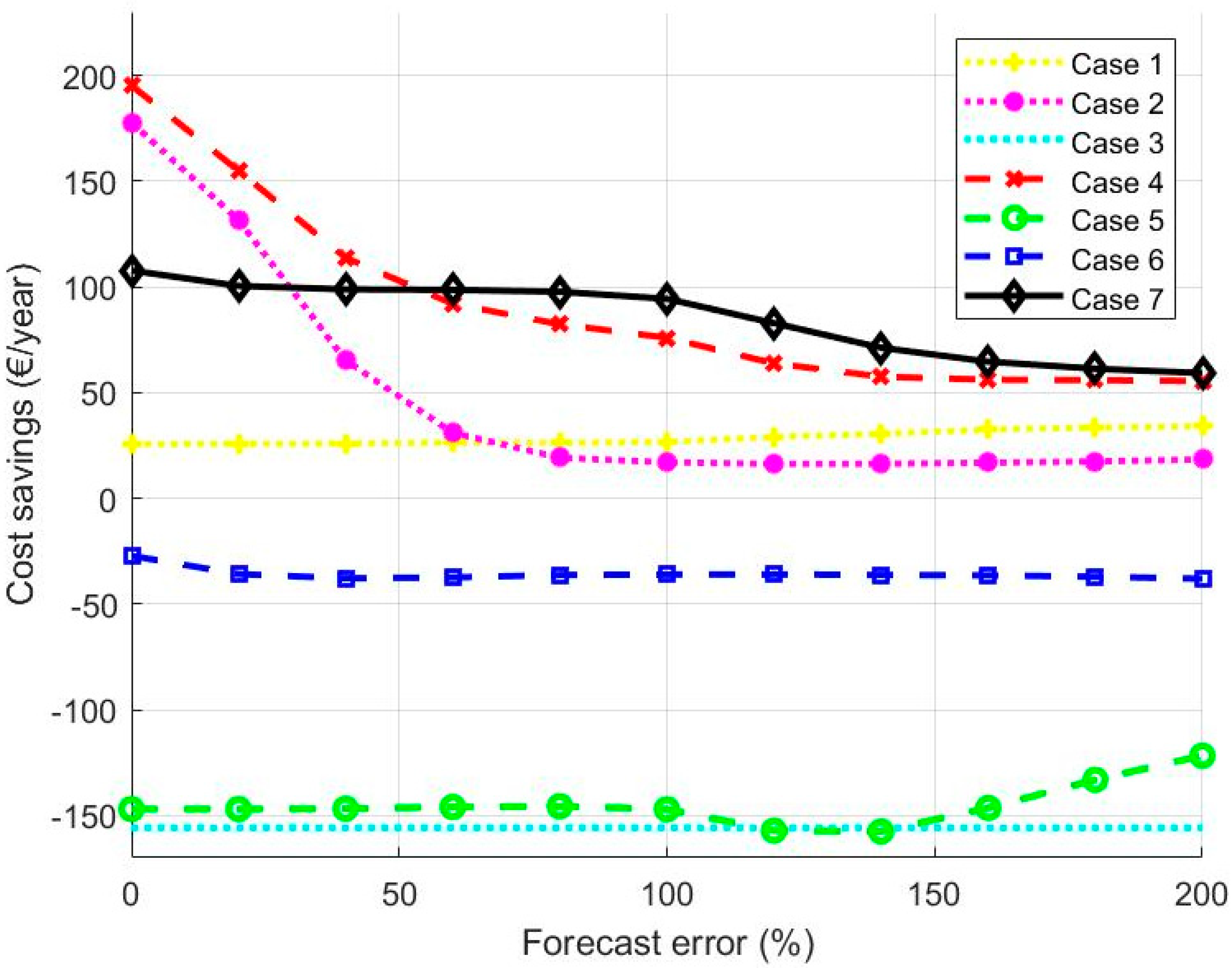
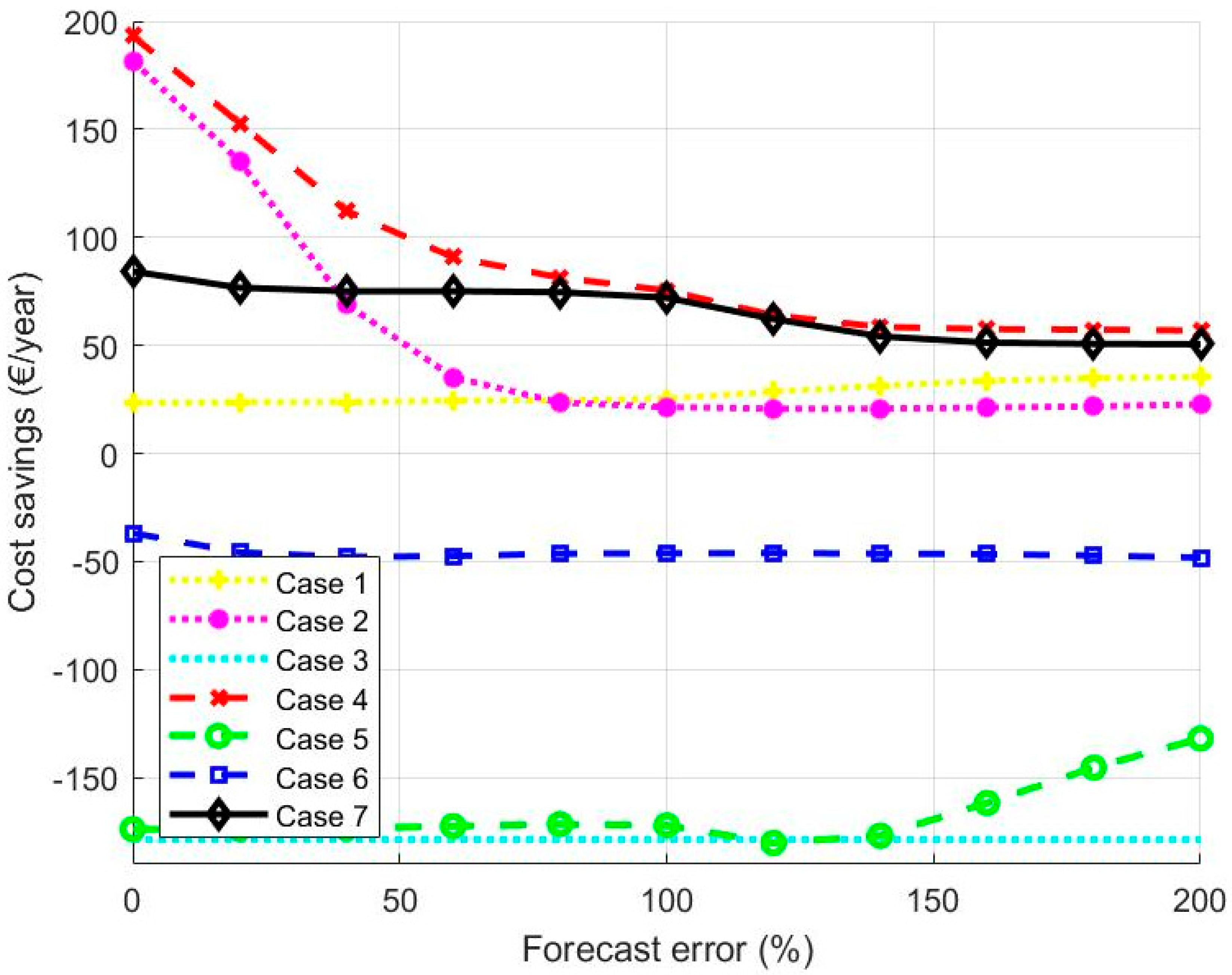
• In simulations, every customer had the added production of 3 kWp solar panels. The results are shown as average cost savings in the study group. Cost savings are presented as the function of forecast error. The results were calculated with the basic and random methods of modeling forecast errors. First, simulations were made with the power-based distribution tariff, where all possible cases (control targets) are meaningful.

3.1.1. Basic Method

The results of the simulations are presented in Figure 4, Figure 5 and Figure 6. Figure 4 presents the cost savings from total electricity costs per year. The cost savings from the distribution tariff and electricity tax are presented in Figure 5. Figure 6 shows the savings from market price-based cost paid to ERs.

• In case 1, the total cost savings increase marginally around the 100% forecast error, when the forecast error increases. This effect is caused by control inaccuracy. In the basic method of load forecasting, the direction of the error is the same at all error levels. Therefore, when the error increases, the control system increases its preparedness to store surplus energy. The same effect can be seen in case 5, which combines market price-based control (case 3) with case 1. In case 2, improved load forecasting strongly increases the cost savings when the forecast is very accurate. When the forecast error is over 80%, cost savings are almost constant. In case 3, the curve is flat. The negative number is leading from the increasing maximum peak power in market price-based control. Additionally, forecast errors do not notably affect the cost savings from market price-based control if decreased maximum peak power is not involved. The control system knows the whole time when high and low prices occur, so it uses BESS capacity maximally to shift the load from high price to low price, and it does not care about the load forecast.

When cases 1 and 2 were combined in case 4, the accuracy of the load forecast had a strong effect on the cost savings. Improving the load forecast increases cost savings significantly. In case 6, the load forecast must be very accurate after the improvement increases the cost savings. When all control targets are involved in case 7, the accuracy of the load forecast is very important around the 100% forecast error, but below 60% or over 140% the cost savings are stable. It is an important observation that with the current load forecast (100% forecast error), case 7, using all control targets, gives the highest cost savings.

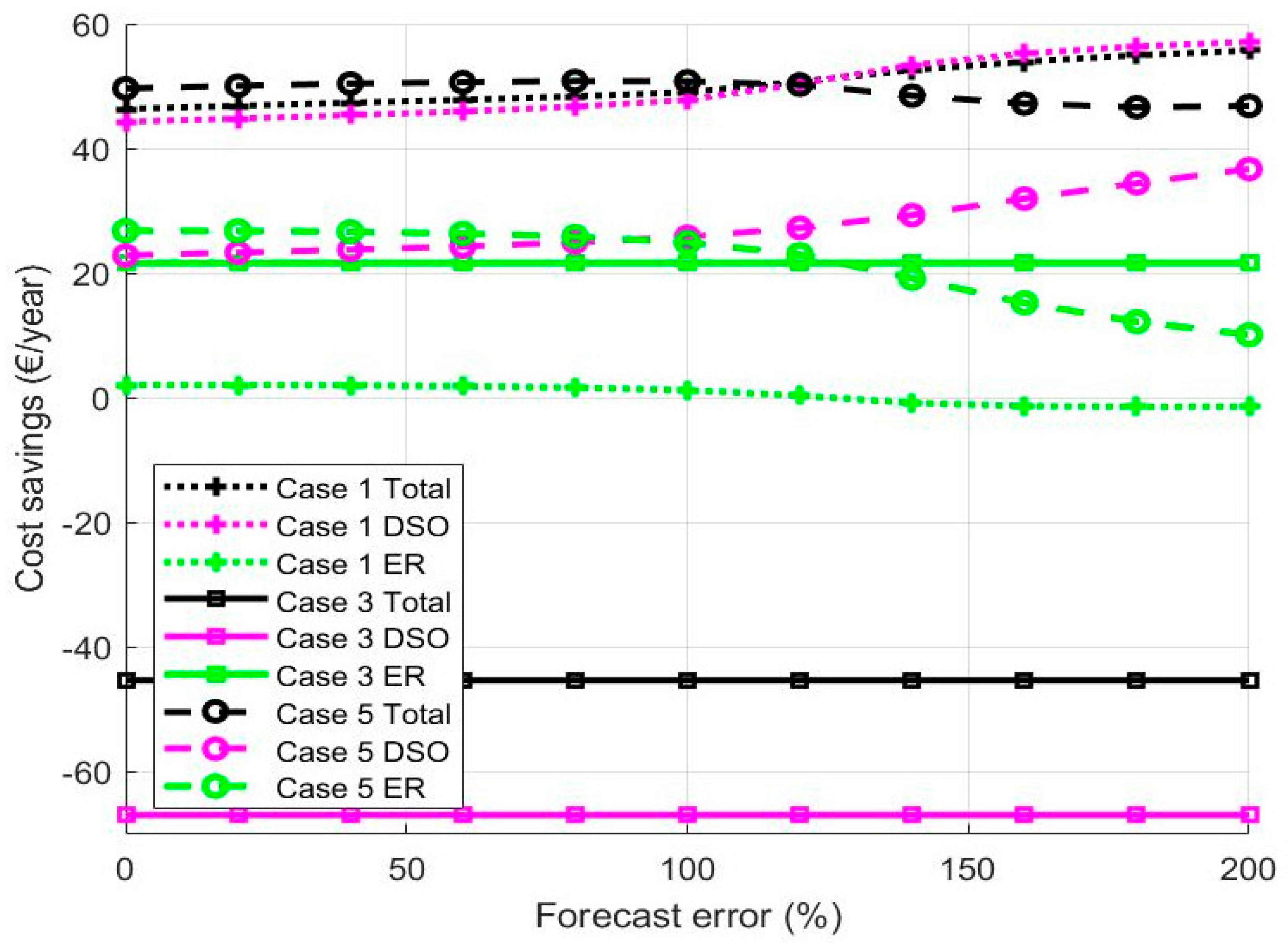
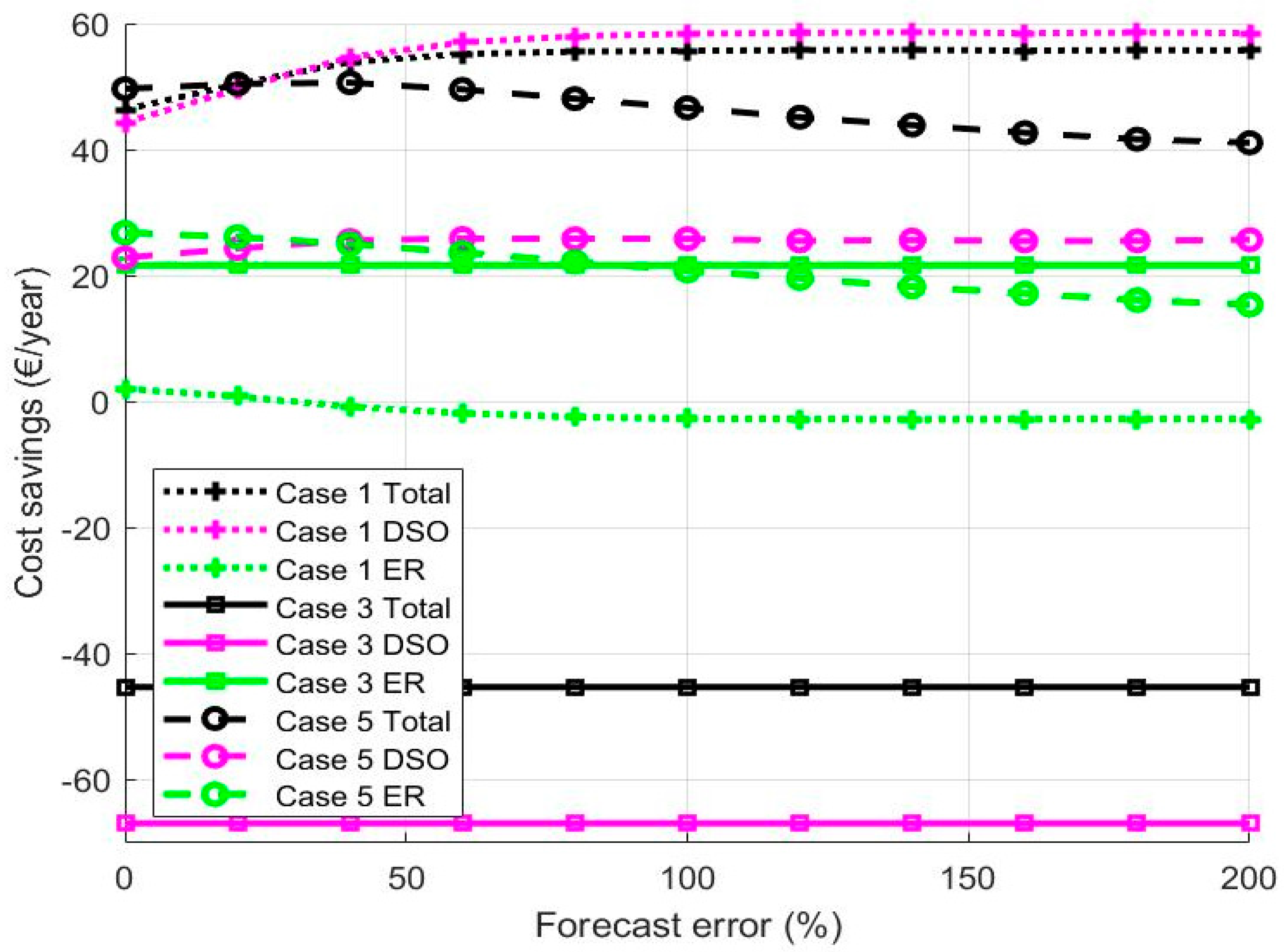
• Cost savings from the distribution tariff and electricity tax mostly affect total cost savings, as shown by the similar shape of curves in Figure 4 and Figure 5. Cost savings from the distribution tariff in cases where market price-based control is involved are lower than total cost savings. Additionally, in cases where decreased maximum peak power is involved, cost savings are higher.

The cost savings from ER contracts (Figure 6) shows that when the load forecast accuracy is increased from the current level, cost savings increase only marginally. Instead of a decreased load forecast, accurate cost savings are decreased dramatically in cases 5 and 7. These two cases give even higher cost savings from ER contracts than the clean market price control in case 3. The reason is that in case 3, control does not care when electricity is purchased and fed into the grid. In cases 5 and 7, feeding into the grid is limited when it is possible, because surplus energy is stored and grid feeding is not profitable. This makes it possible to obtain even higher cost savings when total electricity consumption is lower. Nevertheless, this needs very accurate load forecasting, and with bad load forecasts, cost savings drop lower.

3.1.2. Random Method

The results of the simulations with the random method of modeling forecast error are presented in Figure 7, Figure 8 and Figure 9. In the random method, the knowledge of high and low peaks in the load profile disappears when the forecast error increases. This can be seen when comparing the results in Figure 4, Figure 5, Figure 6, Figure 7, Figure 8 and Figure 9. With the random method the decrease of cost savings is smoother and continues almost the same throughout the whole forecast error range.

There are differences in how the forecast error modeling method affects the control targets. In case 2 with 100% error level, the random method gives higher cost saving than the basic method, and the same effect can be seen in case 4. This is because in the basic method, the same control errors repeat, because the forecast is based on historical data and temperature. In the random method, control errors also happen randomly, so the errors do not have as significant an effect. In case 7, which uses all control targets, almost all cost savings are lost with the random method at the 100% error level, and with the basic method, the cost savings are almost the same at the 0% error level.

For cost savings from ER contracts (Figure 6 and Figure 9) clear differences can be seen between forecast error modeling methods. The decrease of cost savings is smoother with the random method, but with the basic method higher cost savings can be reached at the 100% error level.

3.2. Simulations with General Distribution Tariff

In this subsection, the general distribution tariff is used. The power-based component of the tariff is not involved in the general distribution tariff, so it is meaningful to study only cases 1, 3 and 5, where decreased maximum peak power is not the target for control.

3.2.1. Basic Method

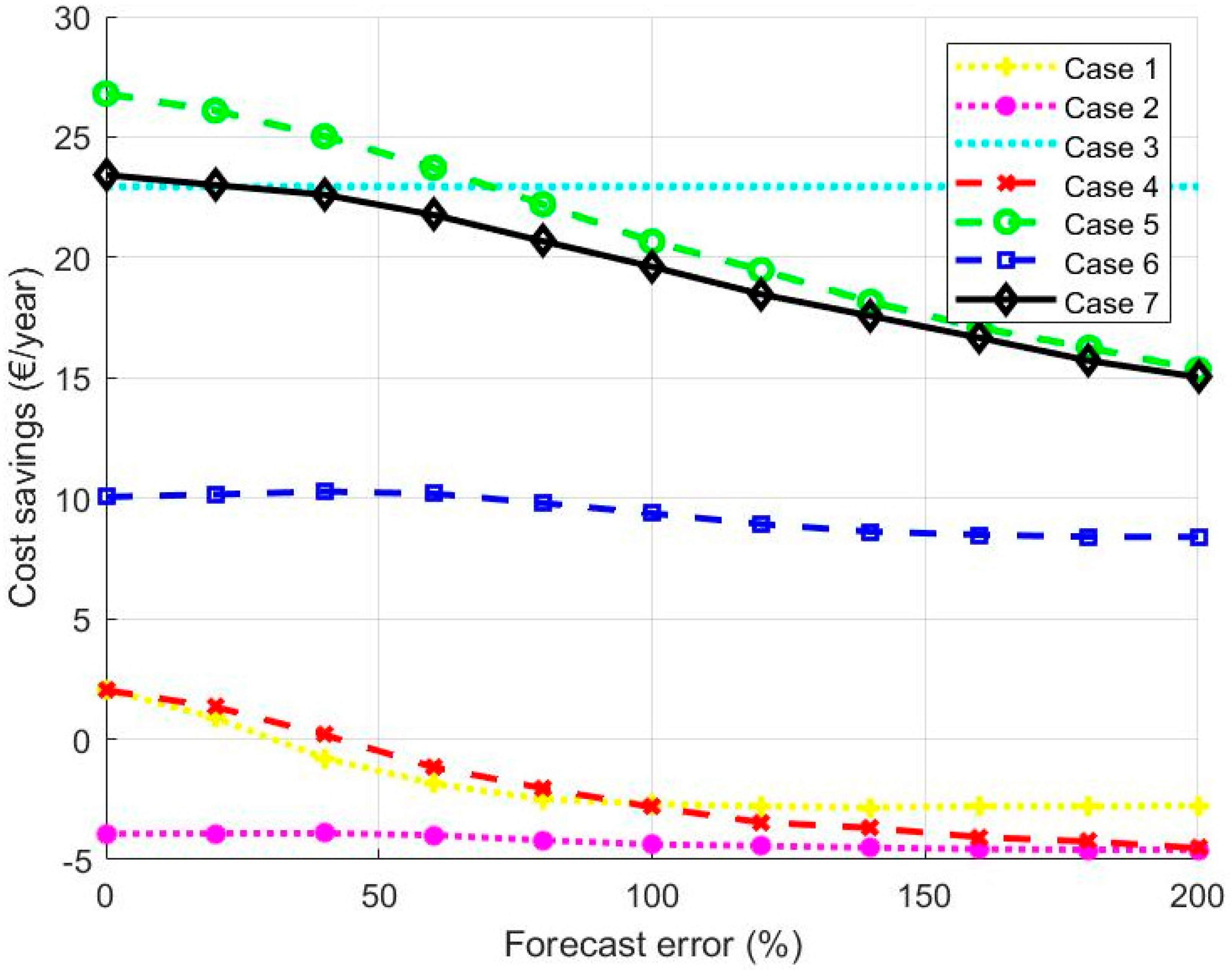
• When the basic method for modeling the error of load forecast is used, case 5 gives the highest cost savings before the error level of 120%. The results of this is shown in Figure 10. After that, as with the power-based tariff, the cost savings in case 1 increase and rise higher than in case 5. This is caused by the inaccuracy of the control system and the knowledge of the load profile in the basic method. The total cost savings in case 3 is not as negative as it is with the power-based tariff, but is still negative. This is because the control in case 3 does not care about the grid feeding from storage during high prices. This feature is involved in case 5, when the rise in cost savings is strongly positive. The main finding is that the effect of forecast error is not significant with the general distribution tariff and the differences between error levels are only marginal.

3.2.2. Random Method

• When the random method is used, the levels of cost savings are very similar to the basic method and the differences between error levels are only marginal. The results with the random method is shown in Figure 11. The biggest difference between basic and random methods is that the changes that happen after the 100% error level with basic the method happen before the 60% error level with the random method. When the random method is used, it seems that with current load forecast accuracy (100%), it is not profitable to use the combination of control targets (case 5) instead of case 1. However, when the basic method is used, the combination of control targets is the most profitable.

4. Discussion

The results of this study correspond with the expectations. Load forecasting is an important part of BESS control in domestic use when multiple control targets are used. Power-based distribution tariffs and market price-based ER contracts make it possible to use BESS for multiple control targets. When a general distribution tariff is used, the load forecast is not necessary. In simulations, it can be difficult to model the effect of load forecast errors. The modeling of forecast errors can be implemented by adding random errors to actual data. Forecast validity can be evaluated with error criteria such as MAE, RMSE or mean absolute percentage error (MAPE). However, this method does not correspond with real cases of load forecasting, which is done before BESS control. As the results of this study show, real load forecasts include information from the load profile, even if the error criteria are high. Therefore, the error criteria do not directly show the validity of the load forecast when it is used in the BESS control system.

Using BESS for only one control target can give some cost benefits, but using it for multiple targets can give even higher cost savings. In some cases, this also needs accurate load forecasting. This study shows that load forecasting is important, especially in cases 2, 4 and 7. In these cases, decreasing maximum peak power is involved. When both decreasing maximum peak power and storing surplus PV production are used, accurate load forecasting is very important. The profitability of BESS has been a barrier to its generalized domestic use. Higher cost savings from smart control systems makes it possible to increase profitability.

The results of this study are presented as average values of the study group. There are differences in cost savings between different customers, but average values show how this phenomenon behaves. When designing the control system of BESS for commercial application, this is expected to work with average customers. Even the load forecast is reasonable to individualize for different customers; it can be done by using the same principles. The results of this study show that it is more important for the load forecast to predict the load profile (i.e., when high and low peaks happen) than the actual accuracy of the forecast measured by error criteria.

The used optimization method was used partly before in [2,5,8], but all combinations are not used before. The benefits of this method are e.g., good functionality with different control targets, fast response with decent computation time and sensitivity for accuracy of load forecast. The used battery model corresponds to the modern Li-ion battery, which are available nowadays. Results of simulations are simulated in the Finnish electricity market environment, so the specifics of markets could cause the restrictions for the results. In other market environment, the cases and price levels could be different. There could be also other benefits from using BESS, e.g., the quality of electricity could improve, if BESS is also used for avoid black outs or stabilize the voltage level.

Simulations are made by using selected values in variables of modeling equations. The results of the study depends on the selected values. These values have been selected to correspond to the typical situation in a chosen environment. A small variation in these values causes only minimal effects on the results, when comparing these with the effect of load forecast error level. The results are not very sensitive for individual changes in these variables.

In the future, it will be worthwhile repeating the study with multiple ways of doing load forecasting. This study was conducted in the market environment of Finland, so future studies may be needed in different market environments. The results show that in many cases, the actual level of load forecasting is sufficient, but more accurate load forecasting could give even better cost savings and increase the profitability of BESS. More accurate load forecast is needed, when multiple control targets is used. In the future, there could be even more control targets which are studied in this paper and then the even more accurate load forecast could be useful. These are the focus of future studies.

References

1. Karjalainen, S.; Ahvenniemi, H. Pleasure is the profit—The adoption of solar PV systems by households in Finland. Renew. Energy 2019, 133, 44–52. [Google Scholar] [CrossRef]
2. Koskela, J.; Rautiainen, A.; Järventausta, P. Using electrical energy storage in residential buildings—Sizing of battery and photovoltaic panels based on electricity cost optimization. Appl. Energy 2019, 239, 1175–1189. [Google Scholar] [CrossRef]
3. Jiménez-Castillo, G.; Muñoz-Rodriguez, F.J.; Rus-Casas, C.; Talavera, D.I. A new approach based economic profitability to sizing the photovoltaic generator in self-consumption systems without storage. Renew. Energy 2020, 148, 1017–1033. [Google Scholar] [CrossRef]
4. Hirvonen, J.; Kayo, G.; Cao, S.; Hasan, A.; Sirén, K. Renewable energy production support schemes for residential-scale solar photovoltaic systems in Nordic conditions. Energy Policy 2015, 79, 72–86. [Google Scholar] [CrossRef]
5. Koskela, J.; Rautiainen, A.; Järventausta, P. Utilization possibilities of electrical energy storages in households’ energy management in Finland. Int. Rev. Electr. Eng. 2016, 11, 607–617. [Google Scholar] [CrossRef]
6. Honkapuro, S.; Haapaniemi, J.; Haakana, J.; Lassila, J.; Partanen, J.; Lummi, K.; Rautiainen, A.; Supponen, A.; Koskela, J.; Järventausta, P. Jakeluverkon Tariffirakenteen Kehitysmahdollisuudet ja Vaikutukset (Development Options for Distribution Tariff Structures); No. 65; LUT Scientific and Expertise Publications: Lappeenranta, Finland, 2017. (In Finnish) [Google Scholar]
7. Lummi, K.; Rautiainen, A.; Järventausta, P.; Heine, P.; Lehtinen, J.; Hyvärinen, M.; Salo, J. Alternative power-based pricing schemes for distribution network tariff of small customers. In Proceedings of the IEEE PES innovative smart grid technologies Asia (ISGT Asia), Singapore, 22–25 May 2018. [Google Scholar]
8. Koskela, J.; Lummi, K.; Mutanen, A.; Rautiainen, A.; Järventausta, P. Utilization of electrical energy storage with power-based distribution tariffs in households. IEEE Trans. Power Syst. 2019, 34, 1693–1702. [Google Scholar] [CrossRef]
9. Koponen, P.; Ikäheimo, J.; Koskela, J.; Brester, C.; Niska, H. Assessing and comparing short term load forecast performance. Energies 2020, 13, 2054. [Google Scholar] [CrossRef]
10. Goebel, C.; Cheng, V.; Jacobsen, H.-A. Profitability of residential battery energy storage combined with solar photovoltaics. Energies 2017, 10, 976. [Google Scholar] [CrossRef] [Green Version]
11. Ayuso, P.; Beltran, H.; Segarra-Tamarit, J.; Pérez, E. Optimized profitability of LFP and NMC Li-ion batteries in residential PV applications. Math. Comput. Simul. 2020, in press. [Google Scholar] [CrossRef]
12. Kuleshov, D.; Peltoniemi, P.; Kosonen, A.; Nuutinen, P.; Huoman, K.; Lana, A.; Paakkonen, M.; Malinen, E. Assesment of economic benefits of battery energy storage application for the PV-equipped households in Finland. J. Eng. 2019, 18, 4927–4931. [Google Scholar]
13. Hesse, H.C.; Martins, R.; Musilek, P.; Naumann, M.; Truong, C.M.; Jossen, A. Economic optimization of component sizing for residential battery storage systems. Energies 2017, 10, 835. [Google Scholar] [CrossRef]
14. Pilz, M.; Ellabban, O.; Al-Fagih, L. On optimal battery sixing for households participating in demand-side management schemes. Energies 2019, 12, 3419. [Google Scholar] [CrossRef] [Green Version]
15. Kharseh, M.; Wallbaum, H. How adding a battery to a grid-connected photovoltaic system can increase its economic performance: A comparison of different scenarios. Energies 2019, 12, 30. [Google Scholar] [CrossRef] [Green Version]
16. Schram, W.L.; Lampropoulos, I.; Van Sark, W.G.J.H.M. Photovoltaic system coupled with batteries that are optimally sized for household self-consumption: Assessment of peak shaving potential. Appl. Energy 2018, 223, 69–81. [Google Scholar] [CrossRef]
17. Litjens, G.B.M.A.; Worrell, E.; Van Sark, W.G.J.H.M. Economic bnefits of combining self-consumption enhancement with frequency restoration reserves provision by photovoltaic-battery systems. Appl. Energy 2018, 223, 172–187. [Google Scholar] [CrossRef]
18. Litjens, G.B.M.A.; Worrell, E.; Van Sark, W.G.J.H.M. Assesment of forecasting methods on performance of photovoltaic-battery systems. Appl. Energy 2018, 221, 358–373. [Google Scholar] [CrossRef]
19. Dongol, D.; Feldmann, T.; Schmidt, M.; Bollin, E. A model predictive control based peak shaving application of battery for a household with photovoltaic system in a rural distribution grid. Sustain. Energy Grids Netw. 2018, 16, 1–13. [Google Scholar] [CrossRef]
20. Beltran, H.; Ayuso, P.; Pérez, E. Lifetime expectancy of Li-ion batteries used for residential solar storage. Energies 2020, 13, 568. [Google Scholar] [CrossRef] [Green Version]
21. Nord Pool. Elspot Day-a-Head Electricity Prices. Available online: https://www.nordpoolgroup.com/Market-data1/Dayahead/Area-Prices/ALL1/Hourly/?view=table (accessed on 20 May 2020).
22. Vartiainen, E. A new approach to estimating the diffuse irradiance on inclined surfaces. Renew. Energy 2000, 20, 45–64. [Google Scholar] [CrossRef]
23. Reindl, D.T.; Beckman, W.A.; Duffie, J.A. Diffuse fraction corrections. Sol. Energy 1990, 45, 1–7. [Google Scholar] [CrossRef]
24. Hellman, H.-P.; Koivisto, M.; Lehtonen, M. Photovoltaic power generation hourly modelling. In Proceedings of the 2014 15th International Scientific Conference on Electric Power Engineering (EPE), Brno, Czech Republic, 12–14 May 2014. [Google Scholar]
25. Fernão Pires, V.; Romero-Cadaval, E.; Vinnikov, D.; Roasto, I.; Martins, J.F. Power converters interfaces for electrochemical energy storage system—A review. Energy Convers. Manag. 2014, 86, 453–475. [Google Scholar] [CrossRef]
26. Tremblay, O.; Dessaint, L.-A.; Dekkiche, A.-I. A generic battery model for the dynamic simulation of hybric electric vehicles. In Proceedings of the International Vehicle Power and Propulsion Conference, Arlington, TX, USA, 9–12 September 2007. [Google Scholar]
27. Parvini, Y.; Vahidi, A. Maximizing changing efficient of lithium-ion and lead acid batteries using optimal control theory. In Proceedings of the International American Control Conference, Chicago, IL, USA, 1–3 July 2015. [Google Scholar]
28. Weniger, J.; Tjaden, T.; Quasching, V. Sizing of residential PV battery system. Energy Procedia 2014, 46, 78–87. [Google Scholar] [CrossRef] [Green Version]
29. Mutanen, A. Improving Electricity Distribution System State Estimation with AMR-based Load Profiles; Tampere University of Technology: Tampere, Finland, 2018; p. 91. [Google Scholar]
30. Distribution Prices, Elenia. Available online: https://www.elenia.fi/sahko/siirtotuotteet (accessed on 20 May 2020).
31. Open Data, Finnish Meteorological Institute. Available online: httpt://en.ilmatieteenlaitos.fi/open-data (accessed on 20 May 2020).
Figure 1. Structure of household power system in simulation. Power flow is indicated by red arrows and information data flow by green arrows.
Energies 13 03946 g001
Figure 2. Error criteria with basic and random load forecast error models.
Energies 13 03946 g002
Figure 3. Study cases.
Energies 13 03946 g003
Figure 4. Total cost savings in function of forecast error in cases with basic method for modeling forecast error.
Energies 13 03946 g004
Figure 5. Cost savings from distribution tariff in function of forecast error in cases with basic method of modeling forecast error.
Energies 13 03946 g005
Figure 6. Cost savings from energy retailer (ER) contracts in function of forecast error in cases with basic method of modeling forecast error.
Energies 13 03946 g006
Figure 7. Total cost savings in function of forecast error in cases with random method for modeling forecast error.
Energies 13 03946 g007
Figure 8. Cost savings from distribution tariff in function of forecast error in cases with random method for modeling forecast error.
Energies 13 03946 g008
Figure 9. Cost savings from ER contracts in function of forecast error in cases with random method of modeling forecast error.
Energies 13 03946 g009
Figure 10. Cost savings in function of forecast error with general distribution tariff using basic method of load forecast error modeling in cases 1, 3 and 5.
Energies 13 03946 g010
Figure 11. Cost savings in function of forecast error with general distribution tariff using random method of load forecast error modeling in cases 1, 3 and 5.
Energies 13 03946 g011