Development of a Predictive Model for a Photovoltaic Module’s Surface Temperature


Abstract
1. Introduction
2. Previous Models for the Prediction of PV Module Surface Temperatures
3. Methodology
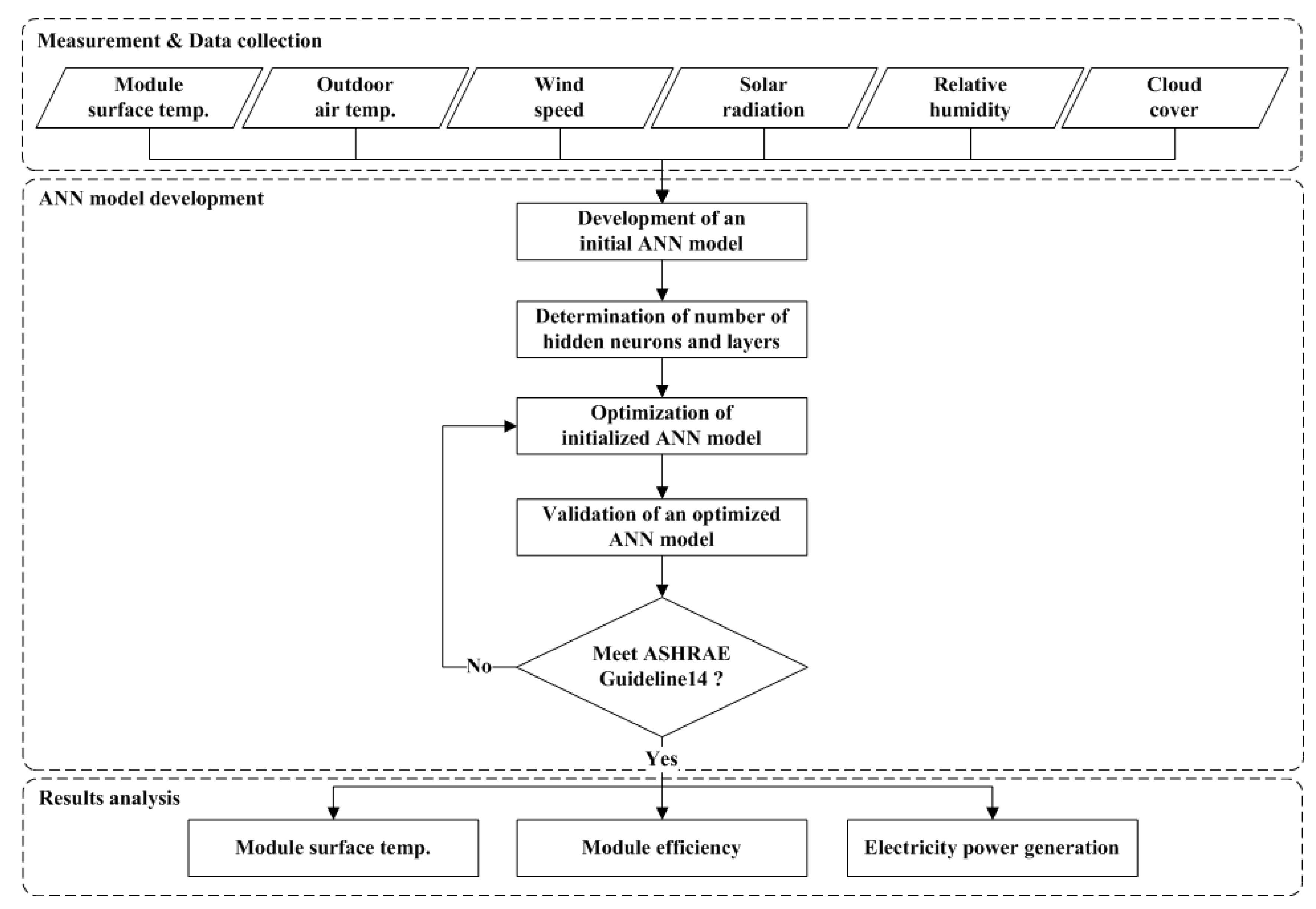
3.1. Overall Study Process
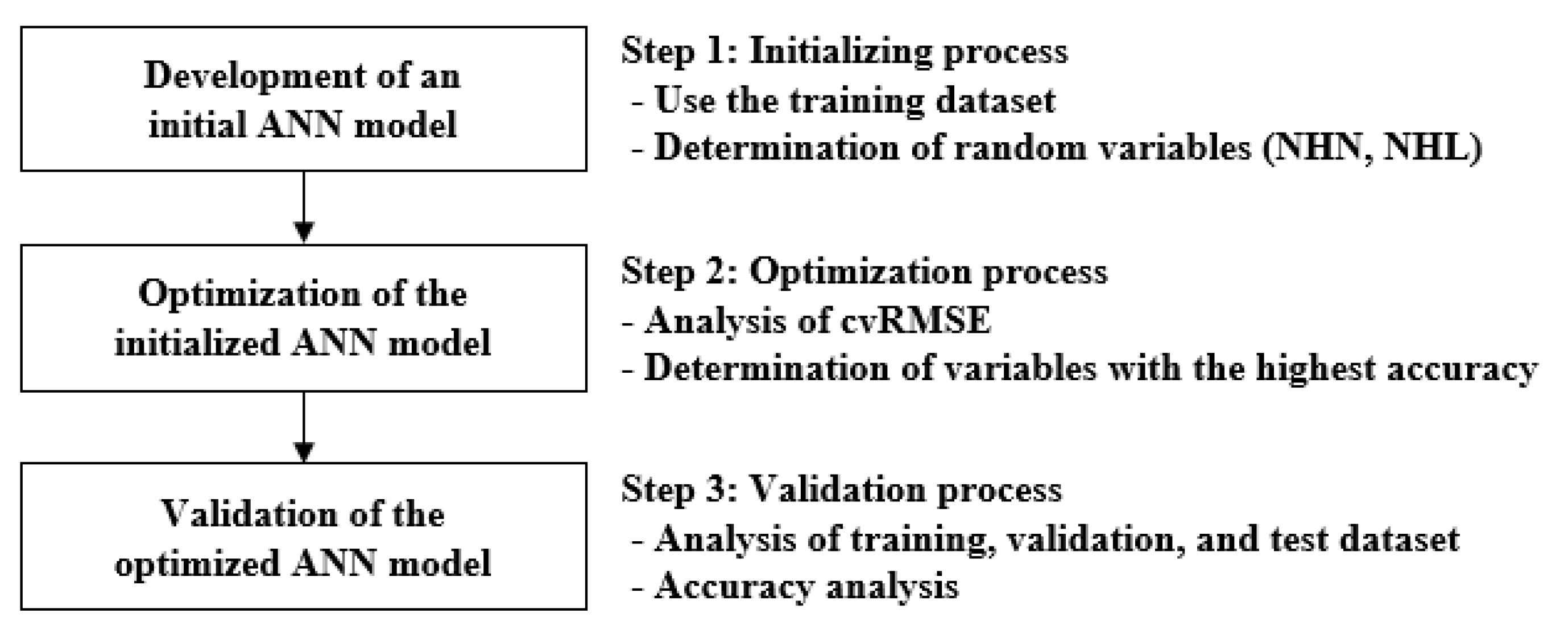
3.2. Development Process of the ANN Model
4. Results of the ANN Model
4.1. Development of an Initial ANN Model
4.2. Optimization of the Initial ANN Model
4.3. Validation of the Optimized ANN Model
5. Results Analysis and Discussion
5.1. Module Surface Temperature
5.2. Module Efficiency According to the Module Surface Temperature
5.3. Electricity Power Generation
6. Summary and Conclusions
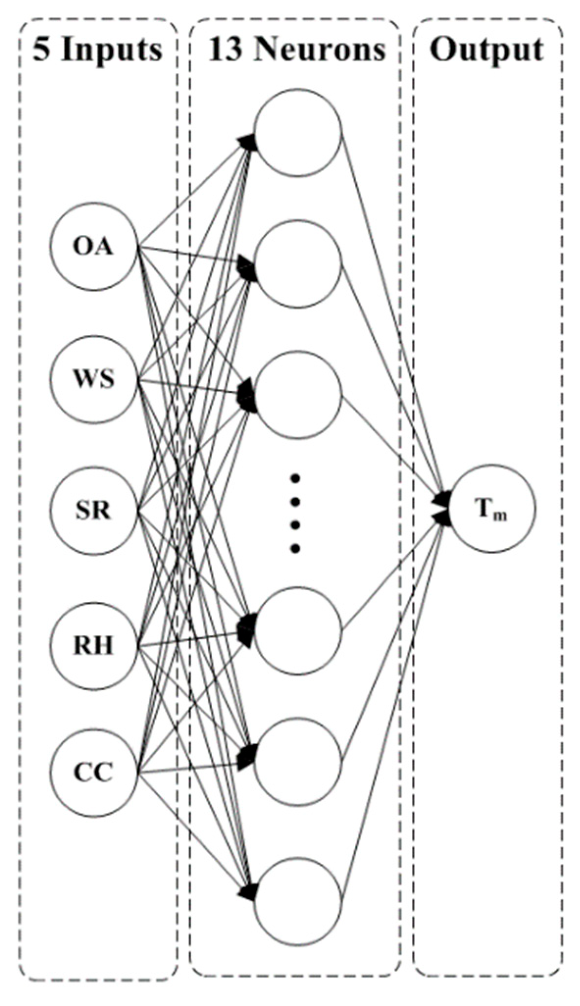
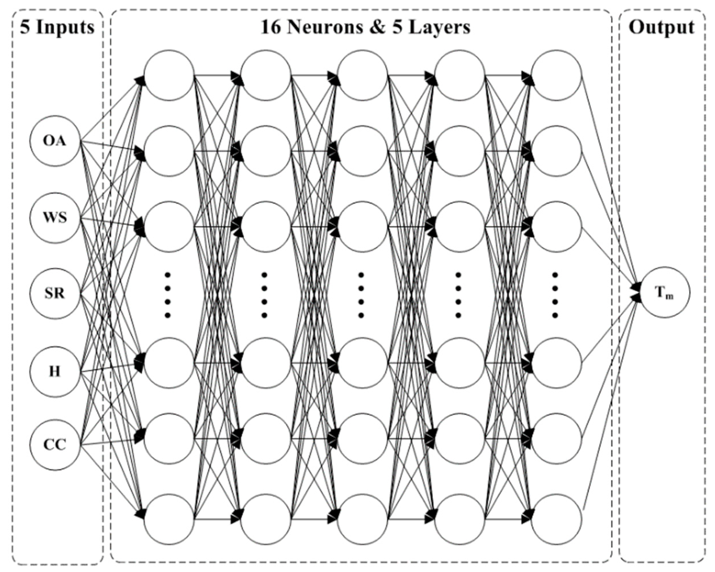
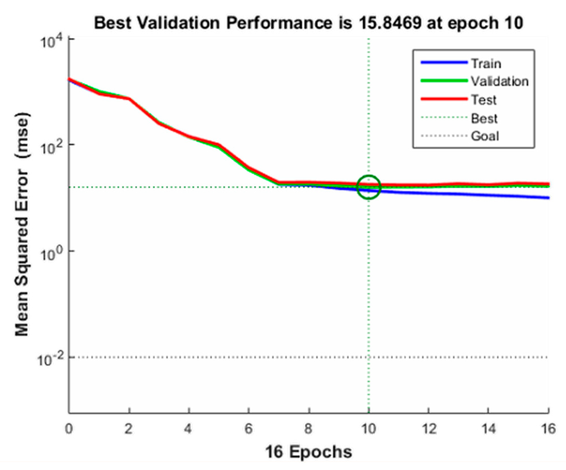
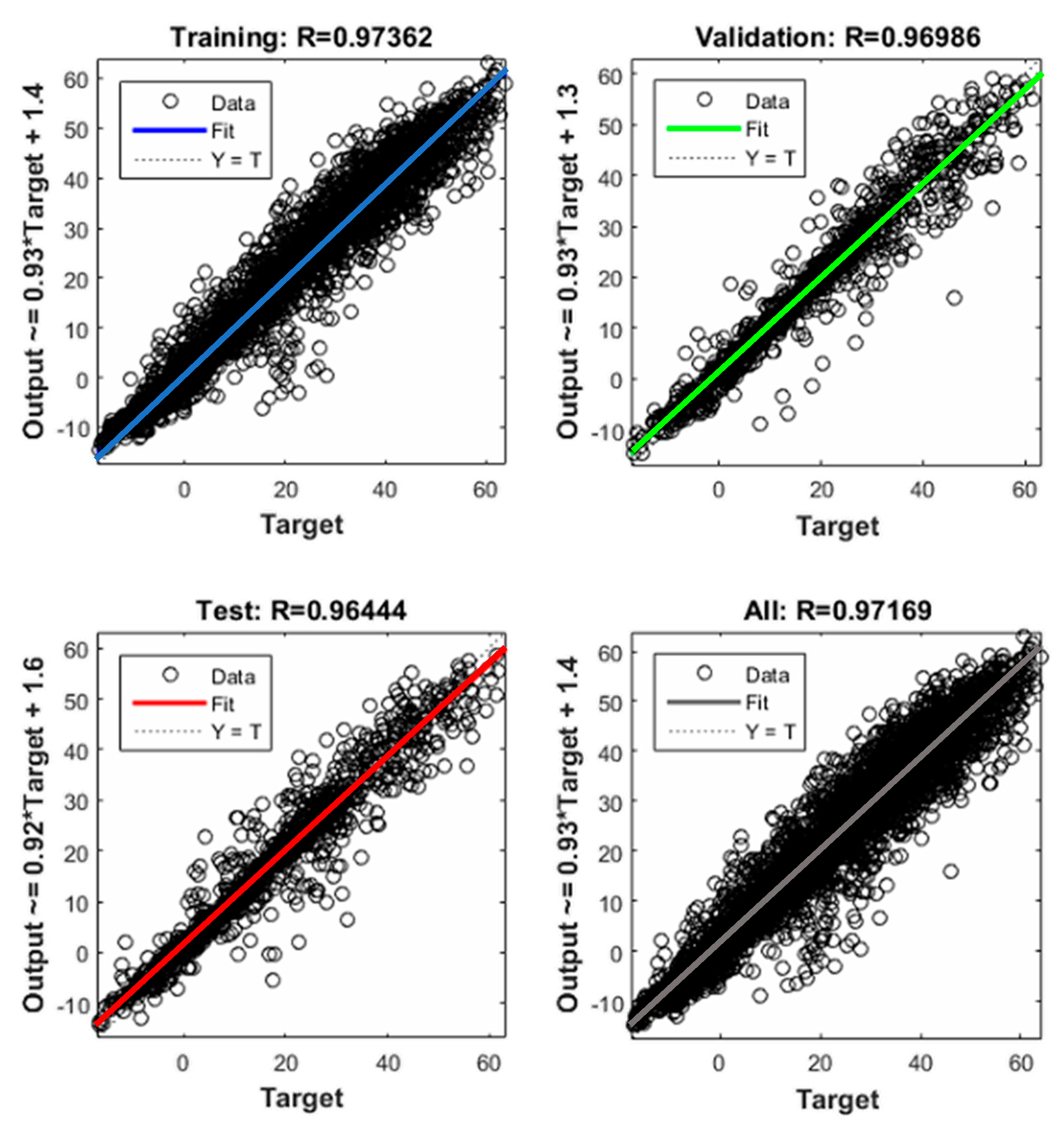
- The initial predictive model consisted of NHN = 13, NHL = 1, LR 0.3, and MC 0.3. The model’s cvRMSE was 22.00%. However, the predictive model’s accuracy was improved through an optimization process. The optimized predictive model showed the highest accuracy when NHN = 16, NHL = 5, LR 0.3, and MC 0.3. Under this configuration, the cvRMSE was 19.81%, an improvement of 2.19% over the initial predictive model. This model satisfied the recommendations specified in ASHRAE Guideline 14. In terms of the regression analysis results, the R2 value of the optimized predictive model was 0.97 for training, 0.97 for validation, 0.96 for test, and 0.97 overall. This shows that the optimized predictive model has high accuracy.
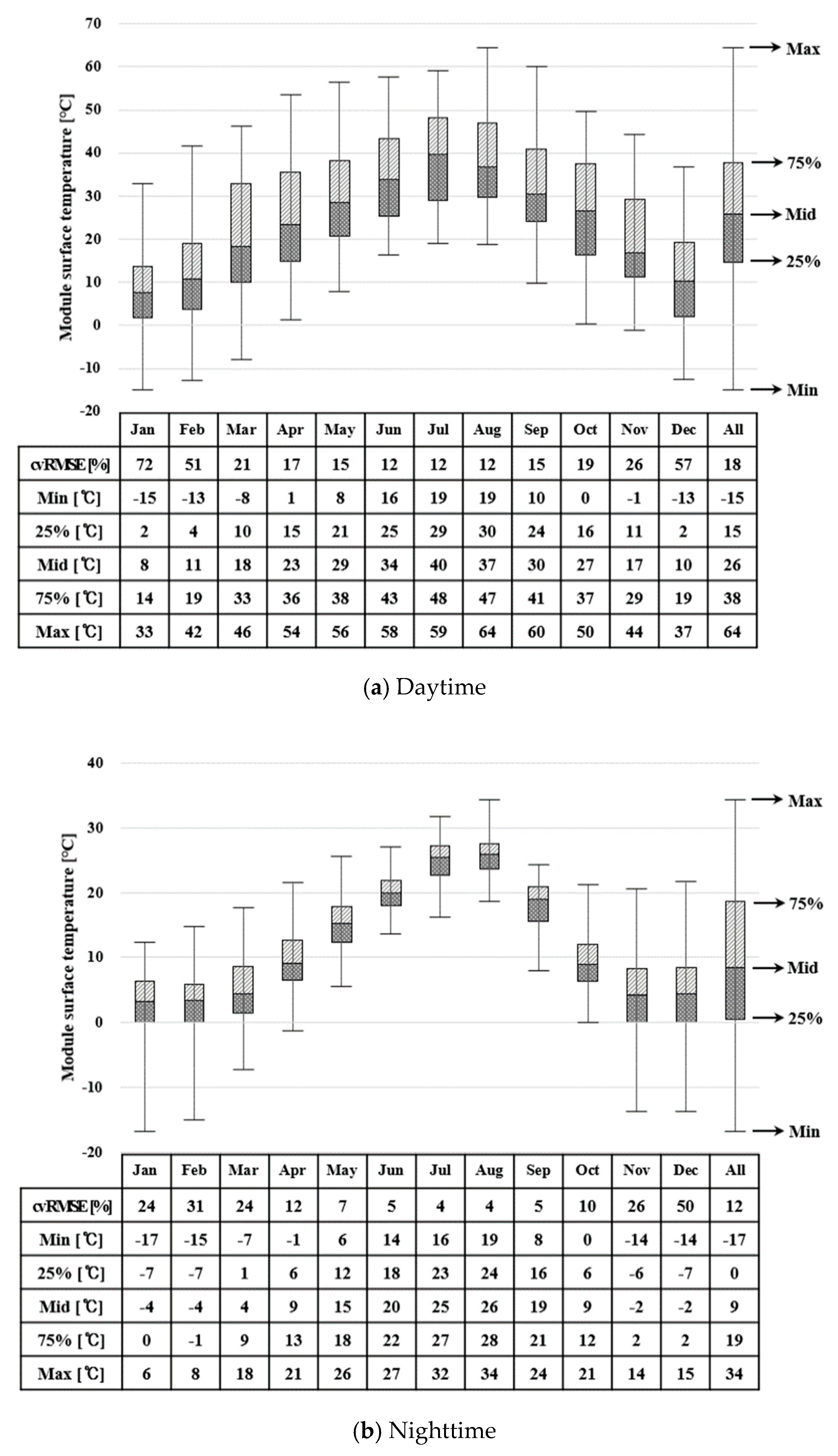
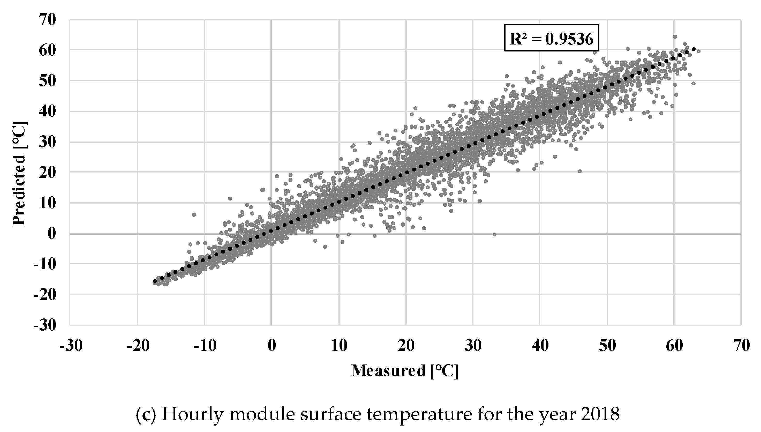
- The accuracy of module surface temperatures was higher during the nighttime than the daytime and higher in the summer than in winter. As a result of evaluating the annual cvRMSE, the daytime cvRMSE was about 18% and the nighttime cvRMSE was 12%. These results also satisfied the criteria specified in ASHRAE Guideline 14. In addition, the R2 value of the predicted annual module surface temperature was 0.95 when compared to the measured data. The model predicted the actual data with high accuracy. This shows that the developed model has high predictive performance.
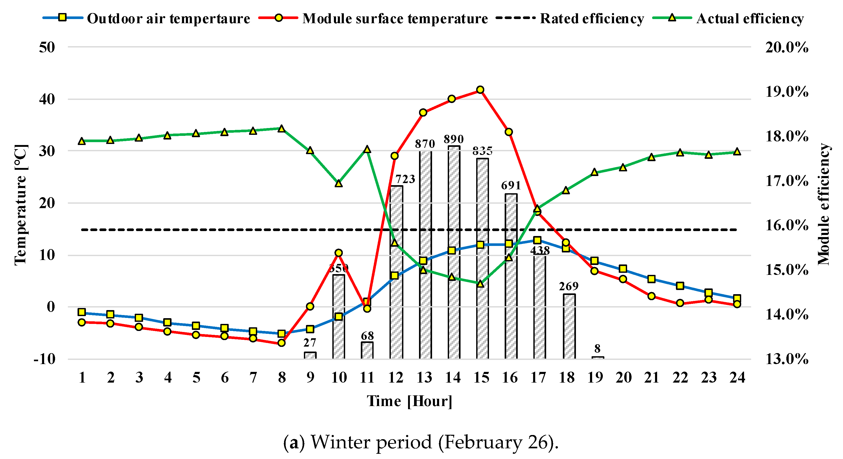
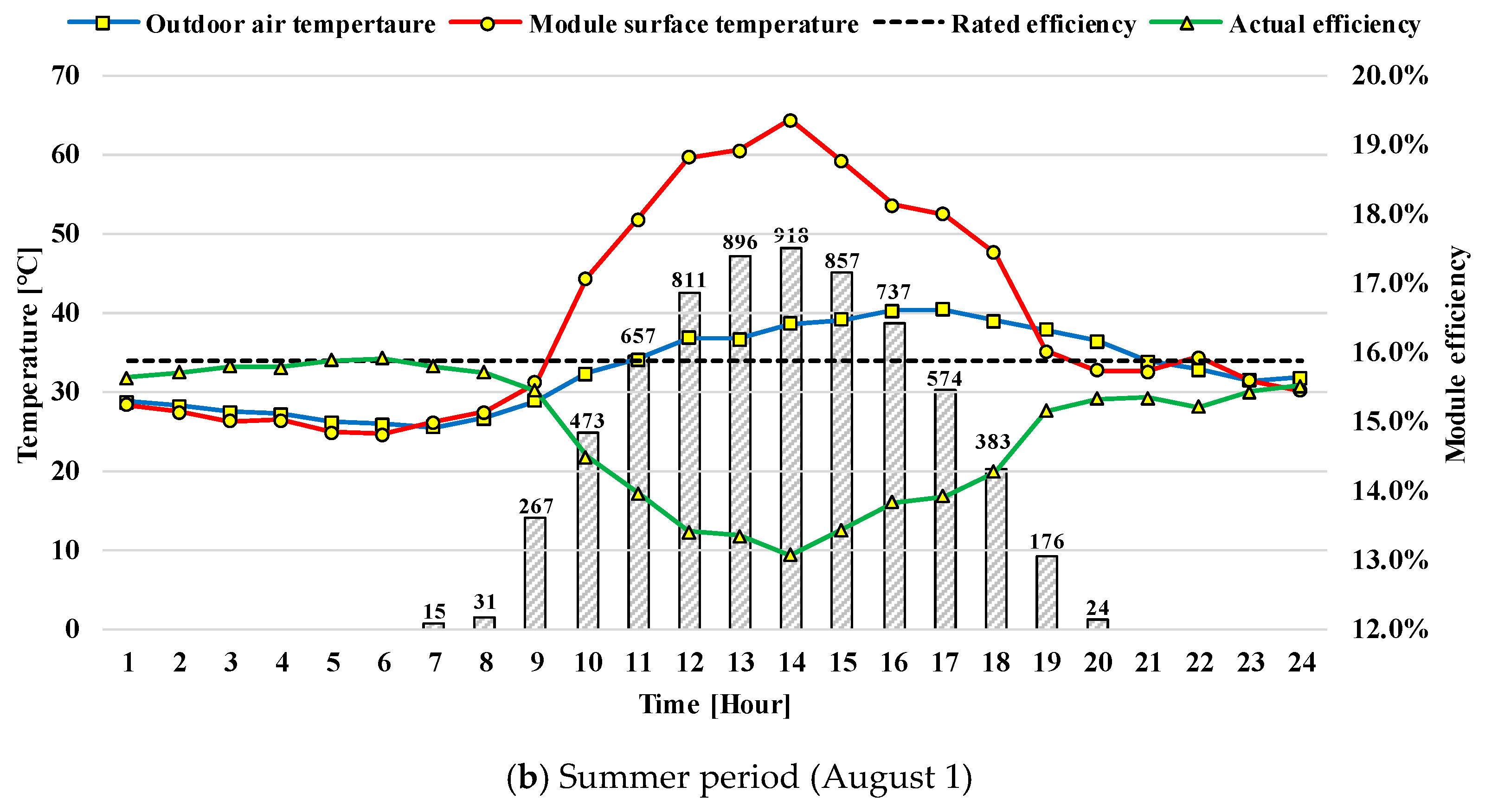
- As a result of analyzing efficiency according to module surface temperature changes, the efficiency decreased as the module surface temperature increased. When the module surface temperature rose during winter, the actual efficiency was about 14.7%, 1.2% lower than the rated efficiency. When the module surface temperature rose to 64.4 °C in the summer, the actual efficiency was about 13% and 2.7% lower than the rated efficiency. These results show that the module surface temperature may have adverse effects on the actual PV efficiency.
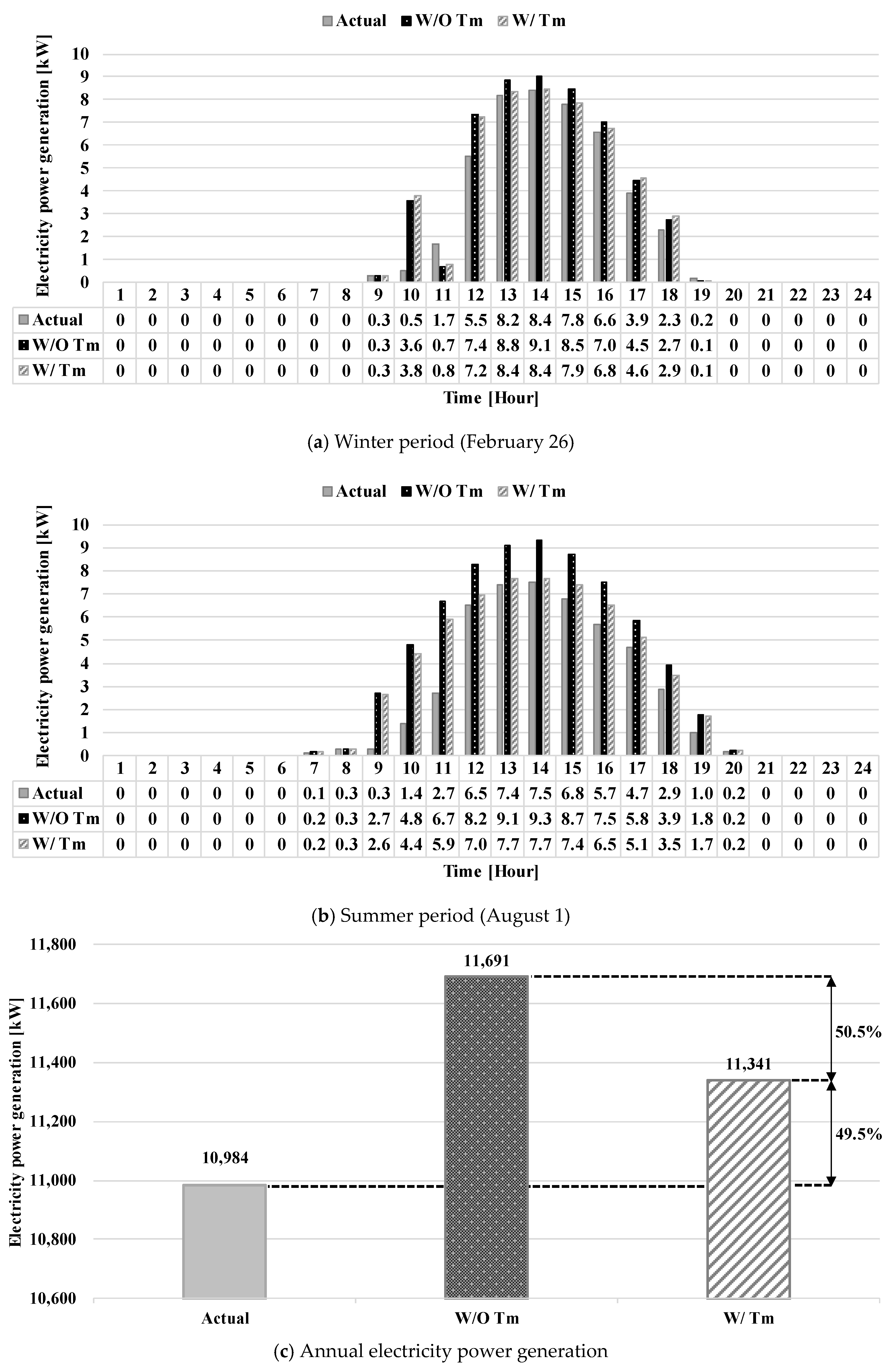
- In terms of annual power generation, W/Tm considering module surface temperature was closer to the measured power generation than W/O Tm without considering module surface temperature. In the case of relative error, W/Tm was about 50.5% lower than W/O Tm. That is, W/Tm was closer to the actual amount of power generated. These results will help calculate system capacity and prevent overdesign in the future.
Author Contributions
Funding
Conflicts of Interest
References
- Ministry of Land Infrastructure and Transport. Green Buildings Construction Support Act, MOLIT, 2008, Act No. 15728. Available online: https://elaw.klri.re.kr/kor_service/lawView.do?hseq=50008&lang=ENG (accessed on 10 June 2020).
- Ministry of Trade, Industry and Energy. Electricity Power Supply and Demand Trend, MOTIE. 2019. Available online: http://www.index.go.kr (accessed on 10 June 2020).
- Ministry of Trade Industry and Energy. Renewable Energy 3020, MOTIE. 2017. Available online: https://english.motie.go.kr (accessed on 10 June 2020).
- Fesharaki, V.J.; Dehghani, M.; Fesharaki, J.J.; Tavasoli, H. The effect of temperature on photovoltaic cell efficiency. In Proceedings of the 1stInternational Conference on Emerging Trends in Energy Conservation–ETEC, Tehran, Iran, 20–21 November 2011. [Google Scholar]
- Romary, F.; Caldeira, A.; Jacques, S.; Schellmanns, A. Thermal modelling to analyze the effect of cell temperature on PV modules energy efficiency. In Proceedings of the 2011 14th European Conference on Power Electronics and Applications, Birmingham, UK, 30 August–1 September 2011. [Google Scholar]
- Dubey, S.; Sarvaiya, J.N.; Seshadri, B. Temperature dependent photovoltaic (PV) efficiency and its effect on PV production in the world–a review. Energy Procedia 2013, 33, 311–321. [Google Scholar] [CrossRef]
- El-Adaw, M.K.; Shalaby, S.A. Effect of Solar Cell Temperature on its Photovoltaic Conversion Efficiency. Int. J. Sci. Eng. Res. 2015, 6, 1356–1384. [Google Scholar]
- King, D.L.; Kratochvil, J.A.; Boyson, W.E.; Bower, W.I. Field Experience with A New Performance Characterization Procedure for Photovoltaic Arrays. Presented at the 2nd World Conference and Exhibition on Photovoltaic Solar Energy Conversion, Vienna, Austria, 6–10 July 1998. [Google Scholar]
- Tamizhmani, G.; Ji, L.; Tang, Y.; Petacci, L. Photovoltaic Module Thermal/Wind Performance: Long-term Monitoring and Model Development for Energy Rating; National Renewable Energy Laboratory: Golden, CO, USA, 2003; pp. 936–939. [Google Scholar]
- Duffie, J.A.; Beckman, W.A. Solar Engineering of Thermal Processes, 4th ed.; Wiley: Toronto, ON, Canada, 2013; pp. 757–759. [Google Scholar]
- Skoplaki, A.G.; Boudouvis, J.A. A Simple Correlation for the Operating Temperature of Photovoltaic Modules of Arbitrary Mounting. Solar Energy Mater. Solar Cells 2008, 92, 1393–1402. [Google Scholar] [CrossRef]
- Schwingshackl, C.; Petitta, M.; Wagner, J.E.; Belluardo, G. Wind Effect on PV Module Temperature: Analysis of Different Techniques for an Accurate Estimation. Energy Procedia 2013, 40, 77–86. [Google Scholar] [CrossRef]
- Hassan, Q.; Jaszczur, M.; Przenzak, E.; Abdulateef, J. The PV cell temperature effect on the energy production and module efficiency. In Contemporary Problems of Power Engineering and Environmental Protection; Department of Technologies and Installations for Waste Management: Gliwice, Poland, 2016; Volume 33. [Google Scholar]
- Davis, M.W.; Fanney, A.H.; Dougherty, B.P. Prediction of building integrated photovoltaic cell temperatures. In Proceedings of the American Society of Mechanical Engineers Conference, Washington, DC, USA, 21–25 April 2001. [Google Scholar]
- Alonso Garcia, M.C.; Blaenzategui, J.L. Estimation of photovoltaic module yearly temperature and performance based on Nominal Operation Cell Temperature calculations. Renew. Energy 2004, 29, 1997–2010. [Google Scholar] [CrossRef]
- Mattei, M.; Notton, G.; Cristofari, C.; Muselli, M.; Poggi, P. Calculation of the polycrystalline PV module temperature using a simple method of energy balance. Renew. Energy 2006, 31, 553–567. [Google Scholar] [CrossRef]
- Kurtz, S.; Whitfield, K.; Miller, D.; Joyce, J.; Wohlgemuth, J.; Kempe, M.; Dhere, N.; Bosco, N.; Zgoena, T. Evaluation of high-temperature exposure of photovoltaic modules. Prog. Photovolt. Res. Appl. 2011, 19, 954–965. [Google Scholar] [CrossRef]
- Brano, V.L.; Ciulla, G.; Falco, M.D. Artificial neural networks to predict the power output of a PV panel. Int. J. Photoenergy 2014, 2014. [Google Scholar] [CrossRef]
- Ceylan, İ.; Erkaymaz, O.; Gedik, E.; Gürel, A.E. The prediction of photovoltaic module temperature with artificial neural networks. Case Stud. Therm. Eng. 2014, 3, 11–20. [Google Scholar] [CrossRef]
- Olukan, T.A.; Emziane, M. A comparative analysis of PV module temperature models. Energy Procedia 2014, 62, 694–703. [Google Scholar] [CrossRef]
- Ayvazogluyuksel, O.; Filik, U.B. Power output forecasting of a solar house by considering different cell temperature methods. In Proceedings of the ELECO 2017 10th International Conference on Electrical and Electronic Engineering, Bursa, Turkey, 30 November–2 December 2017. [Google Scholar]
- Kamuyu, W.C.L.; Lim, J.R.; Won, C.S.; Ahn, H.K. Prediction model of photovoltaic module temperature for power performance of floating PVs. Energies 2018, 11, 447. [Google Scholar] [CrossRef]
- Chayapathy, V.; Anitha, G.S.; Raghavendra, P.S.G.; Vijaykumar, R. Solar Panel Temperature Prediction By Artificial Neural Networks. In Proceedings of the 2019 4th International Conference on Recent Trends on Electronics, Information, Communication & Technology (RTEICT-2019), Bengaluru, India, 17–18 May 2019. [Google Scholar]
- Hegazy, A.; Shenawy, E.T.E.; Ibrahim, M.A. Determination of the PV Module Surface Temperature Based on Neural Network using Solar Radiation and Surface Temperature. ARPN J. Eng. Appl. Sci. 2019, 14, 494–503. [Google Scholar]
- MathWorks. Available online: http://www.mathworks.com (accessed on 10 June 2020).
- Marquardt, D.W. An Algorithm for Least-Squares Estimation of Nonlinear Parameters. J. Soc. Ind. Appl. Math. 1963, 11, 431–441. [Google Scholar] [CrossRef]
- Korea Meteorological Administration. Available online: https://data.kma.go.kr (accessed on 10 June 2020).
- S-Energy. SN72 Cell 1,000V Polycrystalline PV Module Catalogue, Korea. 2018. Available online: http://www.s-energy.com (accessed on 10 June 2020).
- Hargan, M.R. ASHRAE Guideline 14-2002 Measurement of Energy and Demand Savings; American Society of Heating Refrigerating and Air-Conditioning Engineers (ASHRAE) Inc.: Atlanta, GA, USA, 2002. [Google Scholar]
- Moon, J.W.; Kim, K.; Min, H. ANN-based prediction and optimization of cooling system in hotel rooms. Energies 2015, 8, 10775–10795. [Google Scholar] [CrossRef]


| Reference Number | Year | Objective | Location | PV Type | Methodology | Calculation Models | Input Parameters | Output Parameters | Accuracy | Analysis Parameters | |
|---|---|---|---|---|---|---|---|---|---|---|---|
| Experiment | Simulation | ||||||||||
| [14] | 2001 | Computation of the operating cell temperature | Maryland, US | Single Crystalline, Poly-Si, Si-Film, Triple-junction, A-Si | ○ | × | 1D steady state heat-transfer model | Solar radiation, Ambient temperature, Cell efficiency, Transmittance, Absorbance | Operating cell temperature | Relative error −12.1~10.6% | Cell temperature, Power |
| [9] | 2003 | Prediction of PV cell temperature | Arizona, US | Mono-Si, Poly-Si, A-Si, CIS, EFG-Poly-Si, CdTe | ○ | ○ | Linear regression model | Solar radiation, Ambient temperature, Wind speed, Wind direction, Relative humidity | Cell temperature | R2 = 0.943 | Cell temperature |
| [15] | 2004 | Estimation of PV module temperature and performance | Madrid, Spain | Semitransparent A-Si | ○ | ○ | Previous model | Solar radiation, Ambient temperature | Nominal operation cell temperature | Inaccuracy = ±3 °C | Cell temperature |
| [16] | 2006 | Development of a PV module temperature model | Ajaccio, France | Crystalline-Si | ○ | × | Modified model of previous model | Solar radiation, Ambient temperature, Wind speed, Convection coefficient | Cell temperature | RMSE = 2.24 °C | Cell temperature, Efficiency, Power |
| [17] | 2009 | Evaluation of PV cell temperature | Florida, US Colorado, US | Silicon Ribbon Module | ○ | × | Modified model of previous model | Solar radiation, Ambient temperature, Wind speed | Cell temperature | Unknown | Cell temperature |
| [18] | 2013 | Prediction of PV cell temperature | Palermo, Italy | Mono-Si, Poly-Si | ○ | ○ | Artificial neural network model | Power, Solar radiation, Weighting factor, Outdoor air temperature, Short circuit current, Open circuit voltage | Cell temperature | MAE ± 0.23 °C, ±0.11 °C | Cell temperature |
| [19] | 2014 | Prediction of PV cell temperature | Aegean, Turkey | Poly-Si | ○ | ○ | Artificial neural network model | System outlet air temperature, Solar radiation | Cell temperature | R2 = 0.99 | Cell temperature, Efficiency, Power |
| [20] | 2014 | Development of a 3D thermal model to predict the PV module temperature | Abu Dhabi, UAE | Poly-Si | ○ | × | 3D thermal model | Solar radiation, Ambient temperature, Wind speed, Heat loss coefficients | Cell temperature | RMSE < 1, MBE < 2 | Cell temperature, Power |
| [21] | 2017 | Forecasting of PV power considering cell temperature | Eskisehir, Turkey | Unknown | ○ | × | Previous model | Solar radiation, Ambient temperature, Wind speed, Convection coefficient | Cell temperature | RMSE = 2.23 °C MBE = 1.09 °C MABE = 1.82 °C | Cell temperature, Power |
| [22] | 2018 | Prediction of PV cell temperature | Hapcheon, Korea | Crystalline-Si | ○ | ○ | Multiple linear equation | Solar Radiation, Ambient temperature, Wind speed, Water temperature | Cell temperature | Relative error 2.06%, 4.40% | Cell temperature, Efficiency |
| [23] | 2019 | Prediction of PV cell temperature | Bengaluru, India | Unknown | ○ | ○ | Artificial neural network model | Solar radiation, Ambient temperature, Wind speed, Relative humidity, Panel temperature | Cell temperature | MAE = 0.9965 °C | Cell temperature |
| [24] | 2019 | Prediction of PV cell temperature | Cairo, Egypt | A-Si | ○ | ○ | Neural network model | Solar radiation, Ambient temperature | Cell temperature | 96% of accuracy | Solar radiation, Cell temperature |
| Parameters | Values |
|---|---|
| Outdoor air temperature (°C) | −16.2~40.4 |
| Wind speed (m/s) | 0~8.3 |
| Solar radiation (W/m2) | 0~1041.0 |
| Humidity (%) | 14.0~98.0 |
| Cloud cover (-) | 0~10.0 |
| Module surface temperature (°C) | −17.3~63.8 |
| Parameters | Values |
|---|---|
| Rated power (W) | 310 W |
| Voltage at Pmax (V) | 36.3 V |
| Current at Pmax (A) | 8.54 A |
| Warranted minimum Pmax (W) | 310 W |
| Short-circuit current (Isc) (A) | 8.96 A |
| Open-circuit current (Voc) (V) | 45.4 V |
| Module efficiency (%) | 15.89% |
| Operating module temperature (°C) | −40~+85 °C |
| Maximum system voltage (V) | 1000 V (IEC) |
| Maximum series fuse rating (A) | 15 A |
| Maximum reverse current (A) | 20.25 A |
| Power tolerance (W) | 0/+5 W |
| Measurements | Measurement Point | Type | Non-Stability |
|---|---|---|---|
| Solar radiation | Top side | Si-pyranometer (Class: C) | ±2% |
| Outdoor temperature | Back side | RTD (Class: B) | ±0.25% |
| Module surface temperature | Back side | RTD (Thin film) | ±0.5% |
| NHN | 8 | 9 | 10 | 11 | 12 | 13 | 14 | 15 | 16 | 17 | 18 | |
|---|---|---|---|---|---|---|---|---|---|---|---|---|
| NHL | ||||||||||||
| 1 | 23.39 | 22.02 | 22.18 | 21.57 | 22.62 | 22.35 | 21.85 | 21.33 | 21.42 | 21.42 | 21.66 | |
| 2 | 21.34 | 20.88 | 22.21 | 21.25 | 21.97 | 21.69 | 21.28 | 20.96 | 21.60 | 21.86 | 20.86 | |
| 3 | 21.17 | 21.71 | 21.43 | 21.41 | 21.30 | 21.43 | 21.23 | 20.61 | 22.10 | 20.83 | 21.04 | |
| 4 | 21.08 | 22.10 | 21.92 | 20.54 | 21.25 | 21.33 | 21.09 | 21.85 | 21.25 | 20.70 | 20.58 | |
| 5 | 21.58 | 21.09 | 23.41 | 20.90 | 21.10 | 21.61 | 21.12 | 21.98 | 19.81 | 21.65 | 20.93 | |
© 2020 by the authors. Licensee MDPI, Basel, Switzerland. This article is an open access article distributed under the terms and conditions of the Creative Commons Attribution (CC BY) license (http://creativecommons.org/licenses/by/4.0/).
Share and Cite
Jung, D.E.; Lee, C.; Kim, K.H.; Do, S.L. Development of a Predictive Model for a Photovoltaic Module’s Surface Temperature. Energies 2020, 13, 4005. https://doi.org/10.3390/en13154005
Jung DE, Lee C, Kim KH, Do SL. Development of a Predictive Model for a Photovoltaic Module’s Surface Temperature. Energies. 2020; 13(15):4005. https://doi.org/10.3390/en13154005
Chicago/Turabian StyleJung, Dong Eun, Chanuk Lee, Kee Han Kim, and Sung Lok Do. 2020. "Development of a Predictive Model for a Photovoltaic Module’s Surface Temperature" Energies 13, no. 15: 4005. https://doi.org/10.3390/en13154005
APA StyleJung, D. E., Lee, C., Kim, K. H., & Do, S. L. (2020). Development of a Predictive Model for a Photovoltaic Module’s Surface Temperature. Energies, 13(15), 4005. https://doi.org/10.3390/en13154005