A Real-Time Approach for Thermal Comfort Management in Electric Vehicles

Abstract

The HVAC system represents the main auxiliary load in electric vehicles, but passengers’ thermal comfort expectations are always increasing. Hence, a compromise is needed between energy consumption and thermal comfort. The present paper proposes a real-time thermal comfort management strategy that adapts the thermal comfort according to the energy available for operating the HVAC system. The thermal comfort is evaluated thanks to the “Predicted Mean Vote”, representative of passenger’s thermal sensations. Based on traffic and weather predictions for a given trip, the algorithm first estimates the energy required for the traction and the energy available for thermal comfort. Then, it determines the best thermal comfort that can be provided in these energetic conditions and controls the HVAC system accordingly. The algorithm is tested for a wide variety of meteorological and traffic scenarios. Results show that the energy estimators have a good accuracy. The absolute relative error is about 1.7% for the first one (traction), and almost 4.1% for the second one (thermal comfort). The effectiveness of the proposed thermal comfort management strategy is assessed by comparing it to an off-line optimal control approach based on dynamic programming. Simulation results show that the proposed approach is near-optimal, with a slight increase of discomfort by only 3%.

1. Introduction

Despite the rapid evolution of battery performance and recharging infrastructures, the penetration of electric vehicles (EVs) in road transportation remains hindered by their limited driving range and the consequent user’s fear of running out of battery. A lot of research effort is put into the battery itself, but another axis for improvement is to better anticipate the energy needs all over the trip and manage them according to the energy available in the battery. For instance, the heating, ventilating and air conditioning (HVAC) system is expected to maintain an acceptable thermal comfort inside the cabin regardless of the surrounding climatic conditions. Yet, in hot or cold weather conditions, its electric consumption may be quite significant and affect the vehicle driving range. Therefore, online energy management strategies are required in order to provide suitable tradeoff between the HVAC consumption and the passengers’ comfort. Such strategies can take great advantage of communication and context information, such as traffic and weather prediction, or charging stations map.

Thermal comfort is a complex concept, subject to a lot of work, but only recently car manufacturers have considered integrating this tricky notion in control and energy management. The issue is to minimize the HVAC energy consumption, while ensuring the passengers’ comfort. Approaches proposed in literature can be classified into two main categories: classical control approaches and optimal short-term management approaches. In the first category, fuzzy logic is the most used algorithm for thermal comfort management [1,2]. Some authors successfully customized passenger comfort by integrating a learning module [3,4]. In order to assess the effectiveness of these approaches, some authors have compared them to off-line optimal control methods like dynamic programming [5,6,7] and the minimum principle of Pontryagin [8]. In the second category of on-line approaches, the model predictive control model (MPC) is practically the only optimal algorithm that has been studied for HVAC control. For instance, in [1,9,10], the authors chose to minimize both discomfort and energy consumption, while in other works, the cost function also includes a third term related to further parameters, such as the temperature of the battery [11], the battery’s lifespan [12] and the air quality [13]. These approaches are interesting and effectively reach a trade-off between the different objectives set, yet, the following limitations can be noted: Firstly, they do not take into account the EV energy needs over the whole planned trip, which can lead to power shortages before reaching the destination. This is due to the chosen prediction horizon, which in general is a short horizon of the order of 1 to 30s [14,15]. In rare cases, the horizon can reach 10 min [16], 20 min [17] or even 30 min [18], but the entire trip horizon is not considered in order to adjust the passenger’s thermal comfort if needed. Secondly, the passengers’ thermal comfort is often modeled by a target temperature of 25 °C. Yet, this criterion can lead to thermal discomfort, with either hot or cold sensations, depending on the humidity and radiation temperature in the cabin [16]. Other on-line algorithms based on optimization have been used, like Stochastic Dynamic Programming (SDP) [19].

As mentioned earlier in this paper, the HVAC consumption may affect the driving range of the EV, especially in harsh weather conditions. In order to address this issue, we propose an on-line energy management strategy that provides, within the limits of available energy, an optimal thermal comfort to the passengers over a whole planned trip. If ideal thermal comfort cannot be provided at an acceptable energy cost (i.e., without causing power outages before reaching the destination), then it is reduced in order to allow the driver to arrive safely to the next charging point. The present study has been conducted for hot or moderate climates, but the proposed principles could also be extended to cold conditions.

In a former paper [20], we proposed to optimize the global passenger’s thermal comfort over a trip, while taking into account the actual quantity of energy available for operating the HVAC system. The idea was that, if there is not enough embedded energy for both traction and thermal comfort for the planned trip, the thermal comfort should be diminished in order to save energy and allow the vehicle to reach its final destination. In some situations, it may be wiser to consider slowing down the vehicle in order to allow better thermal comfort. After modeling the powertrain and the HVAC system, the problem was formalized as an optimal control problem and solved off-line, using dynamic programing. While the results were promising and validated the principle of thermal comfort and energy management, the computation cost of dynamic programing is still too high (curse of dimensionality [21]) for an implementation in an on-board computer, for real-time energy management.

In the present paper, we propose a real-time approach, based on on-line estimation of the energy required for traction and thermal comfort throughout the planned trip, given traffic and weather predictions. These estimators are built off-line and used on-line, first to determine the quantity of energy available for thermal comfort, and then to adjust the thermal comfort accordingly, in real time. An important point of this work is that we model the thermal comfort by the predicted mean vote criterion (PMV), proposed by Fanger in [22], and that reliably reflects the human perception of temperature and humidity [23]. The proposed approach was tested for 4000 test-cases and compared to an optimal dynamic programming-based approach [20]. The results show that the proposed real-time control is able to adjust the thermal comfort in case of low battery state-of-charge, and provides a near optimal tradeoff between energy consumption and thermal discomfort.

The contributions of the work presented in this paper may be summarized as follows: (i) estimation of the traction energy for a given planned trip modeled by macroscopic traffic indicators, (ii) estimation of the HVAC energy for given weather conditions over the planned trip, (iii) integration of the PMV as an estimator for passenger thermal comfort, (iv) real-time control approach for long horizon thermal comfort management, and (v) extensive simulations of the proposed real-time control for different climate and traffic scenarios, and comparison with an optimal dynamic programming approach.

The remainder of this paper is organized as follows: Section 2 describes the HVAC, powertrain and the battery sub-systems. Section 3 presents the proposed real-time thermal comfort management approach. Firstly, an overview of the algorithm is presented together with the thermal comfort criterion. Then, the powertrain and the HVAC system power estimators are presented. Finally, the algorithm of the thermal comfort management strategy is given. Section 4 presents results for a large number of weather and traffic scenarios. The accuracy of the HVAC system consumption estimator is analyzed. The near-optimality of the proposed approach is assessed by comparing it against an optimal dynamic programming approach. Section 5 summarizes the conclusions of the present work and gives some perspectives for further works.

2. System Description and Modeling

The studied system consists of three sub-systems: the HVAC system, the powertrain and the battery, which provides energy to the powertrain for traction and to the HVAC system for thermal comfort. The present work deals with thermal comfort in moderate and hot climates, and we will consider only the cooling function of the HVAC system.

2.1. HVAC System Description and Modeling

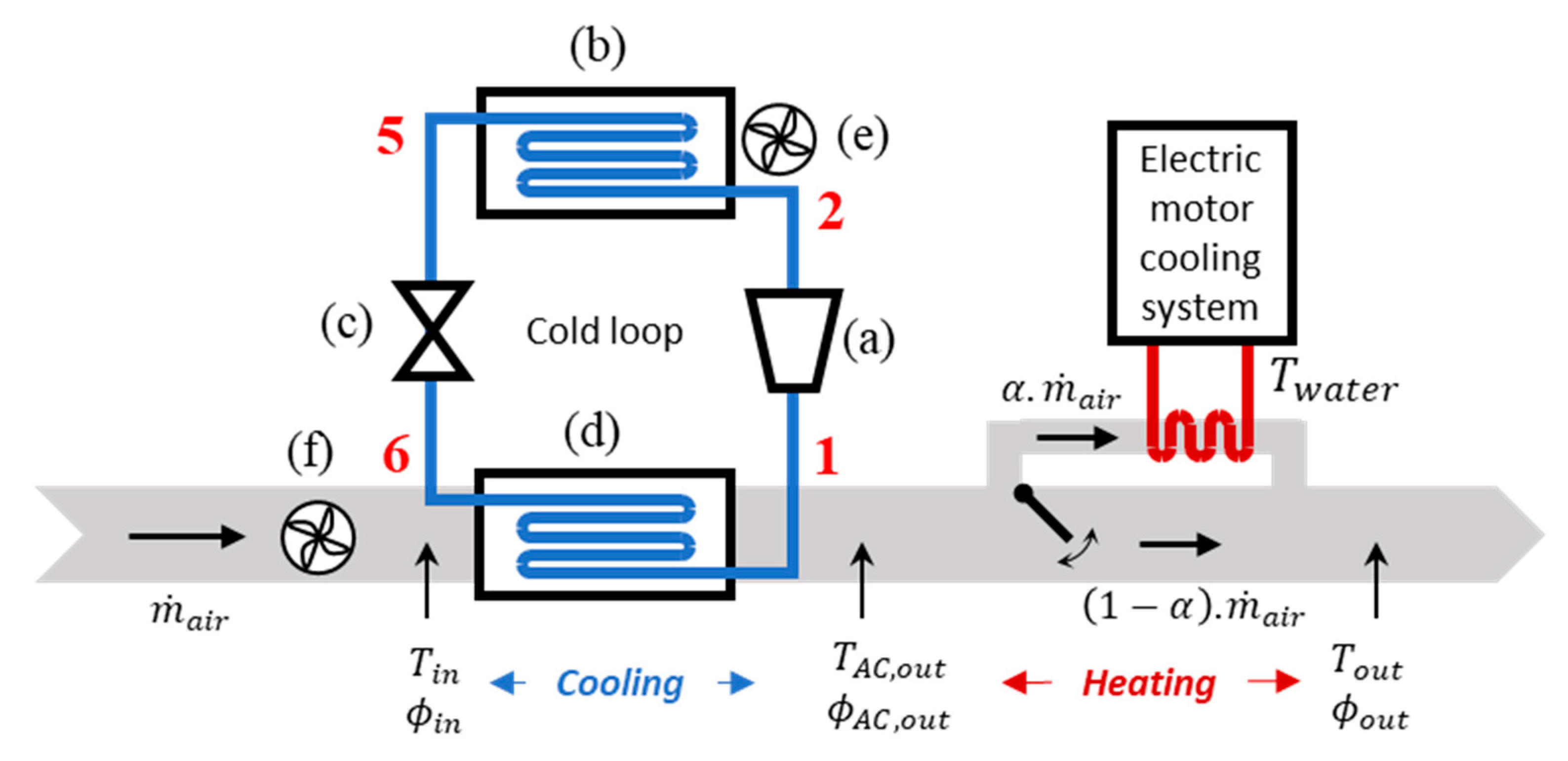
Figure 1 shows a schematic drawing of the HVAC system. It consists of three main components: one is the ventilation circuit (grey loop) that blows conditioned air in the cabin, and the two others are the cooling and heating systems (resp. blue and orange boxes) that exchange thermal power with the blown air in order to adjust its temperature and humidity.

As depicted, the outside air flow is mixed with a certain amount of recirculated cabin air and blown by a fan into the ventilation system. The air is firstly cooled and dried up by yielding thermal energy to the cold loop of the cooling system, through the evaporator, as detailed in Figure 1. At this stage, it is too cold to be directly blown into the cabin and it needs to be warmed up in the heating system. This can be done at a zero energetic cost by exchanging with the cooling system of the traction motor.

Using the notations defined in Figure 1, the ventilation sub-system can be modeled as follows. After mixing, the temperature $T_{in}$ and the specific humidity ${\varphi }_{in}$ of the air (mass of water vapor present in a unit mass of moist air) are given by (1) and (2), where $\beta$ is the recycling ratio:

$$T_{in}=\beta ·T_{cab}+\left(1-\beta \right)·T_{ext}$$

(1)

$${\varphi }_{in}=\beta ·{\varphi }_{cab}+\left(1-\beta \right)·{\varphi }_{ext}$$

(2)

The air flows through the cooling and heating sub-system, after which the temperature and specific humidity are denoted by $T_{out}$ and ${\varphi }_{out}$, respectively. The HVAC system enables controling these quantities, as it will be described later on in this section.

The conditioned air is blown into the cabin, and the cabin temperature evolution is governed by (3), where $C_{cab}$ is the cabin thermal capacitance (including walls and seats). ${\dot{Q}}_{ext}$ is the convective heat follow rate exchanged with the outside through vehicle body leakages. ${\dot{Q}}_{flow}$ corresponds to the heat exchange due to the air circulation. ${\dot{Q}}_w$ represents the heat flow rate, which is exchanged with the cabin walls, windows and windshield:

$$C_{cab}\frac{d{T}_{cab}}{dt}\left(t\right)={\dot{Q}}_{ext}\left(t\right)+{\dot{Q}}_{flow}\left(t\right)+{\dot{Q}}_w\left(t\right)$$

(3)

The cabin specific humidity ${\varphi }_{cab}$ evolves according to the water mass balance (4), where $V_{cab}$, ${\rho }_{air}$ and ${\dot{m}}_{air}$ respectively denote the cabin volume, the air density and the air flow rate:

$$V_{cab}·{\rho }_{air}·\frac{d{\varphi }_{cab}}{dt}={\dot{m}}_{air}·\left[{\varphi }_{out}-{\varphi }_{cab}\right]$$

(4)

The cabin wall temperature, $T_{wall}$, evolves according to Equation (5), where $C_{wall}$ is the heat capacity of the cabin wall, and ${\dot{Q}}_{sun}$ the sun load:

$$C_{wall}\frac{d{T}_{wall}}{dt}\left(t\right)={\dot{Q}}_{sun}\left(t\right)-{\dot{Q}}_w\left(t\right)$$

(5)

Let us now focus on the cooling system, sketched in Figure 2. The cold loop is composed of four main entities: compressor (a), condenser (b), expansion valve (c), and evaporator (d). A refrigerant fluid circulates throughout these entities and undergoes a thermodynamic cycle during which it receives thermal energy from the ventilated air and yields it outside.

The thermodynamic cycle is depicted in Figure 3. The first stage is the compression, in which the compressor brings the refrigerant from a low pressure, gaseous state to a higher pressure and temperature state (transformation $1\to 2$). Then, during the condensation stage, the fluid releases the heat to the outside air, while turning into a high pressure saturated liquid state (transformation $2\to 5$). The moto-ventilator group forces the circulation of outside air in order to help evacuating the heat from the refrigerant. Next, the saturated liquid undergoes an isenthalpic expansion through the expansion valve: its pressure and temperature decrease and it turns into a cold two-phase fluid (transformation $5\to 6$). Finally, during the evaporation phase, this two-phase fluid absorbs the heat from the ventilation circuit air. It evaporates and exits the evaporator at low-pressure gas state (transformation $6\to 1$). A crucial point to note is that the whole cold loop is controlled by the compressor rotational speed, denoted by $N_{comp}$.

Modeling the cold loop requires solving a set of nonlinear equations involving thermodynamic quantities at the different points of the cycle. This has been done carefully in the present work, but will not be explained here because of lack of space. In brief, thanks to a dynamic model numerically solved, we are able to calculate $T_{AC,out}$ and ${\varphi }_{AC,out}$ for given values of the following quantities: $N_{comp}$, $T_{in}$, ${\varphi }_{in}$, ${\dot{m}}_{air}$. The external temperature and the vehicle speed are also taken into account, as they influence the heat rejection from the refrigerant to the outside air at the level of the condenser and the moto-ventilator group.

When exiting the cooling system, the air is very dry and cold, only a few degrees Celsius. Hence, it needs to be warmed up before being blown into the cabin. The heating system consists of two heating resistors and an exchanger with the water cooling system of the electric machine. For the weather conditions considered here, the heating resistors are not needed and free heating is provided by the water cooling system of the electric machine. Again, an important point to note is that the heating is controlled by the ratio of air flow derived into the heat exchanger, denoted by $\alpha$.

Assembling the models of the three sub-systems, one builds the control model of the whole HVAC system. The output vector is $x={\left[T_{hab},{\varphi }_{hab},T_{wall}\right]}^{\prime }$, which corresponds to the thermodynamic quantities needed to estimate and control the passenger’s thermal comfort. The four control variables are also gathered in a vector, denoted by $u={\left[N_{comp},{\dot{m}}_{air},\alpha ,\beta \right]}^{\prime }$. Lastly, the four environment variables constitute the disturbance vector $w={\left[T_{ext},{\varphi }_{ext},P_{sun},v\right]}^{\prime }$.

Using these notations, the HVAC system model can be formalized by Equation (6), where $f$ is a non linear equation requiring numerical solving:

$$\dot{x}\left(t\right)=f\left(x\left(t\right),u\left(t\right),w\left(t\right)\right)$$

(6)

The next point deals with the energy consumption of the HVAC system. Three components need power feeding: the compressor (a), the fan (e), and the moto-ventilator group MVG (f). The compressor consumption $P_{elec,comp}$ is given by (7), where $h_1$ and $h_2$ denote respectively the refrigerant enthalpy at the points 1 and 2 of the thermodynamic cycle represented in Figure 3, ${\dot{m}}_{ref}$ is the refrigerant massic flow rate (linked to the compressor rotational speed), ${\eta }_{méca}$ and ${\eta }_{elec}$ are the mechanical and electrical efficiencies of the compressor:

$$P_{elec,comp}=\frac{\left(h_2-h_1\right)·{\dot{m}}_{ref}}{{\eta }_{méca}{\eta }_{elec}}$$

(7)

The consumptions of the fan and the MVG depend on the external temperature according to tabulated data provided by Groupe PSA. The total electric consumption of the HVAC system $P_{HVAC}$ is the sum of the electric power consumed by the compressor, the fan and the MVG (8):

$$P_{HVAC}=P_{elec,comp}+P_{fan}+P_{MVG}$$

(8)

2.2. Powertrain Model

The second sub-system is the powertrain, modeled using a forward model in a very classical way. The electrical machine provides a torque $T_{EM}$, which is transmitted to the wheels and converted there into a tractive force $F_{traction}$. The resulting temporal evolution of the vehicle speed, $v$, is calculated according to (9), where $m$ is the vehicle equivalent mass, accounting for all moving parts, and $F_{road}\left(t\right)$ denotes the sum of the external forces, the vehicle is subjected to: aerodynamic drag, gravitational force, and rolling resistance [24]. $F_{traction}$ is negative during regenerative braking:

$$m·\frac{dv}{dt}\left(t\right)=F_{traction}\left(t\right)+F_{road}\left(t\right)$$

(9)

The transmission chain between the electrical machine and the wheels is modelled by a fixed speed ratio, and a power loss map $losses$, which is function of torque and speed. The electrical machine and its control electronics are modelled by a measured losses map. Hence, the electrical machine power consumption, $P_{EM}$, is given by Equation (10), where ${\omega }_{EM}$ denotes the machine rotation speed, which is proportional to the vehicle speed:

$$P_{EM}=T_{EM}{\omega }_{EM}-losses\left(T_{EM},{\omega }_{EM}\right)$$

(10)

In the present study, we consider that the driver is modeled as a PI regulator that controls the electrical machine torque in order to follow the speed profile of a given driving cycle. The actual speed profile $v\left(t\right)$ and the resulting electrical consumption $P_{EM}\left(t\right)$ are calculated according to the abovementioned equations.

2.3. Battery Model

The battery provides the power $P_{bat}$ to the electrical machine (EM), the HVAC system and various auxiliaries, according to Equation (11):

$$P_{bat}=P_{EM}+P_{HVAC}+P_{aux}$$

(11)

The battery is modeled by its open circuit voltage $V_{bat}$ and internal resistance $R_{bat}$ [25]. Formulas (12) and (13) give the current $i_{bat}$ as a function of the power and the resulting battery state of charge $SOC$ variation. $Q_0$ is the nominal battery capacity:

$$i_{bat}\left(t\right)=\frac{V_{bat}-\sqrt{V_{bat}{}^2-4R_{bat}{P}_{bat}\left(t\right)}}{2R_{bat}}$$

(12)

$$\frac{dSOC}{dt}\left(t\right)=\frac{i_{bat}\left(t\right)}{Q_0}\times 100$$

(13)

3. Real Time Energy Management

The objective of the HVAC management system is to control the temperature and the relative humidity of the cabin, so that the passengers feel comfortable at the lowest energy cost. Yet, in some cases, the battery state-of-charge may be too low to insure ideal comfort during the whole trip, and it may be necessary to limit the power provided to air conditioning, in order to avoid a power outage before reaching the destination. In a previous study, we have described this energy management problem as an optimal control problem and solved it thanks to dynamic programing. The results have shown that it is, indeed, possible to adjust the thermal comfort according to the amount of energy available for the planned trip, but the computation cost for solving a dynamic programing problem is too high to consider implementing this method in an on-board controller. In the present work, we propose a thermal comfort management algorithm based on simplified estimations of the energy required for the traction and thermal comfort, which is more suitable for real-time implementation. This section first presents the general principles of the algorithm. Then, the PMV criterion used to quantify thermal comfort is discussed and the models used to estimate the traction and HVAC energy consumptions are presented.

3.1. Principle of the Proposed Approach

Figure 4 gives an overview of the proposed thermal comfort management strategy, which will be referred to as TCMS in the rest of the paper. The idea is to cool down the cabin until a thermal comfort that can be maintained during the whole trip has been reached. This choice is based on previous results based on dynamic programing, which have shown that optimizing the thermal comfort over a given trip always starts with such a fast cooling phase. If there is enough energy in the battery, ideal comfort will be provided. Otherwise, thermal comfort will be less, but it will last until the end of the trip. This approach assumes that the vehicle is equipped with a navigation aid system, which provides traffic and weather prediction along the planned route.

The TCMS algorithm has three phases, as depicted in Figure 4. Phase 1 consists in estimating the energy required for the traction throughout the whole trip, based on information about the speed (average and standard deviation) and the slope profile. Since the initial state-of-charge of the battery is known, one can calculate the energy available for operating the HVAC system. Then, phase 2 starts: the HVAC system is operated at its maximum cooling capacity until an “energetically acceptable” thermal comfort is reached. All along this phase, the TCMS monitors the current thermal comfort and the HVAC consumption, and estimates the amount of energy required to maintain the current thermal comfort until the end of the trip. As long as the required energy is less than the available energy, and that ideal comfort has not been reached, the cooling phase goes on. As soon as ideal comfort has been reached or that an energy limit has been detected, phase 3 starts. It simply consists in maintaining the current comfort level at the lowest energy cost until the end of the trip.

3.2. Thermal Comfort Criterion

Before going into the details of the TCMS, the notion of thermal comfort needs to be discussed. Thermal comfort is a complex concept, defined by the American Society of Heating Refrigeration and Air Conditioning Engineers (ASHRAE) as the state of mind that expresses satisfaction with the surrounding environment (ASHRAE Standard 55) [23]. One of the most known and used thermal comfort indexes is the Predicted Mean Vote (PMV), proposed by Fanger [22]. As stated in Fanger‘s work, the mean thermal feeling of a group of persons in a given indoor environment is quantified by an integer index ranging between −3 and +3, from the coldest sensation to the hottest one. The value zero reflects the best comfort (i.e., neither cold nor hot). The PMV scale is detailed in

Table 1. PMV scale.

Thermal Sensation Scale	PMV
Hot	+3
Warm	+2
Slightly warm	+1
Neutral	0
Slightly cool	−1
Cool	−2
Slightly cool	−3

.

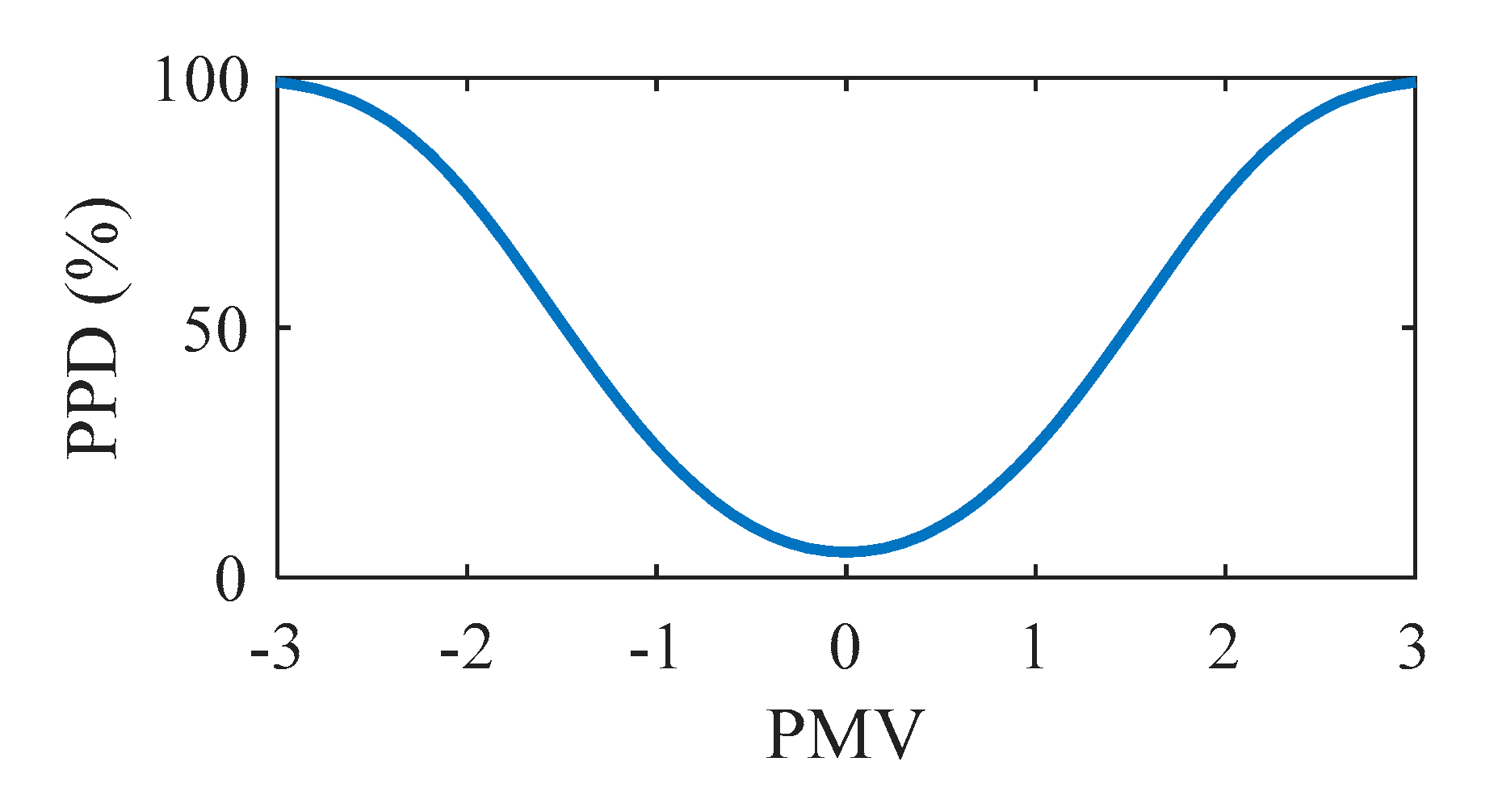
Fanger’s PMV model establishes a relationship between the thermal load on the body and the average thermal sensation of individuals. The thermal load on the body is expressed as a function of environmental factors (e.g., temperature, humidity, air velocity, and wall temperature) and individual factors (e.g., activity and clothing insulation). Based on the PMV, Fanger proposed a complementary index, called the predicted percentage of dissatisfied (PPD). The PPD represents the expected percentage of people who are thermally uncomfortable in an environment with a given PMV. The relationship between the PPD and the PMV is shown in Figure 5.

The present work is based on the PMV, in order to evaluate the passenger’s thermal comfort in a representative way. The HVAC system model allows calculating the cabin environment factors, whereas the individuals factors are given data (passengers at rest, type of clothing). When it helps interpreting the results, the PPD is also used. Results presented in Section 4 show that, in addition to the temperature and the humidity, the temperature of the cabin walls has a significant influence on thermal comfort, and hence on the HVAC control and consumption as well.

3.3. Phase 1: Traction Energy Estimation

The dynamic model of the powertrain, presented in Section 2, requires the knowledge of the exact speed profile in order to calculate the power required for a given trip. In real life at the beginning of the trip, this information is not available, but the navigation aid system can provide statistics about the speed along the planned route. Based on numerous simulations using the dynamic model, we have developed an estimator that predicts the average traction power as a function of the expected average vehicle speed $\overline{v}$, its standard deviation ${\sigma }_v$ and the road slope $p$. The estimated traction power ${\tilde{P}}_{traction}$ is postulated as the sum of a bicubic function of $\overline{v}$ and ${\sigma }_v$, and a term to account for the slope $p$, as given by (14), where $a_{i,j}$ and $b$ are coefficients to be identified, $m_{veh}$ is the mass vehicle and $g$ is the gravitational acceleration:

$${\tilde{P}}_{traction}\left(\overline{v},{\sigma }_v,p\right)={\displaystyle \sum }_{i=0}^3{\displaystyle \sum }_{j=0}^3{a}_{i,j}·{\overline{v}}^i·{\sigma }_v{}^j+b·m_{veh}·g·\sin \left({\tan }^{-1}\left(p\right)\right)$$

(14)

The coefficients of the model have been identified using 1200 speed cycles corresponding to various driving conditions [26]. Each speed cycle has been characterized by its mean value and standard deviation $\overline{v}$ and ${\sigma }_v$, and simulated by the powertrain model for different fixed slopes $p$, ranging from $-10\%$ to $+10\%$. This gives a total number of 168000 scenarios. Then, the average traction power over each cycle has been calculated, and linear regression has been used to compute the coefficients $a_{i,j}$ and $b$.

The accuracy of this estimation is assessed by analyzing the absolute and relative difference between ${\tilde{P}}_{traction}$, the average traction power estimated by (14), and $\overline{P_{traction}}$, the average traction power calculated by the dynamic powertrain model. These quantities, denoted respectively by $\mathsf{\Delta }{P}_{abs}$ and $\mathsf{\Delta }{P}_{rel}$, are defined by equations (15) and (16):

$$\mathsf{\Delta }{P}_{abs} \left[\mathrm{Wh}\right]=\left|{\tilde{P}}_{traction}-\overline{P_{traction}}\right|$$

(15)

$$\mathsf{\Delta }{P}_{rel} [\%]=\left|\frac{{\tilde{P}}_{traction}-\overline{P_{traction}}}{\overline{P_{traction}}}\right|$$

(16)

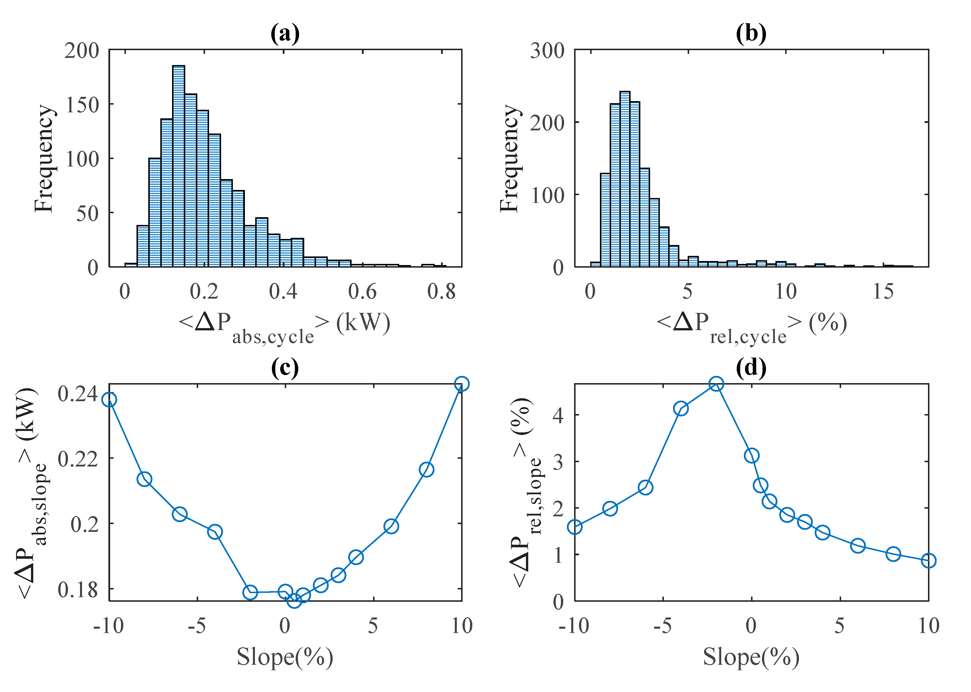
Figure 6 summarizes the estimator accuracy through different mean values of $\mathsf{\Delta }{P}_{abs}$ and $\mathsf{\Delta }{P}_{rel}$. The plots (a) and (b) show the histograms of $\langle \mathsf{\Delta }{P}_{abs,cycle}\rangle$ and $\langle \mathsf{\Delta }{P}_{rel,cycle}\rangle$, i.e., the mean value of $\mathsf{\Delta }{P}_{abs}$ and $\mathsf{\Delta }{P}_{rel}$, averaged over the slope for a given cycle. The errors mainly lie in the ranges $\left[0 \mathrm{W},300 \mathrm{W}\right]$ and $\left[0\%,5\%\right]$ respectively, with a mean value of $204 \mathrm{W}$ and $2.5\%$. Next, the curves (c) and (d) show the influence of the slope on $\langle \mathsf{\Delta }{P}_{abs,slope}\rangle$ and $\langle \mathsf{\Delta }{P}_{rel,slope}\rangle$, i.e., the mean value of $\mathsf{\Delta }{P}_{abs}$ and $\mathsf{\Delta }{P}_{rel}$, averaged over all the cycles, for a given slope. Although the absolute error increases with the slope, the relative error decreases because the traction power also increases with the slope (it reaches 100 kW for a 10% slope).

A second series of tests was performed using Institut National de Recherche sur les Transports et leur Sécurité (INRETS) and Laboratoire Central des Ponts et Chaussées (LCPC) (who merged in 2011 to create Institut Français des Sciences et Technologies des Transports, de l’Aménagement et des Réseaux – IFSTTAR) driving cycles, which were not used for the identification process. INRETS cycles are a set of ten driving cycles that have been built with data logged around Lyon (France), in various driving environments. The main characteristics of these cycles are reported in

Table 2. Characteristics of the UL1, UF1, R2 and A2 INRETS driving cycles.

INRETS Cycles	Duration [s]	Distance [km]	$\overline{\mathit{v}}$ [km/h]	${\mathit{\sigma }}_{\mathit{v}}$ [km/h]
UL1	806	0.85	3.81	4
UL2	812	1.67	7.42	6.22
UF1	681	1.88	9.92	9.74
UF2	1055	5.61	19.14	12.97
UF3	1068	7.23	24.36	16.43
R1	889	7.79	31.55	21.94

. Figure 7 shows four of these cycles (UL1, UF1, R2 and A2), representative of urban slow, urban fluid, road and highway traffic.

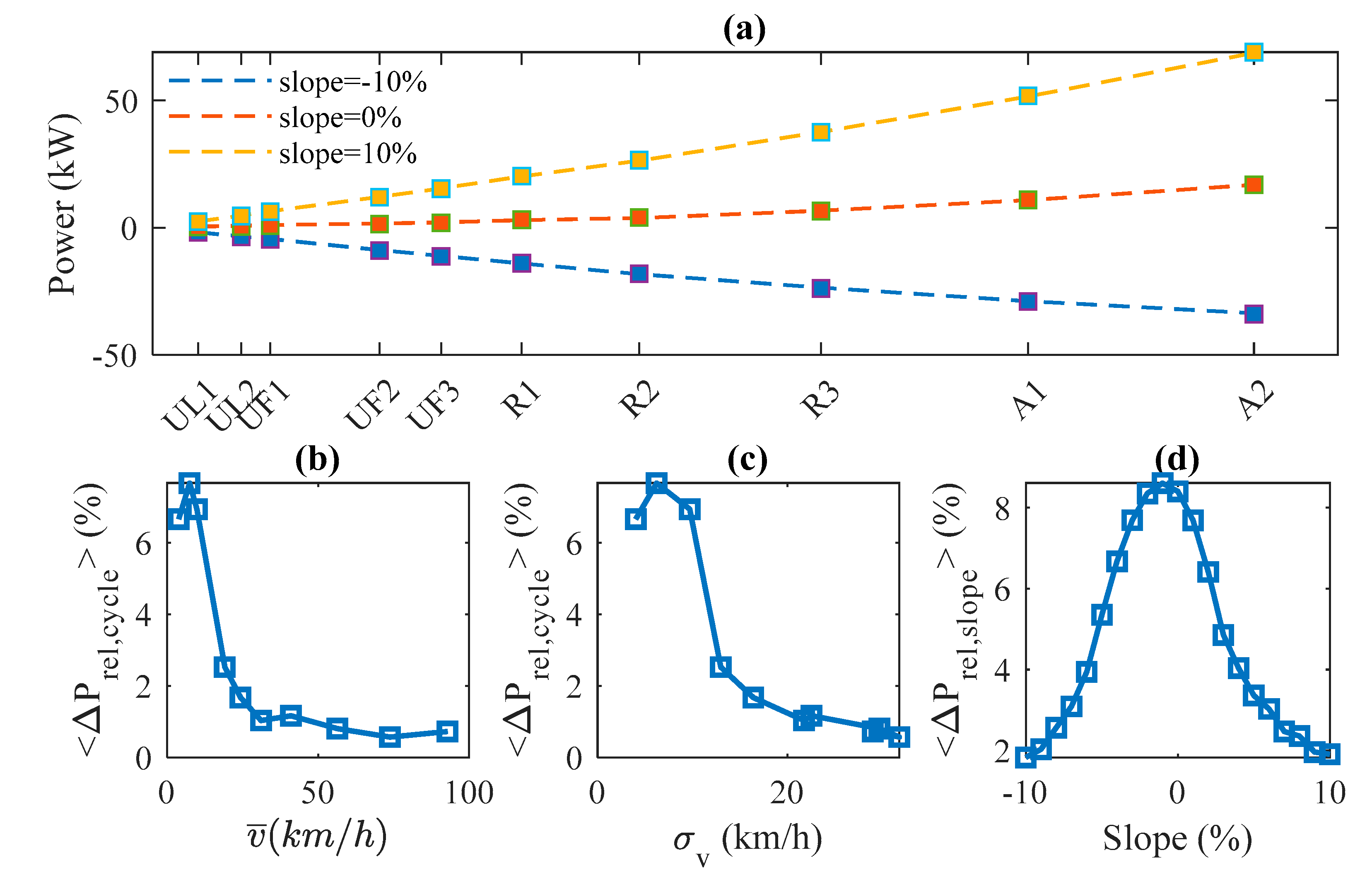
Figure 8 reports the results of the traction power estimator for the INRETS driving cycles. The plot (a) compares the estimated power ${\tilde{P}}_{traction}$ (dotted line) to $\overline{P_{traction}}$ (square), for different uniform slopes. The negative values, obtained for $p=-10\%$, reflect regenerative braking. The plots (b) and (c) show the average relative error for a given cycle $\langle \mathsf{\Delta }{P}_{rel,cycle}\rangle$ as a function of the speed average value $\overline{v}$ and the standard deviation ${\sigma }_v$, whereas the plot (d) shows the average relative error for a given slope $\langle \mathsf{\Delta }{P}_{rel,slope}\rangle$ as a function of the slope. The overall fit is good.

In real life conditions, the navigation aid system splits the planned route into a certain number of road sections of various length $l$ and provides the slope as well as traffic information for each of them. The total traction energy, ${\tilde{E}}_{traction}$, should then be computed by summing up the traction energy corresponding to each road sections according to Equation (17), where the subscript k refers to the kth section and $n$ denotes the number of sections:

$${\tilde{E}}_{traction}={\displaystyle \sum }_{k=1}^n{\tilde{E}}_{traction,k}={\displaystyle \sum }_{k=1}^n{\tilde{P}}_{traction}\left({\overline{v}}_k,{\sigma }_{v,k},p_k\right)\times \frac{l_k}{{\overline{v}}_k}$$

(17)

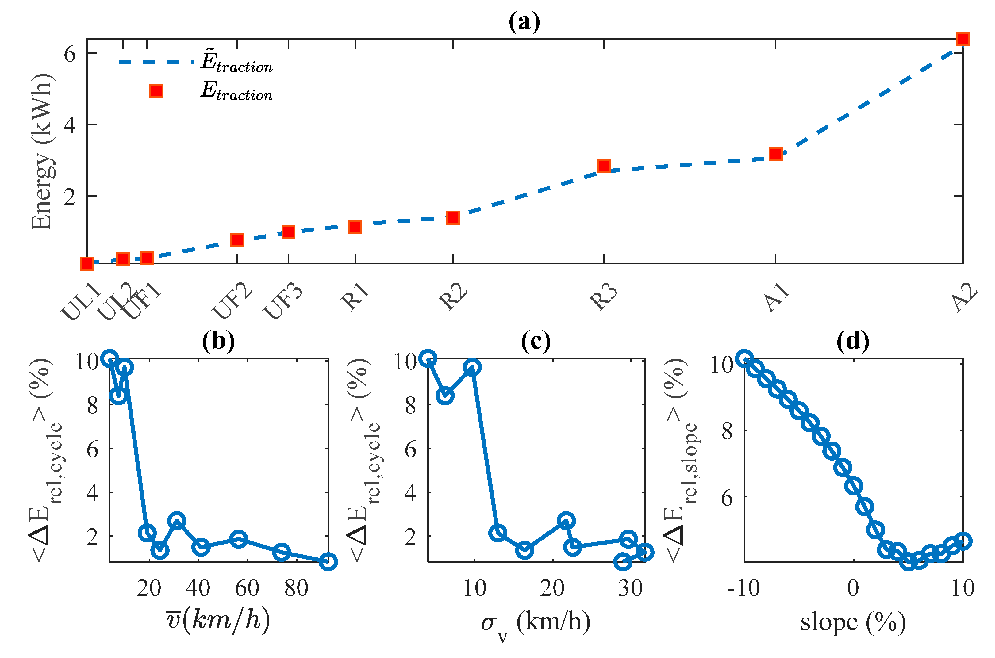
We have tested this technique by splitting the INRETS cycles into 500 m sections. Figure 9 shows the results. The plot (a) represents the energy calculated using the dynamic model (red squares) and estimated by splitting the road into $k$ road sections, according to equation (17), for $p=0\%$. The plots (b) and (c) show the average relative error for a given cycle $\langle \mathsf{\Delta }{E}_{rel,cycle}\rangle$ as a function of the average speed value $\overline{v}$ and the standard deviation ${\sigma }_v$, whereas the plot (d) shows the average relative error for a given slope, $\langle \mathsf{\Delta }{E}_{rel,slope}\rangle$, as a function of the slope. Again, the overall fit is good. The mean relative error $\langle \mathsf{\Delta }{E}_{rel,slope}\rangle$ is around $4.8\%$ for positive slopes but can reach $10\%$ for $p=-10\%$. We also notice that the mean relative error $\langle \mathsf{\Delta }{E}_{rel,cycle}\rangle$ decreases according to INRETS average speed and INRETS speed standard deviation.

3.4. Phase 2: Fast Cooling and HVAC Power Estimation

The fast cooling phase starts once the energy available for operating the air conditioning system, during the whole trip, is known. Its goal is to reach rapidly a thermal comfort that can be sustained until the end of the planned trip. The HVAC system is operated at its maximum cooling capacity, i.e., at maximum compressor rotational speed $N_{comp,max}$ and air flow rate ${\dot{m}}_{air,max}$. The heating system is disabled $\left({\alpha }_{min}=0\right)$ and the recycled air ratio is set at its maximum value ${\beta }_{max}=90\%$ (air quality issues require at least 10% air renewal).

The initial cabin temperature and humidity are assumed to be the same as outside (a vehicle parked in a shaded space). For the considered warm weather situations, they correspond to a large positive value of PMV. As soon as the control vector $u_{cooling}={\left[N_{comp,max},{\dot{m}}_{air,max},{\alpha }_{min},{\beta }_{max}\right]}^{\prime }$ is applied, the cabin temperature decreases while the thermal comfort starts to improve. All along the cooling phase, the TCMS monitors, in real time, the PMV. As it will be explained in the next paragraphs, it also estimates the amount of energy that the HVAC system would consume, if the thermal comfort was kept constant at its current value until the end of the trip. As long as this energy is less than the energy available for the HVAC system and that ideal comfort has been reached, the cooling phase goes on. The cooling phase stops when the system has reached a PMV that is either optimal ($PMV=0$) or that cannot be improved, given the energy available for the HVAC system.

The prediction of the energy, required to maintain the $PMV$ at a given value during the trip, is based on the use of a look-up table $G$, which gives an estimate of the optimal power consumed by the HVAC system for maintaining a desired PMV, denoted here by $PM{V}_{steady}$, in given conditions $w=\left[T_{ext},{\varphi }_{ext},P_{sun},v\right]$. This power is denoted by $P_{HVAC}{}^{*}\left(PM{V}_{steady},w\right)$ as formalized by Equation (18):

$$P_{HVAC}{}^{*}\left(PM{V}_{steady},w\right)=G\left(PM{V}_{steady},T_{ext},{\varphi }_{ext},P_{sun},v\right)$$

(18)

This look-up table is built off-line, based on simulation results under static conditions, as explained in Appendix A. It is used on-line, in real time dynamic conditions according to the following principle. The predicted environment conditions along the trip are denoted by $\tilde{w}\left(t\right)$. At time $t_k$ of the cooling phase, the current PMV index is $PMV\left(t_k\right)$. The estimation of the energy required by the HVAC system in order to maintain this thermal comfort until the end of the trip, denoted by ${\tilde{E}}_{HVAC,maintain}\left(t_k\right)$, is obtained by integrating the estimated HVAC power, as stated by Equation (19):

$${\tilde{E}}_{HVAC,maintain}\left(t_k\right)=\underset{t_k}{\overset{t_{end}}{{\displaystyle \int }}}{P}_{HVAC}^{*}\left(PMV\left(t_k\right),\tilde{w}\left(t\right)\right)·dt$$

(19)

During the cooling phase, the TCMS also monitors the energy consumed by the HVAC system since the beginning of the trip, denoted by $E_{HVAC,cool}\left(t_k\right)$, and the energy available for the rest of the trip, denoted by $E_{HVAC,available}\left(t_k\right)$:

$$E_{HVAC,available}\left(t_k\right)=E_{HVAC,available}\left(t_0\right)-E_{HVAC,cool}\left(t_k\right)$$

(20)

As long as ideal thermal comfort has not been reached (i.e., $PMV>0$) and there is enough energy available to improve the current thermal comfort (i.e., $E_{HVAC,available}\left(t_k\right)>E_{HVAC,maintain}\left(t_k\right)$), the cooling phase goes on. As soon as either ideal thermal comfort is reached or energy limitation is detected, the cooling stops and the phase 3 starts.

3.5. Phase 3: Thermal Comfort Maintaining

Let us denote by $PM{V}_{set}$ the value of PMV reached at the end of the phase 2. The phase 3 consists in maintaining the current $PMV$ at this setting value, at the lowest energy cost. At each time $t_k$, given the current external conditions $w\left(t_k\right)$, the TCMS algorithm (see Algorithm 1) determines the set of commands that lead to $PMV\left(t_{k+1}\right)=PM{V}_{set}$, and selects the one with the lowest energy cost.

Algorithm 1. The main points of the TCMS algorithm are summarized hereunder

Input: battery initial state-of-charge; traffic prediction ($\overline{v}$ and ${\sigma }_v$ for each section of the planned road); weather prediction $w\left(t\right)$ along the planned road

Phase 1: Initialization

Estimate the required energy for traction along the whole planned trip

Calculate the energy available for thermal comfort during the whole planned

trip Output: energy available for thermal comfort during the whole planned trip

Phase 2: Fast cooling

While (current PMV > 0)

Estimate $E_{HVAC,maintain}$, the energy to maintain the current thermal comfort until the end of the trip

Calculate $E_{HVAC,available}$, the energy left for the thermal comfort until the end of the trip

If ($E_{HVAC,available}>E_{HVAC,maintain}$):

Apply maximum cooling command $u_{max}$

Else:

$PM{V}_{set}=current PMV$

Exit while loop

Output: Thermal comfort setting point for phase 3 $PM{V}_{set}$

Phase 3: Thermal comfort maintaining

For the rest of the trip:

Apply command $u$ such that $PMV=PM{V}_{set}$ at the lowest energy cost

Output: Predicted and actual HVAC power profile, PMV profile

4. Results and Discussion

The proposed real-time comfort management algorithm has been implemented and applied to the system model, in the MATLAB^® environment. Extensive simulations were run for a large number of scenarios with different weather conditions, traffics, and initial battery’s state-of-charge. This section presents the results and a statistical analysis is conducted in order to assess the capacity of the proposed method in adjusting the thermal comfort according to the amount of energy available for the HVAC system.

Firstly, we verify that the HVAC system consumption estimated during the cooling phase using the look-up table $G$ corresponds to its actual consumption, calculated afterwards using the system dynamic model. A good match justifies the relevance of using a precalculated static model in slowly varying conditions.

The next point is to evaluate the performance of the thermal comfort management algorithm. For this purpose, we formulate an optimization problem that consists into minimizing the global thermal comfort defined by (21) for a given amount of energy. Solving this problem using the dynamic programming approach presented in [20] provides reference solutions against which the real-time algorithm efficiency can be assessed:

$$J\left(u\right)=\underset{0}{\overset{t_{fin}}{{\displaystyle \int }}}PM{V}^2\left(x\left(u\left(t\right),w\left(t\right)\right)\right)dt$$

(21)

4.1. Test Scenarios

Each scenario corresponds to a one-hour trip completed in given weather and traffic conditions, with a certain initial battery’s state-of-charge. Regarding weather conditions, we have defined a scenario in which the solar radiation is constant, while the external temperature and humidity evolve, according to parametrized time profiles. The temperature profile $T_{ext}\left(t\right)$ is shown in Figure 10. The temperature rises from $T_{ext,0}$ at the beginning of the trip to $T_{ext,0}$ + 2 °C at halfway, and then decreases back to $T_{ext,0}$. As for the humidity, weather conditions are described in terms of relative humidity $RH$, whereas the thermodynamic equation is written using the specific humidity $\varphi$. The relationship between these two quantities is given by (22), where $P_{atm}$ is the atmospheric pressure and $P_{sat}$ denotes the saturated vapor pressure of water at the considered temperature:

$$R{H}_{ext}\left(t\right)=\frac{P_{atm}\times {\varphi }_{ext}\left(t\right)}{P_{sat}\left(T_{ext}\left(t\right)\right)\times \left({\varphi }_{ext}\left(t\right)+0.622\right)}$$

(22)

The chosen scenario assumes a linear increase of the specific humidity over the whole trip, from ${\varphi }_{ext,0}$ to ${\varphi }_{ext,0}+0.05$, where ${\varphi }_{ext,0}$ is calculated according to the values of the initial relative humidity $R{H}_{ext,0}$ and temperature $T_{ext,0}$. Figure 10 shows an example of the time evolution of the temperature, relative humidity and solar power for a weather scenario given the following parameters: $T_{ext,0}$ = 37 °C, $R{H}_{ext,0}=35\%$ and ${\dot{q}}_{sun,0}$ = 500 W.

Different values of the parameters $T_{ext,0}$, $R{H}_{ext,0}$, and ${\dot{q}}_{sun,0}$ correspond to different weather conditions. In order to explore a wide range of weather conditions, without focusing on the weather profile itself, we have combined together the following values: $T_{ext,0}\left[{}^{°}\mathrm{C}\right]\in \left\{25;26;\dots ;38\right\}$, $R{H}_{ext,0}\in \left\{0.35;0.45;0.55;0.65;0.75\right\}$, ${\dot{q}}_{sun,0}\left[\mathrm{W}/{\mathrm{m}}^2\right]\in \left\{0;500;1000\right\}$. This results in a total number of 210 weather scenarios. As the HVAC system efficiency depends on the vehicle speed, four traffic conditions, representative of congested urban, fluid urban, road and highway environments are modeled, using the UL1, UF1, R2 and A2 INRETS driving cycles (Figure 7). Each type of cycle is repeated several times in order to construct a 1 h speed profiles, corresponding to the following distances: 4.25, 11.28, 46.3 and 105.92 km, respectively. In addition, a variable slope is considered.

The initial temperature and relative humidity in the cabin are assumed the same as outside (vehicle parked in a shaded space). For all the tested scenarios, we consider that passengers are seated and lightly dressed, (i.e., a shirt, underpants, trousers, socks and shoes), which corresponds to a clothing insulation of 1.1 clo $\left(0.155 {\mathrm{m}}^2\mathrm{K}/\mathrm{W}\right)$ (see Nilsson’s thesis [27]). The uncertainty on this value is estimated to be ±0.1 clo according to [28]. In [29], the driving activity is estimated to correspond to 1.4 met, while in ASHRAE standard [23], a broader range is suggested, from 1 met to 2 met. Since the physical activity in an electric vehicle is lower than the activity in a conventional one (no clutching, shifting gears, … etc.), the metabolism rate may be lower than 1.4. We assume therefore that driving corresponds to a metabolism rate of 1 met (58.2 W/m²), with an uncertainty of +0.2 met. Finally, the air speed in the cabin is assumed to be equal to 1 m/s.

Five initial SOC of the battery are tested, each one corresponds to a given amount of energy available for thermal comfort.

In summary, the benchmark built from the abovementioned scenarios corresponds to four given trips, which are carried out in 210 weather conditions, with five different levels of available energy. The total number of test cases reaches 4200. A summary of simulation data is reported in

Table 3. Summary of test case data.

Data	Values
External temperature	$T_{ext,0}\left[{}^{°}\mathrm{C}\right]\in \left\{25;26;\dots ;38\right\}$
External relative humidity	$R{H}_{ext,0}\in \left\{0.35;0.45;0.55;0.65;0.75\right\}$
Solar radiation	${\dot{q}}_{sun,0}\left[\mathrm{W}/{\mathrm{m}}^2\right]\in \left\{0;500;1000\right\}$
Average speed	Extracted from INRETS driving cycles: A2, R2, UF1 & UL1
Speed standard deviation
Slope	Variable slope profile
Clothing insulation	1.1 clo
Metabolism	1 met
Air speed	1 m/s

. This large number of situations allows assessing the capacity of the proposed real-time algorithm in adjusting the thermal comfort according to the available energy.

The real-time thermal comfort management algorithm has been applied to the system model for each of the 4200 scenarios. The results are presented hereafter.

4.2. Ideal Comfort Results

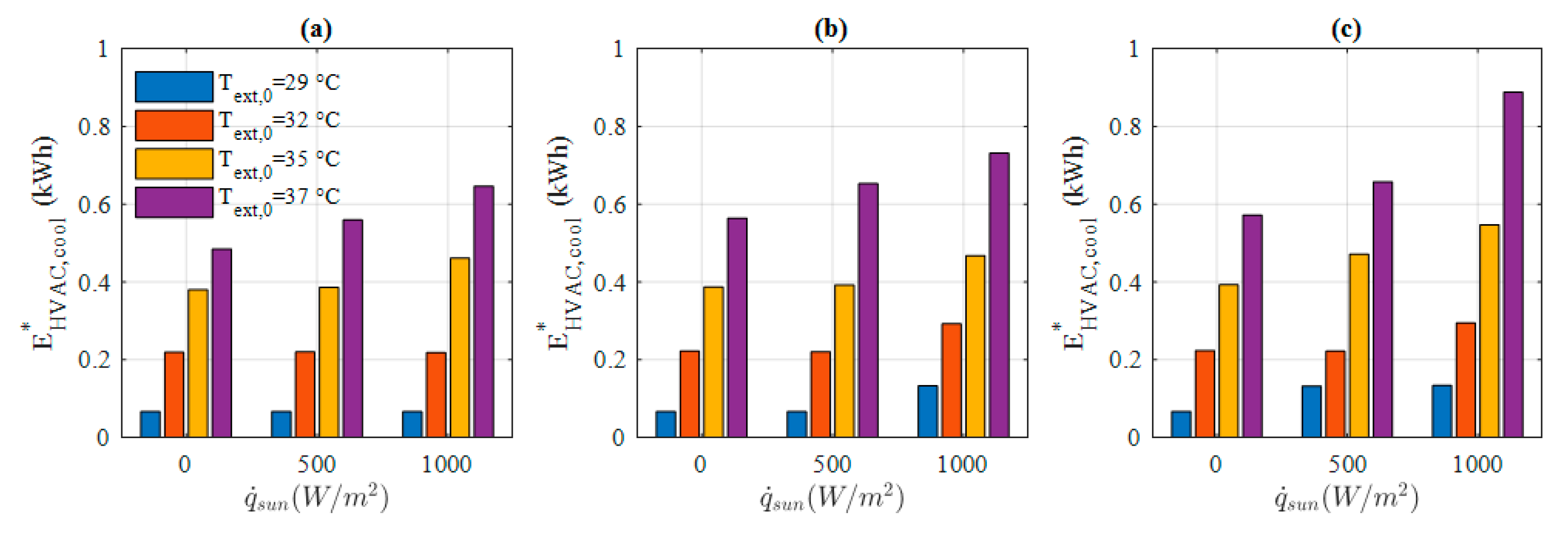
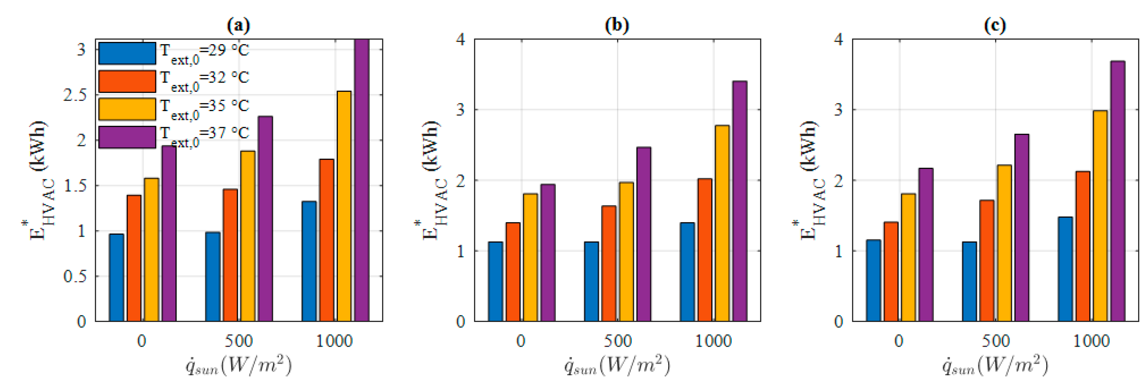
This section reports some observations and analysis on three physical quantities, corresponding to ideal comfort conditions: (i) the HVAC system consumption, $E_{HVAC}^{*}$ needed for ideal comfort, (ii) the cooling energy $E_{HVAC,cool}^{*}$ consumed to reach the ideal comfort value PMV = 0 (cooling phase), (iii) the ratio $r_{HVAC}^{*}$ between $E_{HVAC}^{*}$ and the total energy (sum of $E_{HVAC}^{*}$ and traction energy), (iv) the steady state cabin temperature $T_{cab,steady}$. Figure 11 and Figure 12 summarize obtained results related to $E_{HVAC}^{*}$ and $E_{HVAC,cool}^{*}$ for a driver dressed lightly, in a suburban traffic (i.e., INRETS R2 driving cycle). The graphs show the evolution of $E_{HVAC}^{*}$ and $E_{HVAC,cool}^{*}$ as a function of solar radiation for different values of $T_{ext,0}$ and $R{H}_{ext,0}$. We observe that both $E_{HVAC}^{*}$ and $E_{HVAC,cool}^{*}$ are increasing functions of the solar radiation, outside temperature and relative humidity. For instance, for a typical hot summer day (i.e., $T_{ext,0}$ = 32 °C, $R{H}_{ext,0}=55\%$, ${\dot{q}}_{sun}$ = 1000 W/m²), $E_{HVAC}^{*}$ and $E_{HVAC,cool}^{*}$ reach respectively 2 kWh and 0.3 kWh.

Figure 13 summarizes the results of $r_{HVAC}^{*}$ for a moderate humid weather (i.e., $R{H}_{ext,0}=55\%$). The graphs show the values of $r_{HVAC}^{*}$ corresponding to four driving cycles: INRETS A2, R2, UF1 and UL1, for different $T_{ext,0}$ and ${\dot{q}}_{sun,0}$. The results illustrate the relative high value of $r_{HVAC}^{*}$ in congested and fluid urban conditions. This is mainly due to the low traction energy at low speed. For instance, for a typical hot summer day, in congested urban condition, this ratio reaches 84.5%. Results also show that for the same driving cycle, this ratio increases with outside temperature and solar radiation.

It is worth underlining the capacity of the PMV model to account for the cabin wall temperature. As an illustrative example, we have simulated an ideal thermal comfort ($PMV=0$) for given external temperature and humidity ($T_{ext}$ = 37 °C, $R{H}_{ext}=35\%$) but with different solar radiation levels ${\dot{q}}_{sun,0}$ ($0$, $500$ and $1000$ W/m²).

Table 4. Cabin temperature, wall temperature and consumed energy for ideal comfort (PMV = 0) for different solar radiations.

${\mathit{P}}_{\mathit{s}\mathit{u}\mathit{n}}$ [W/m2]	${\mathit{T}}_{\mathit{w}\mathit{a}\mathit{l}\mathit{l}}$ [°C]	${\mathit{T}}_{\mathit{c}\mathit{a}\mathit{b}}$ [°C]	${\mathit{E}}_{\mathit{H}\mathit{V}\mathit{A}\mathit{C}}$ [kWh]
0	25.1	24.7	1.94
500	31.3	23	2.26
1000	37.3	21.2	3.12

reports the corresponding cabin wall temperature $T_{wall}$, cabin ambiant temperature $T_{cab}$, and HVAC system energy consumption for the same trip. In the absence of solar radiation (at night), $T_{wall}$ = 25.1 °C, and ideal thermal comfort is obtained for $T_{cab}$ = 24.7 °C. In sunny conditions, other parameters being equal, $T_{wall}$ = 37.3 °C, and ideal comfort requires a cooler ambiant temperature, $T_{cab}$ = 21.2 °C, and more energy.

4.3. Qualitative Observations for a Specific Scenario

The present section summarizes some qualitative observations made for a particular scenario, defined by $T_{ext,0}$ = 37 °C, $R{H}_{ext,0}=35\%$, ${\dot{q}}_{sun,0}$ = 500 W (Figure 10) and the R2 driving cycle. Similar trends are observed for all other scenarios

Figure 14 shows the temporal evolution of the PMV, the temperature and the relative humidity in the cabin, for three initial battery state–of-charge. The PMV profile has the desired shape: it drops at the beginning of the trip, and then keeps constant at a PMV level that depends on the available energy. For an initial SOC of 29.2 %, the embedded energy is sufficient for almost reaching the ideal thermal comfort after a 9-min cooling phase ($PMV=0.06$).

For an initial SOC of 28%, the cooling phase stops earlier, at a PMV of 1, which remains acceptable for passengers. For an initial SOC of 26.6 %, the cooling phase is even shorter and the PMV is 1.8. Figure 14b,c display the corresponding temperature and humidity in the cabin. It is worth noting that both quantities evolve over time despite a constant value of PMV index, reflecting the fact that a given PMV can be obtained with different combinations of temperature and humidity.

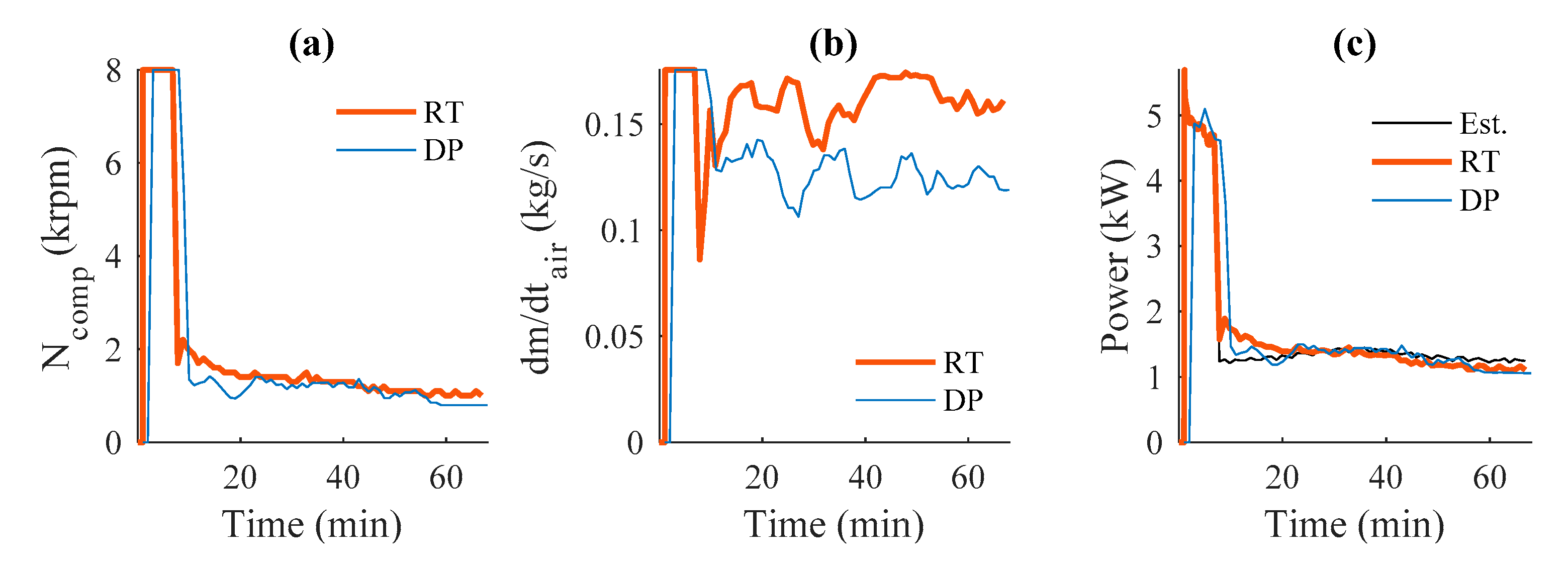
Figure 15 focuses on the particular scenario with an initial SOC of 28%. The red curves correspond to the results obtained by TCMS, whereas the blue curves represent results obtained by dynamic programing [21], which serve as a reference. Two of the four HVAC control variables are plotted versus time, the compressor rotation speed (Figure 15a) and the air flow (Figure 15b). These commands are set at their maximum value during the cooling phase, and then adjusted in order to maintain the target PMV at the lowest energy cost. One notices that, despite the temporal variations of the weather conditions, the control variables do not significantly change. Small oscillations reflect the search process of the control vector, which consists in minimizing the air conditioning power at all time. During the process, very close air conditioning powers are achieved with different combinations of $N_{comp}$, ${\dot{m}}_{air}$, $\alpha$ and $\beta$. Since the algorithm selects the combination that minimizes the HVAC power, the values of ${\dot{m}}_{air}$ can naturally differ from one step to the next. Figure 15c reports the HVAC system power estimated during the cooling phase using the look-up table (black line), actually consumed during the trip (red line). Both curves are very close to one another, indicating a good quality of the power prediction using the look-up table $G$.

4.4. Statistical Analysis over All the Scenarios

The present section reports the analysis of the results over a wide range of scenarios, necessary in order to assess the proposed real-time approach. Two aspects ought to be evaluated through relevant performance metrics, the power estimation accuracy on one hand, and the efficiency of the thermal comfort management on the other hand.

Firstly, the adequacy of using the static mapping $G$ in a dynamic context is quantified by looking at the absolute and relative differences between the HVAC energy estimated at the end of cooling phase, denoted by $E_{estimated}$, and the energy actually consumed during the trip, denoted by $E_{actual}$. The two metrics $\mathsf{\Delta }{E}_{abs}$ and $\mathsf{\Delta }{E}_{rel}$ are defined by equations (23) and (24):

$$\mathsf{\Delta }{E}_{abs}=E_{actual}-E_{estimated}$$

(23)

$$\mathsf{\Delta }{E}_{rel}=\frac{E_{actual}-E_{estimated}}{E_{actual}}$$

(24)

Figure 16a,b represent the histograms of $\mathsf{\Delta }{E}_{abs}$ and $\mathsf{\Delta }{E}_{rel}$ calculated for each of the 1050 scenarios run for the driving cycle INRETS R2.

Table 5. Mean value and standard deviation of $\mathsf{\Delta }{E}_{abs}$ and $\mathsf{\Delta }{E}_{rel}$ for the four tested driving cycles.

INRETS Cycles	$$\mathsf{\Delta }{\mathit{E}}_{\mathit{a}\mathit{b}\mathit{s},\mathit{m}\mathit{e}\mathit{a}\mathit{n}}$$ [Wh]	$$\mathsf{\Delta }{\mathit{E}}_{\mathit{a}\mathit{b}\mathit{s}, \mathit{s}\mathit{t}\mathit{d}}$$ [Wh]	$$\mathsf{\Delta }{\mathit{E}}_{\mathit{r}\mathit{e}\mathit{l},\mathit{m}\mathit{e}\mathit{a}\mathit{n}}$$ [%]	$$\mathsf{\Delta }{\mathit{E}}_{\mathit{r}\mathit{e}\mathit{l},\mathit{s}\mathit{t}\mathit{d}}$$ [%]
A2	−14.3	48.8	−1.7	3.4
R2	−40.7	55.9	−3.8	4.2
UF1	−32.5	55.3	−3.2	4
UL1	−4.9	67.8	−1.6	4.5

reports the mean value (subscript $mean$) and the standard deviation (subscript $std$) of $\mathsf{\Delta }{E}_{abs}$ and $\mathsf{\Delta }{E}_{rel}$ for each of the four tested driving cycles. These metrics show that the estimation, based on the look-up table G, is quite reasonable and can be trusted.

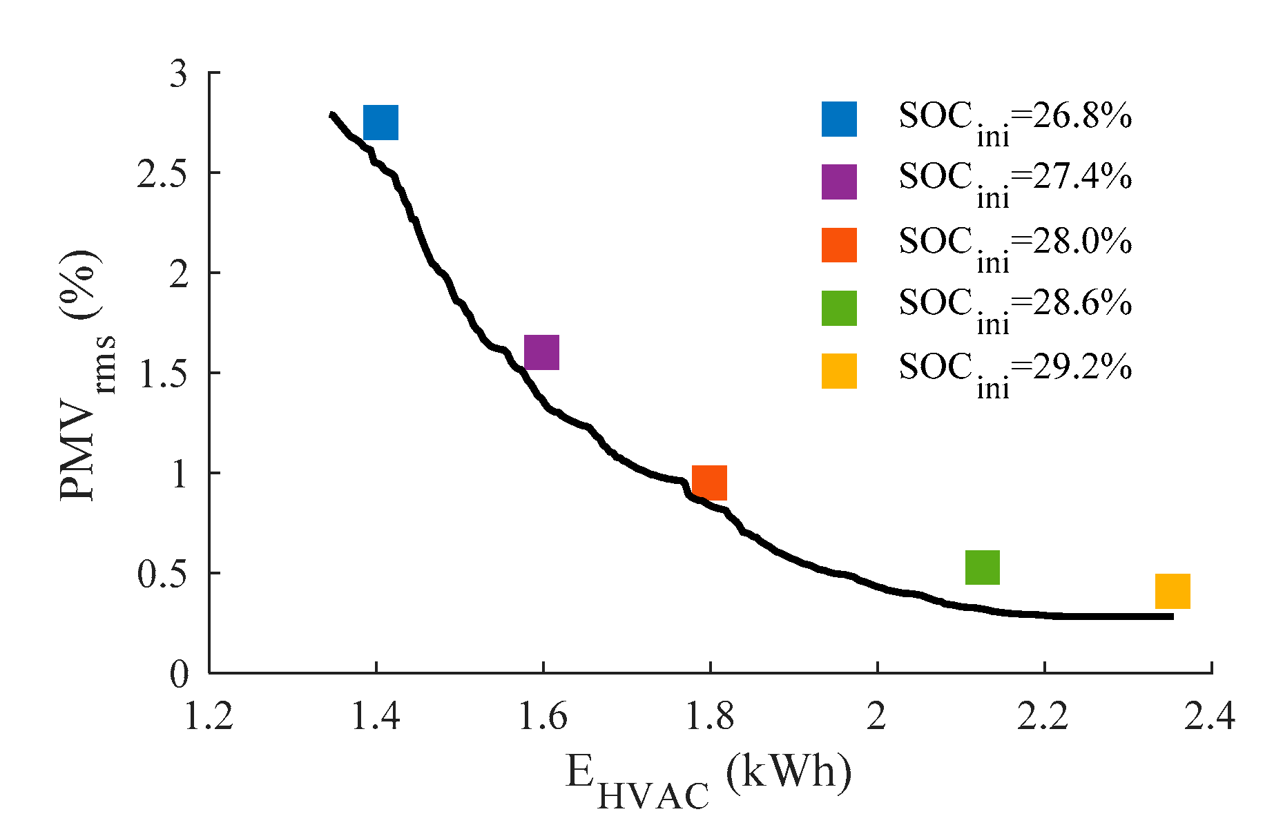
The comparison between the results of our real-time strategy and the optimal ones given by dynamic programming needs to account for two criteria, the total energy consumed by the HVAC system and the root mean square of the PMV, respectively denoted by $E_{HVAC}$ and $PM{V}_{rms}$. The different solutions obtained for a given weather and traffic scenario are reported in the $\left(E_{HVAC},PM{V}_{rms}\right)$ plane. Figure 17 shows the results for the scenario defined by $T_{ext,0}$ = 37 °C, $R{H}_{ext,0}=35\%$, ${\dot{q}}_{sun,0}$ = 500 W and the R2 driving cycle. The black line corresponds to dynamic programming results and constitutes the Pareto frontier of the $\left(E_{HVAC},PM{V}_{rms}\right)$ bicriteria optimization problem. The colored points correspond to the proposed real-time control algorithm. As expected, they lie above the Pareto frontier, but at a small distance, indicating that the proposed algorithm gives near-optimal results for this particular scenario.

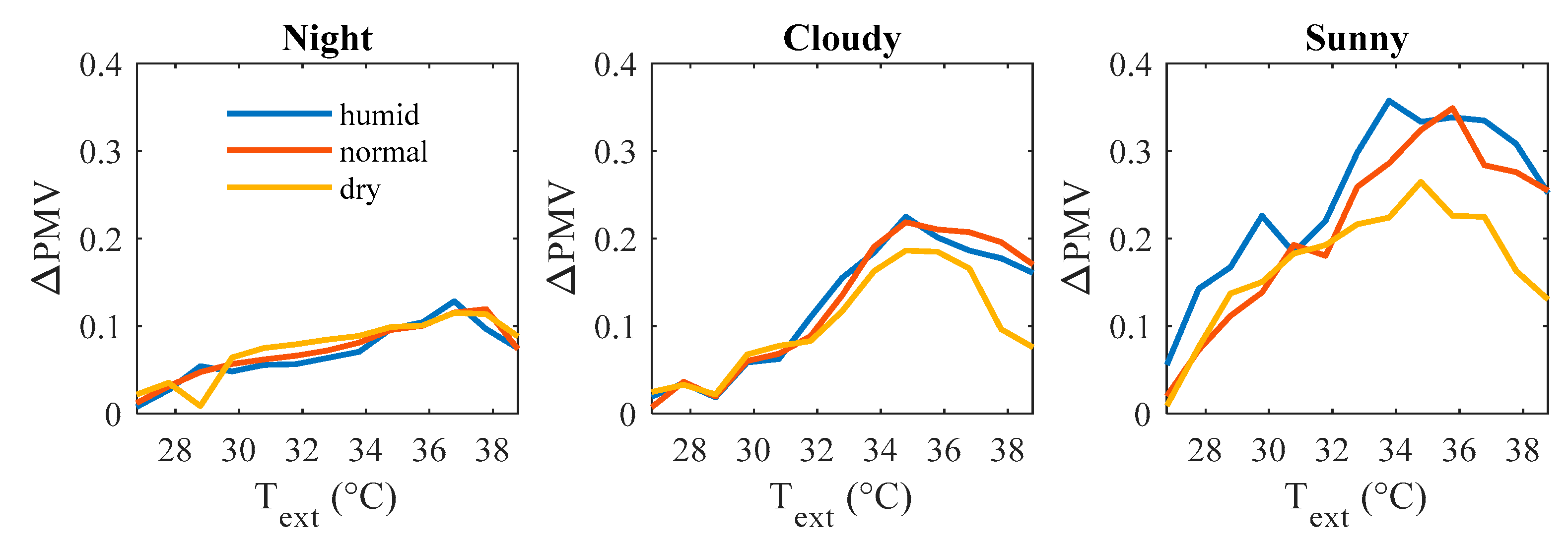
We have chosen to quantify the performance of the proposed TCMS by the average vertical distance between the colored points and the Pareto frontier. This distance is denoted by $\mathsf{\Delta }PM{V}_{DP}$. The smaller it is, the better the real-time algorithm performs.

Figure 18 summarizes the results for the R2 driving cycles. The curves show the evolution of $\mathsf{\Delta }PM{V}_{DP}$, as a function of the external temperature, for different conditions of humidity and insolation. The average value is $0.15$, and we notice that this difference increases in warm and sunny conditions. Similar results are obtained for the other driving cycles, but we prefer not to present them here since they show same behavior.

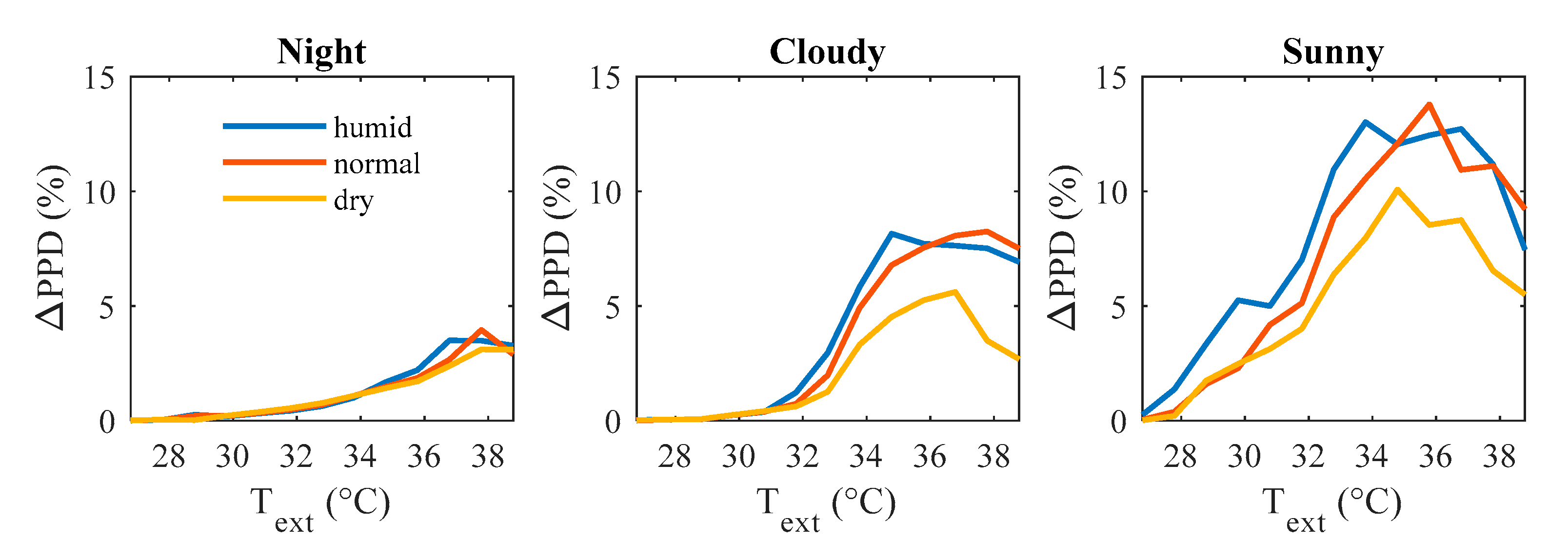
The performance of the TCMS can also be assessed using the PPD index for a given PMV [22]. This criterion has the advantage of being less abstract than the PMV. In a similar way than $\mathsf{\Delta }PM{V}_{DP}$, we define the metrics $\mathsf{\Delta }PP{D}_{DP}$ as the average difference between the root mean square value of the PPD obtained with the real-time algorithm, and the root mean square value of the PPD obtained by dynamic programming for the same HVAC energy. Figure 19 shows the $\mathsf{\Delta }PM{V}_{DP}$ evolution as a function of temperature, for given humidity and isolation conditions. The average $\mathsf{\Delta }PP{D}_{DP}$ value is equal to $3\%$.

5. Conclusions and Perspectives

This paper presented a real time management approach of thermal comfort in EVs for given traffic and weather predictions provided by the navigation aid system. For this purpose, a realistic model of the HVAC system and a representative thermal comfort index were used.

Two estimators were built. The first one estimates the traction power in given traffic conditions, which we propose to model by the average value and standard deviation of the speed. This estimator is used to calculate the traction energy necessary to complete the trip. Validation tests were run to assess its accuracy, for different driving cycles and slopes. Results showed that the average estimation error is about 3%.

The second estimator was needed to estimate the HVAC system power consumption for a given thermal comfort level, in given meteorological and speed conditions. It was built off-line and used on-line by the TCMS, the proposed real-time algorithm, in order to adapt the thermal comfort level according to the energy available for the coming trip. In order to prove its validity, simulations were conducted for different traffic and weather conditions scenarios, and different initial battery SOCs. Results showed a good fit between the estimated and actual consumption.

The same scenarios were used to assess the near optimality of the overall approach, by comparing it to an optimal control approach. Results showed that for the same consumed energy, the real-time algorithm increased the discomfort by only 3%.

In its current version, the TCMS does not update the predictions during the trip, but further development is in progress to include this important aspect of real-time control. For example, traffic changes will affect the energy available for the HVAC system, and consequently require to periodically updating the thermal comfort level target, according to the latest predictions. Other tests will be conducted for changing driving predictions and several weather scenarios.

Other perspectives could include thermal comfort management for more than one occupant. Also, two or three zone HVAC operation can be considered for better thermal comfort evaluation accuracy. Finally, a fast cooling phase with two stages: opening windows and then operating the HVAC system, may be an interesting solution to reduce further the consumption.

References

1. Ibrahim, B.S.K.K.; Aziah, M.A.N.; Ahmad, S.; Akmeliawati, R.; Nizam, H.M.I.; Muthalif, A.G.A.; Toha, S.F.; Hassan, M.K. Fuzzy-based Temperature and Humidity Control for HV AC of Electric Vehicle. Procedia Eng. 2012, 41, 904–910. [Google Scholar] [CrossRef] [Green Version]
2. Beinarts, I. Fuzzy logic control method of HVAC equipment for optimization of passengers’ thermal comfort in public electric transport vehicles. In Proceedings of the Eurocon 2013, Zagreb, Croatia, 1–4 July 2013; pp. 1180–1186. [Google Scholar]
3. Fayaz, M.; Ullah, I.; Shah, A.S.; Kim, D. An Efficient Energy Consumption and User Comfort Maximization Methodology Based on Learning to Optimization and Learning to Control Algorithms. J. Intell. Fuzzy Syst. 2019, 37, 6683–6706. [Google Scholar] [CrossRef]
4. Xie, Y.; Liu, Z.; Liu, J.; Li, K.; Zhang, Y.; Wu, C.; Wang, P.; Wang, X. A Self-learning intelligent passenger vehicle comfort cooling system control strategy. Appl. Therm. Eng. 2020, 166, 114646. [Google Scholar] [CrossRef]
5. Sakhdari, B.; Azad, N.L. An Optimal Energy Management System for Battery Electric Vehicles. IFAC-PapersOnLine 2015, 48, 86–92. [Google Scholar] [CrossRef]
6. Mansour, C.; Nader, W.B.; Breque, F.; Haddad, M.; Nemer, M. Assessing additional fuel consumption from cabin thermal comfort and auxiliary needs on the worldwide harmonized light vehicles test cycle. Transp. Res. Part D Transp. Environ. 2018, 62, 139–151. [Google Scholar] [CrossRef]
7. Shojaei, S. Application of Key-off Cooling and Partial Charging in Plug-in Electric Vehicles; Phd thesis. University of Warwick: Coventry, UK, 2018. [Google Scholar]
8. de Nunzio, G.; Sciarretta, A.; Steiner, A.; Mladek, A. Thermal management optimization of a heat-pump-based HVAC system for cabin conditioning in electric vehicles. In Proceedings of the 2018 Thirteenth International Conference on Ecological Vehicles and Renewable Energies (EVER), Monte-Carlo, Monaco, 10–12 April 2018; pp. 1–7. [Google Scholar]
9. Hongwen, H.; Chen, W.; Hui, J. A Stochastic Model Predictive Controller Based on Combined Conditions of Air Conditioning System for Electric Vehicles. DEStech Trans. Environ. Energy Earth Sci. 2019. [Google Scholar] [CrossRef]
10. He, H.; Jia, H.; Sun, C.; Sun, F. Stochastic Model Predictive Control of Air Conditioning System for Electric Vehicles: Sensitivity Study, Comparison, and Improvement. IEEE Trans. Ind. Inform. 2018, 14, 4179–4189, No. 9. [Google Scholar] [CrossRef]
11. Vatanparvar, K.; Al Faruque, M.A. Design and Analysis of Battery-Aware Automotive Climate Control for Electric Vehicles. ACM Trans. Embed. Comput. Syst. 2018, 17, 22. [Google Scholar] [CrossRef]
12. Vatanparvar, K.; Al Faruque, M.A. Battery lifetime-aware automotive climate control for Electric Vehicles. In Proceedings of the 2015 52nd ACM/EDAC/IEEE Design Automation Conference (DAC), San Francisco, CA, USA, 8–12 June 2015; pp. 1–6. [Google Scholar]
13. Busl, M. Design of an Energy-Efficient Climate Control Algorithm for Electric Cars. Master’s Thesis, Lund University, Lund, Sweden, 2011. [Google Scholar]
14. Vatanparvar, K.; Al Faruque, M.A. Eco-Friendly Automotive Climate Control and Navigation System for Electric Vehicles. In Proceedings of the 2016 ACM/IEEE 7th International Conference on Cyber-Physical Systems (ICCPS), Vienna, Austria, 11–14 April 2016; pp. 1–10. [Google Scholar]
15. Vatanparvar, K.; Faezi, S.; Burago, I.; Levorato, M.; Al Faruque, M.A. Extended Range Electric Vehicle With Driving Behavior Estimation in Energy Management. IEEE Trans. Smart Grid 2019, 10, 2959–2968. [Google Scholar] [CrossRef]
16. Schaut, S.; Sawodny, O. Thermal Management for the Cabin of a Battery Electric Vehicle Considering Passengers’ Comfort. IEEE Trans. Control Syst. Technol. 2020, 28, 1476–1492. [Google Scholar] [CrossRef]
17. Bächle, T.; Graichen, K.; Buchholz, M.; Dietmayer, K. Model Predictive Heating Control for Electric Vehicles Using Load Prediction and Switched Actuators. IFAC-PapersOnLine 2016, 49, 406–411. [Google Scholar]
18. Esqueda-Merino, D.; Dubray-Demol, A.; Olaru, S.; Godoy, E.; Dumur, D. Energetic optimization of automotive thermal systems using mixed-integer programming and model predictive control. In Proceedings of the 2013 IEEE International Conference on Control Applications (CCA), Hyderabad, India, 28–30 August 2013; pp. 223–228. [Google Scholar]
19. He, H.; Jia, H.; Huo, W.; Yan, M. Stochastic Dynamic Programming of Air Conditioning System for Electric Vehicles. Energy Procedia 2017, 105, 2518–2524. [Google Scholar] [CrossRef]
20. Lahlou, A.; Ossart, F.; Boudard, E.; Roy, F.; Bakhouya, M. A dynamic programming approach for thermal comfort control in electric vehicles. In Proceedings of the IEEE Vehicle Power Propulsion Conf., Chicago, IL, USA, 27–30 August 2018. [Google Scholar]
21. Bellman, R. Dynamic Programming, 1st ed.; Princeton Univ. Press: Princeton, Princeton, USA, 1957. [Google Scholar]
22. Fanger, P.O. Thermal Comfort: Analysis and Applications in Environmental Engineering; McGraw-Hill: New York, NY, USA, 1970. [Google Scholar]
23. ANSI/ASHRAE Standard 55. Thermal Environmental Conditions for Human Occupancy; American Society of Heating, Refrigerating and Air conditioning Engineers: Atlanta, GA, USA, 1992. [Google Scholar]
24. Zhang, H.; Cao, D.; Du, H. Modeling, Dynamics, and Control of Electrified Vehicles; Woodhead Publishing: Cambridge, UK, 2017. [Google Scholar]
25. S.M. Mousavi, G.; Nikdel, M. Various battery models for various simulation studies and applications. Renew. Sustain. Energy Rev. 2014, 32, 477–485. [Google Scholar] [CrossRef]
26. Drive Cycle Data. Available online: https://www.nrel.gov/transportation/secure-transportation-data/tsdc-drive-cycle-data.htmlISO7730:2005(en) (accessed on 31 July 2019).
27. Nilsson, H. Comfort Climate Evaluation with Thermal Manikin Methods and Computer Simulation Models. Ph.D. Thesis, Royal Institute of Technology, Stockholm, Sweden, 2004. [Google Scholar]
28. Lee, J.H.; Kim, Y.K.; Kim, K.S.; Kim, S. Estimating Clothing Thermal Insulation Using an Infrared Camera. Sensors 2016, 16, 341. [Google Scholar] [CrossRef] [PubMed] [Green Version]
29. Metabolic Rate. Available online: https://www.engineeringtoolbox.com/met-metabolic-rate-d_733.html (accessed on 31 July 2020).
30. International Organization for Standardization (2005) Ergonomics of the Thermal Environment—Analytical Determination and Interpretation of Thermal Comfort using Calculation of the PMV and PPD Indices and Local Thermal Comfort Criteria (ISO 7730).
Figure 1. Schematic diagram of the HVAC system.
Energies 13 04006 g001
Figure 2. Schematic diagram of the air cooling and heating system: (a) compressor—(b) condenser—(c) expansion valve—(d) evaporator—(e) moto-ventilator group (MVG)—(f) ventilation fan. The points 1, 2, 5 & 6 correspond to different thermodynamic states of the refrigerant explained in Figure 3.
Energies 13 04006 g002
Figure 3. Refrigerating thermodynamic loop.
Energies 13 04006 g003
Figure 4. Schematic view of the proposed thermal comfort management strategy.
Energies 13 04006 g004
Figure 5. Relationship between the PMV and the PPD.
Energies 13 04006 g005
Figure 6. Assessment of the traction power estimator: (a,b) represent the histogram of Δ P a b s , c and Δ P r e l , c , while (c,d) represent Δ P a b s , p and Δ P r e l , p .
Energies 13 04006 g006
Figure 7. INRETS driving cycles: (a) UL1, (b) UF1, (c) R2 (d) A2.
Energies 13 04006 g007
Figure 8. Power estimator assessment for the 10 INRETS driving cycles: (a) P t r a c t i o n ¯ (squares) and P ˜ t r a c t i o n (dotted lines) versus cycle for three slopes, (b) Δ P r e l , c y c l e versus v ¯ , (c) Δ P r e l , c y c l e versus σ v , (d) Δ P r e l , s l o p e versus slope.
Energies 13 04006 g008
Figure 9. Energy estimator assessment for the 10 INRETS driving cycles: (a) E t r a c t i o n (squares) and E ˜ t r a c t i o n (dotted lines) versus cycle, (b) Δ E r e l , c y c l e versus v ¯ , (c) Δ E r e l , c y c l e versus σ v , (d) Δ E r e l , s l o p e versus slope.
Energies 13 04006 g009
Figure 10. Weather scenario for the given parameters T e x t , 0 = 37 °C, H R e x t , 0 = 35 % and q ˙ s u n , 0 = 500 W. (a) Temperature, (b) Relative humidity and (c) Solar radiation.
Energies 13 04006 g010
Figure 11. Cooling consumption E H V A C , c o o l * for four T e x t ( t ) and three R H e x t ( t ) characterized by: (a) R H e x t , 0 = 35 % , (b) R H e x t , 0 = 55 % , and (c) R H e x t , 0 = 75 % .
Energies 13 04006 g011
Figure 12. HVAC system consumption E H V A C * for four T e x t ( t ) and three R H e x t ( t ) characterized by: (a) R H e x t , 0 = 35 % , (b) R H e x t , 0 = 55 % , and (c) R H e x t , 0 = 75 % .
Energies 13 04006 g012
Figure 13. HVAC system consumption ratio r H V A C * , for four T e x t ( t ) and three q ˙ s u n , 0 characterized by: (a) q ˙ s u n , 0 = 0 W, (b) q ˙ s u n , 0 = 500 W, and (c) q ˙ s u n , 0 = 1000 W.
Energies 13 04006 g013
Figure 14. Cabin results for three initial SOCs: (a) PMV, (b) Temperature, (c) Relative humidity.
Energies 13 04006 g014
Figure 15. HVAC system results for S O C i n i = 28.0 % : (a,b): compressor speed and air flow trajectories calculated by the real time control (red line) and DP (blue line)—(c) HVAC system power consumption estimated by the look-up table (black dots) and calculated (red: real time control, blue: DP).
Energies 13 04006 g015
Figure 16. HVAC power estimation error: histograms of Δ E a b s (a) Δ E r e l (b).
Energies 13 04006 g016
Figure 17. P M V r m s versus HVAC consumed energy for DP (black line) and the real-time algorithm (colored points)—Results for T e x t , 0 = 37 °C, H R e x t , 0 = 35 % , q ˙ s u n , 0 = 500 W and the R2 driving cycle.
Energies 13 04006 g017
Figure 18. Mean PMV difference between DP and real-time control, for a given HVAC energy.
Energies 13 04006 g018
Figure 19. Mean PPD difference between DP and real-time control, for a given HVAC energy.
Energies 13 04006 g019