Optimal Management of the Desalination System Demand in Non-Interconnected Islands

Abstract

The high energy consumption of desalination systems represents a significant opportunity for the application of demand response schemes, particularly for the case of Non-Interconnected Island (NII) systems. In particular, the optimal management of the desalination demand can be proven quite beneficial in increasing the Renewable Energy Sources’ (RES) penetration, which is one of the main objectives in the day-ahead scheduling of the electricity system in Greek NIIs. This paper proposes a detailed representation of the desalination system, taking into account all the relevant constraints for the system’s operation. The mathematical representation of the aforementioned operation is incorporated in the day-ahead scheduling (DAS) for the case of Greek NII systems in order to define the optimal operational scheduling of a desalination system. The proposed optimisation procedure is applied for the desalination system installed in the Greek island of Kythnos. The results of the analysis indicate that the DAS problem shall be fully aware of the capabilities of the desalination system in order to allow specific water flows (in and out of specific reservoirs) at specific hours of the day, allowing the optimal exploitation of the available RES produced energy.

1. Introduction

The distinct characteristics of Non-Interconnected Island (NII) Systems usually demand a different approach when considering the relevant operation of the energy market compared to the interconnected system. In particular, in the case of NIIs the electricity is supplied by autonomous systems producing energy mainly from local thermal stations (conventional diesel generators, etc.) as well as RES stations. Such islands may not be able to be connected to the mainland grid due to technical, technological or economic difficulties.

The small size of NII systems is quite difficult to support any competition in generation justifying the establishment of a market with many suppliers. Thus, a different approach in the operation of the energy market, compared to the interconnected system, shall usually be adopted. In the case of Greece, where the NII energy market comprises 29 NII systems, the Greek legislation adopts a cost optimization approach considering the actual production cost of conventional units, where, unlike standard electricity markets, the market participants do not submit priced offers. Unit commitment and load dispatch is, instead, performed taking into account the operational cost of conventional units, while RES energy is considered as a priority to be injected in the grid.

Demand response schemes, allowing modifications in the system’s load profile, could be proven quite beneficial in the case of NII system, allowing the demand-side to assist the operation of the system. Smart devices, like smart washing machines or smart air-conditioning systems, can provide management capabilities for the typical user’s electricity demand. However significant demand management capabilities are offered from systems with a greater consumption. In particular, desalination systems that are used to supply clear water to an island community, usually require a significant energy demand of around 2–4 kWh per m³ of produced clear water [1]. Such a demand indicates a significant opportunity for the application of demand response schemes that could assist in lowering the operational cost of conventional electricity production units and increase the RES penetration in the NII systems.

Procedures concerning the reduction of the energy consumption of desalination units [2] or the management of the desalination systems’ operation [3,4,5,6,7,8,9,10,11,12,13,14,15] have been proposed in literature. Studies, like reference [3] mainly concern the maximization of the desalination system operator’s profit by participating in the energy market (by exploiting the market prices, etc.). Moreover, similar studies aim to manage the operation of the desalination system in order to minimize the annual operational cost of the system and maximize the water production [4]. Similarly, studies propose ways to manage the operation of desalination units in order to minimize the life-time cost of the system [5,6] or calculate the pay-back period of the system [7]. Moreover, studies [5,8,9,10] are limited to studying smaller systems that could autonomously operate with RES units covering their own energy consumption or particularly concerning small isolated communities [11]. However, none of the aforementioned studies [2,3,4,5,6,7,8,9,10,11,12,13,14,15], takes into account the constraints linked with the whole system operation in order to better exploit the elasticity that can be offered by the desalination system. In this respect, any constraints linked with an actual day-ahead scheduling (particularly a day-ahead scheduling for NII systems), like the technical characteristics of conventional units, are missing from those studies.

Moreover, none of the aforementioned studies, [2,3,4,5,6,7,8,9,10,11,12,13,14,15], or similar studies concerning simple unit commitment problems [16], take into account a detailed overview of the desalination system. In particular, all the water storage reservoirs that a desalination system comprises, alongside all the pumps filling or emptying those reservoirs, shall be taken into account when considering modifications in the desalination system’s demand. Unlike [2,3,4,5,6,7,8,9,10,11,12,13,14,15,16], this paper proposes a detailed representation of the desalination system, taking into account all the relevant constraints for the system’s operation. The mathematical representation of the aforementioned operation is incorporated in the day-ahead scheduling for the case of Greek NII systems in order to define the optimal management of the examined desalination system.

The Day-Ahead Scheduling in the case of the Greek NII systems, as well as the mathematical modelling of the relevant problem, is presented in Section 2 of this paper. The mathematical representation of the desalination system’s operation, required to incorporate the management of the desalination demand in the day ahead scheduling problem is presented in Section 3. The proposed optimisation procedure is applied for the desalination system installed in the Greek island of Kythnos, in order to observe how the optimal management of the desalination demand can affect the day ahead scheduling of the system. The technical characteristics of the desalination system and the production units in Kythnos (conventional—RES) are presented in Section 4, while the results of the analysis are provided in Section 5. Conclusions are drawn in Section 6.

2. Day-Ahead Scheduling in Non-Interconnected Islands

The relatively small size of NII systems makes it quite difficult to support any competition in generation and justify an energy market with an increased number of suppliers. In this respect, according to the Greek Legislation, the unit commitment and load dispatch in Greek NII systems is performed taking into account the operational cost of conventional units, while RES energy is dispatched with priority. Unlike standard electricity markets, the market participants do not submit priced offers in the Greek NII energy markets.

The operation of the Non-Interconnected Islands in Greece is mainly defined according to the NII Operational Code. The targets set in this Code mainly aim to increase the RES penetration in each island while, at the same time, achieving the most economical operation of the participating conventional generation units. Apparently, the aforementioned goals shall be satisfied while ensuring the required power adequacy and the safe system operation.

The NII Code defines that the first operational cycle for the operation of the NII energy market is the “Day-Ahead Scheduling” (DAS), which takes place before the examined dispatch day and concerns the next 24 h. Dispatch Scheduling and Real-Time Dispatch shall be performed within the day, considering small time intervals or the real-time operation of the system, in order to re-evaluate the dispatch and the production scheduling of the production units. Since the scope of this paper is to evaluate the potential benefit of the desalination systems, taking into account time intervals of a whole day or even a whole year, the Day-Ahead Scheduling will be examined.

According to the NII, the System Operator shall perform the Day-Ahead Scheduling, taking into account hourly Power Offers submitted for the generator units in the network. Moreover, the targets set in the Greek NII Code for the Day-Ahead Scheduling mainly aim to increase the RES penetration in each NII system, while also achieving the most economical operation of the relevant conventional generation units. The cost for the operation of the production units can be summarized in (1), where $C_{g,t}$ or $C_{r,t}$ indicates the cost of the conventional unit $g\in G=\left\{1,2,\dots N_g\right\}$, or the RES unit $r\in R=\left\{1,2,\dots N_r\right\}$, respectively, at timeslot t$\in T=\left\{1,2,\dots N_t\right\}$:

$$C_{system}={\displaystyle \sum }_{g=1}^{N_g}{\displaystyle \sum }_{t=1}^{N_t}{C}_{g,t}+{\displaystyle \sum }_{r=1}^{N_r}{\displaystyle \sum }_{t=1}^{N_t}{C}_{r,t} \forall g\in G,t\in T,r\in R$$

(1)

In order to increase the RES penetration, while achieving a minimum conventional production cost, the virtual cost of the RES units in the problem’s objective function, $f$, can be set equal to zero as it is evident in (2). The rest of the terms in (2) indicate the virtual cost of slack parameters

More specifically:

• The term $Ps{l}_{g,t}$ indicates the production power of unit g, at timeslot t, that is lower than the relevant technical minimum and $p_{sl,min}$ is the relevant penalty cost.
• The term $Pru\_s{l}_{g,t}$ indicates the power divergence from the ramp-up requirement and $p_{sl,ru}$ is the relevant penalty cost.
• The term $Prd\_s{l}_{g,t}$ indicates the power divergence from the ramp-down requirement and $p_{sl,rd}$ is the relevant penalty cost.
• The term $P_{max,r,t}-P_{r,t}$ indicates the power curtailment for unit r at timeslot t, where $P_{max,r,t}$ indicates the relevant maximum available RES energy and $P_{r,t}$ denotes the RES energy actually injected in the grid. $p_{sl,RES}$ is the penalty cost in order to ensure a lower RES curtailment $P_{max,r,t}-P_{r,t}$.

A more detailed explanation on the slack parameters is provided later, when the relevant requirements are explained thoroughly

$$\begin{array}{ll}Minimise f=& {\displaystyle {\displaystyle \sum }_{g=1}^{N_g}}{\displaystyle {\displaystyle \sum }_{t=1}^{N_t}}{C}_{g,t}+p_{sl,min}{\displaystyle {\displaystyle \sum }_{g=1}^{N_g}}{\displaystyle {\displaystyle \sum }_{t=1}^{N_t}}Ps{l}_{g,t}+p_{sl,ru}{\displaystyle {\displaystyle \sum }_{g=1}^{N_g}}{\displaystyle {\displaystyle \sum }_{t=1}^{N_t}}Psl\_r{u}_{g,t}\\ & +p_{sl,rd}{\displaystyle {\displaystyle \sum }_{g=1}^{N_g}}{\displaystyle {\displaystyle \sum }_{t=1}^{N_t}}Psl\_r{d}_{g,t}+p_{sl,RES}{\displaystyle {\displaystyle \sum }_{r=1}^{N_r}}{\displaystyle {\displaystyle \sum }_{t=1}^{N_t}}\left(P_{max,r,t}-P_{r,t}\right),\\ & \forall g\in G,r\in R,t\in T\end{array}$$

(2)

The production cost of a conventional unit is usually expressed in a quadratic form. In order to consider this cost in a mixed integer linear programming model (MILP), $N_s$ linear segments may be taken into account [14,15]. The production power $P_{g,t}$ of each conventional unit can be expressed as in (3), while constraints (5)–(9) shall be taken into account in order to define the operation in each production scale. $Pma{x}_{k,g}$ denotes the maximum production power in each segment $k\in S=\left\{1,2,\dots N_s\right\}$, $Pmi{n}_g$ indicates the technical minimum power of unit g, $s_{k,g,t}$ is a binary variable indicating whether unit g operates at the production segment $k\in S=\left\{1,2,\dots N_s\right\}$ and $p{s}_{k,g,t}$ is the power production in each segment. Specific conditions when resolving the DAS problem may require that the production power $P_{g,t}$ is lower than the technical minimum. Thus the term $Ps{l}_{g,t}$ is introduced in (3), alongside the constraint in (4), indicating that the production power of unit g, at timeslot t, is lower than the relevant technical minimum. In order to avoid such situations, the term $p_{sl,min}{\displaystyle \sum }_{g=1}^{N_g}{\displaystyle \sum }_{t=1}^{N_t}Ps{l}_{g,t}$ is included in the objective function (2). The relevant penalty cost $p_{sl,min}$ shall be considerably high in order to avoid a production power lower than the technical minimum:

$$P_{g,t}=Pmi{n}_g*s_{1,g,t}+{\displaystyle \sum }_{k=1}^{N_s}p{s}_{k,g,t}-Ps{l}_{g,t}, \forall g\in G,t\in T$$

(3)

$$Ps{l}_{g,t}\le Pmi{n}_g, \forall g\in G,t\in T$$

(4)

$$P_{g,t}\ge 0, \forall g\in G,t\in T$$

(5)

$$s_{k,g,t}\le s_{k-1,g,t}, \forall g\in G,t\in T, k\in S-\left\{1\right\}$$

(6)

$$s_{2,g,t}\le \frac{p{s}_{1,g,t}}{Pma{x}_{1,g}-Pmi{n}_g}\le s_{1,g,t}, \forall g\in G,t\in T$$

(7)

$$s_{k+1,g,t}\le \frac{p{s}_{k,g,t}}{Pma{x}_{k,g}-Pma{x}_{k-1,g}}\le s_{k,g,t}, \forall g\in G,t\in T, k\in S-\left\{1,N_s\right\}$$

(8)

$$0\le \frac{p{s}_{N_s,g,t}}{Pma{x}_{N_s,g}-Pma{x}_{N_s-1,g}}\le s_{N_s,g,t}, \forall g\in G,t\in T$$

(9)

The production cost $C_{g,t}$ for a unit g operating with a power $P_{g,t}$ at timeslot t is provided according to (10). In particular, the cost is equal to the cost for producing a power equal to the technical minimum $C_{0,g}$ plus the relevant cost for the production of power $p{s}_{k,g,t}$ at each segment k. The production cost in each segment can be linearly approximated by the term $\frac{d{C}_{k,g}}{d{P}_{k,g}}=\frac{C_{k,g}-C_{k-1,g}}{P_{max,k,g}-P_{max,k-1,g}}$ [1], where $C_{k,g}$ indicates the production cost for a power equal to $Pma{x}_{k,g}$. Apparently, $C_{0,g}$ indicates the cost for the production of a power equal to the technical minimum $Pmi{n}_g$:

$$C_{g,t}=s_{1,g,t}*C_{0,g}+{\displaystyle \sum }_{k=1}^{N_s}\frac{d{C}_{k,g}}{d{P}_{k,g}}p{s}_{k,g,t}, \forall g\in G,t\in T$$

(10)

$$d{C}_k=C_{k,g}-C_{k-1,g}, \forall g\in G,k\in S$$

(11)

$$d{P}_k=P_{max,k,g}-P_{max,k-1,g}, \forall g\in G,k\in S$$

(12)

$$d{P}_1=Pma{x}_{1,g}-Pmi{n}_g, \forall g\in G$$

(13)

The ramp-up requirement for a conventional unit indicates that the increase in the power between two examined timeslots cannot be greater than the relevant limit $R{U}_g$ as expressed in (14). If the unit is required to be put in operation after a timeslot where it is idle (i.e.,$P_{g,t-1}=0$), the power of the unit in timeslot t shall be equal to $Pmi{n}_g$. This can be expressed by including the relevant term in (14). In case the ramp-up requirement cannot be satisfied, the term $Pru\_s{l}_{g,t}$ shall be introduced in (14), indicating the relevant power divergence. The relevant slack variable shall also be introduced in the objective function (2), where the relevant penalty cost $p_{sl,ru}$ shall be quite large in order to avoid conditions where the ramp-up condition is not met. For the first timeslot of the examined day the state of the conventional unit g at the last timeslot of the previous day, $s_{1,g,0}$ as well as the relevant production power $P_{g,0}$ shall be taken into account, as it can be seen in (15). Similar constraints shall be considered for the ramp-down requirements of the conventional units (indicating that the decrease in power among two examined timeslots cannot be greater than the relevant limit $R{D}_g$), as it can be seen in equations (16)–(17).

$$P_{g,t}-P_{g,t-1}\le R{U}_g+\left(P_{min,g}-R{U}_g\right)\left(s_{1,g,t}-s_{1,g,t-1}\right)-Pr{u}_{sl}{}_{g,t}, \forall g\in G,t\in T-\left\{1\right\}$$

(14)

$$P_{g,1}-P_{g,0}\le R{U}_g+\left(P_{min,g}-R{U}_g\right)\left(s_{1,g,1}-s_{1,g,0}\right)-Pru\_s{l}_{g,1}, \forall g\in G$$

(15)

$$P_{g,t}-P_{g,t-1}\ge R{D}_g+\left(P_{min,g}-R{D}_g\right)\left(s_{1,g,t-1}-s_{1,g,t}\right)+Prd\_s{l}_{g,t}, \forall g\in G,t\in T-\left\{1\right\}$$

(16)

$$P_{g,1}-P_{g,0}\ge R{D}_g+\left(P_{min,g}-R{D}_g\right)\left(s_{1,g,0}-s_{1,g,1}\right)+Prd\_s{l}_{g,1}, \forall g\in G$$

(17)

If a unit $g_{mu}$ shall remain connected to the grid for a specific amount of timeslots equal to $T_{g_{mu}}$ within the day (or for all the timeslots of the examined day, N_t), then (18) shall be taken into account:

$${\displaystyle \sum }_{t=1}^{N_t}{s}_{1,g_{mu},t}=T_{g_{mu}}$$

(18)

The constraints for the minimum up time, $mu{t}_g$, of each conventional unit, g, are indicated in Equations (19)–(22). In particular (19) and (20) concern the minimum up time requirement for the first hours of the examined day, taking into account the number of hours the unit has been operating, $u{t}_{g,0}$, up until the last timeslot, of the previous day. The requirement for the last hours of the scheduling day is expressed in (22), while the relevant requirement for the rest of the day’s timeslots is expressed in (21). Similar constraints are defined for the minimum down time requirement, $md{t}_g$, of each unit g, as expressed in (23)–(26):

$$iu{t}_g=max\left\{0,s_{1,g,0}\left(mu{t}_g-u{t}_{g,0}\right)\right\}, \forall g\in G$$

(19)

$${\displaystyle \sum }_{t=1}^{iu{t}_g}\left(1-s_{1,g}\left(t\right)\right)=0, \forall g\in G$$

(20)

$${\displaystyle \sum }_{tt=t}^{t+mu{t}_g-1}{s}_{1,g,tt}\ge mu{t}_g\left(s_{1,g,t}-s_{1,g,t-1}\right), \forall g\in G, \forall t\in \left\{\left(iu{t}_g+1\right)\dots \left(T-mu{t}_g+1\right)\right\}$$

(21)

$${\displaystyle \sum }_{tt=t}^T{s}_{1,g,tt}\ge \left(T-t+1\right)\left(s_{1,g,t}-s_{1,g,t-1}\right), \forall g\in G, \forall t\in \left\{\left(T-mu{t}_g+2\right)\dots T\right\}$$

(22)

$$id{t}_g=max\left\{0,\left(1-s_{1,g,0}\right)\left(md{t}_g-d{t}_{g,0}\right)\right\}, \forall g\in G$$

(23)

$${\displaystyle \sum }_{t=1}^{id{t}_g}{s}_{1,g,t}=0, \forall g\in G$$

(24)

$${\displaystyle \sum }_{tt=t}^{t+md{t}_g-1}\left(1-s_{1,g,tt}\right)\ge md{t}_g\left(s_{1,g,t-1}-s_{1,g,t}\right), \forall g\in G, \forall t\in \left\{\left(id{t}_g+1\right)\dots \left(T-md{t}_g+1\right)\right\}$$

(25)

$${\displaystyle \sum }_{tt=t}^T{s}_{1,g,tt}\ge \left(T-t+1\right)\left(s_{1,g,t}-s_{1,g,t-1}\right), \forall g\in G, \forall t\in \left\{\left(T-md{t}_g+2\right)\dots T\right\}$$

(26)

When considering a RES unit, r$\in \left\{1,2,\dots N_r\right\}$, with a controllable output power, the power $P_{r,t}$ injected in the grid, cannot be greater than the relevant maximum available produced power $P_{max,r,t}$ from this unit, in the examined timeslot t, as indicated in (27). Moreover, for safety reasons related to the uncertainty in the forecasted RES production, it is important that significantly increased amounts of RES power compared to the system’s load, $L_t$, shall not be considered when resolving the DAS. Thus a limit equal to $R_l$ is considered in the relevant injected power in Equation (28):

$$0\le P_{r,t}\le P_{max,r,t} \forall t\in T$$

(27)

$${\displaystyle \sum }_{r=1}^{N_r}{P}_{r,t}\le R_l*L_t, \forall t\in T$$

(28)

In order to ensure that the energy balance constraint is satisfied for every timeslot of the Dispatch Day, the total sum of the energy produced from all the production units (conventional and RES) at the examined timeslot, t, shall be equal to the system load $L_t$, as indicated in Equation (29):

$${\displaystyle \sum }_{g=1}^{N_g}{P}_{g,t}+{\displaystyle \sum }_{r=1}^{N_r}{P}_{r,t}=L_t, \forall t\in T$$

(29)

3. Operation of a Desalination System

An overview of the desalination system installed in Kythnos, a NII island in Greece, is depicted in Figure 1. The desalination units are providing clear water to the community of Merichas in the island.

The operation of each desalination unit in Figure 1 lies in removing the salt from the sea water (which is referred to as feed in the desalination process) while producing clear water (or permeate) [1,10,17]. The desalination units have a specific performance concerning the amount of clear water that can be produced from a certain amount of sea water. This performance is usually called Recovery Ratio and is calculated according to (30). During the process of desalination a part of the sea water turns into a mixture with a high salt concentration, called brine. Potential disturbances in the marine ecosystem shall be taken into account when considering the brine disposal in the sea [18], however ways are proposed in literature [2,19,20] in order to reduce the relevant environmental impact:

$$R=\frac{permeate}{feed}$$

(30)

Initially, the sea water is transferred to two feed reservoirs (Reservoirs 1 and 2 in Figure 1) by employing the relevant pumps (Pump_sf1 & Pump_sf2 in). Additional pumps (Pump_fd1 & Pump_fd2 in Figure 1) are employed in order to provide sea water to the desalination units. After the desalination process is completed (by one or both of the desalination units in Figure 1), clear water is provided to the relevant Permeate Reservoirs. These reservoirs are in the same location with the desalination units, yet the water is required to be transferred to a higher altitude in order to finally be provided to Mericha’s population. The relevant task is performed with Pump_pcw1 & Pump_pcw2 in Figure 1 that transfer clear water to the relevant reservoirs.

The high salt concentration mixture that is created during the desalination process is disposed in the Brine Reservoir depicted in Figure 1, and is finally transferred to the sea with the relevant pumps (Pump_bs1 and Pump_bs2).

The desalination system in Kythnos currently operates according to the level of water in each reservoir, as indicated in Figure 2. More specifically, when the water is lower than a specific level (L_low) the relevant pump or desalination system is activated in order for the reservoir to be filled up until a specific high level (L_high). In this respect, the power required for the operation of the desalination system does not take into account any specific requirement (for instance available RES production) but merely depends on the relevant reservoir levels. It is evident, however, that the available volume capacity in all the system’s reservoirs could be exploited in order to schedule the system’s energy consumption during the day and offer demand response services towards the system operator.

In order to exploit the demand-response capabilities that can be provided by the desalination system, specific constraints shall be taken into account in order to define the relevant mathematical model that will allow the incorporation of the desalination operation in the DAS scheduling, as specified in Section 2. In particular the exact demand of the desalination system at each timeslot $L_{desa{l}_t}$, shall be calculated by the defined optimisation problem and shall be added to the system’s load without the desalination demand, $L_{no\_desa{l}_t}$, (which can be considered constant in the Day-Ahead Scheduling problem) as indicated in Equation (31):

$$L_t=L_{no\_desa{l}_t}+L_{desa{l}_t}, \forall t$$

(31)

The water volume $V_{i,t}$ of each reservoir $i\in I=\left\{1,2,\mathrm{..7}\right\}$, at each timeslot t, will be equal to the volume of the reservoir in the previous timeslot, $V_{i,t-1}$, plus the water flowing towards the reservoir, $f_{i{n}_{i,t}}$. The water flowing out of the reservoir, $f_{ou{t}_{i,t}}$, shall be subtracted from the relevant result, as indicated in (32). Concerning the first timeslot of the day the volume of the reservoir, $V_{i,0}$, at the last timeslot of the previous day shall be taken into account, as it is evident in (33). Physical Constraints shall be considered for the minimum and maximum limit of each reservoir as noted in (34).

The water flowing towards each reservoir $i$, $f_{i{n}_{i,t}}$, shall be limited according to the relevant limit established by the relevant pump. In particular, if $F_{pu}$ is the water flow in m³/h indicated for each pump pu = {sf1,sf2,fp1,fp2,bs1,bs2,pcw1,pcw2}, then the maximum water flowing through the pump at the timeslot examined will be equal to $F_{pu}{D}_t$, where $D_t$ is the duration of the timeslot examined and is the power requirements of the pump (in kW). The relevant limits for the water flowing through the pumps are defined according to (35) and (36). Particularly concerning the 7th reservoir in Figure 1 and the brine produced from the desalination units, it can be observed in Figure 1 that two pumps are pumping brine towards the sea, thus Equation (37) shall be taken into account. The relevant limit for the water flowing through the pumps are expressed in equations (38) and (39):

$$V_{i,t}=V_{i,t-1}+f_{i{n}_{i,t}}-f_{ou{t}_{i,t}}\hspace{1em}\hspace{1em}\forall i,\forall t=2\dots 24$$

(32)

$$V_{i,1}=V_{i,0}+f_{i{n}_{i,0}}-f_{ou{t}_{i,0}}\hspace{1em}\hspace{1em}\forall i\in I$$

(33)

$$0\le V_{i,t}\le V_{max,i}\hspace{1em}\forall i=1\dots 7,\hspace{1em}\forall t$$

(34)

$$0\le f_{i{n}_{i,t}}\le Limi{t}_{f_{in},i}\hspace{1em}\forall i=1\dots 6,\hspace{1em}\forall t$$

(35)

$$Limi{t}_{f\_in}=\left[\begin{array}{c}{F}_{sf1}{D}_t\\ F_{sf2}{D}_t\\ F_{d1}{D}_t\\ F_{d2}{D}_t\\ F_{pcw1}{D}_t\\ F_{pcw2}{D}_t\end{array}\right]$$

(36)

$$f_{ou{t}_{7,t}}=f_{s1,t}+f_{s2,t},\hspace{1em}\hspace{1em}\forall t$$

(37)

$$0\le f_{s1,t}\le F_{bs1}{D}_t,\hspace{1em}\hspace{1em}\forall t$$

(38)

$$0\le f_{s2}\left(t\right)\le F_{bs2}{D}_t,\hspace{1em}\hspace{1em}\forall t$$

(39)

It can be observed in Figure 1 that pumps are providing water to the desalination units, thus the relevant limits in (40) and (41) shall be taken into account. Moreover, the water flowing out from reservoirs 3 & 4 is equal to the water flowing towards reservoirs 5 and 6 as noted in equations (42) and (43):

$$0\le f_{ou{t}_{1,t}}\le F_{fd1}{D}_t,\hspace{1em}\hspace{1em}\forall t$$

(40)

$$0\le f_{ou{t}_{2,t}}\le F_{fd2}{D}_t,\hspace{1em}\hspace{1em}\forall t$$

(41)

$$f_{i{n}_{5,t}}=f_{ou{t}_{3,t}},\hspace{1em}\hspace{1em}\forall t$$

(42)

$$f_{i{n}_{6,t}}=f_{ou{t}_{4,t}},\hspace{1em}\hspace{1em}\forall t$$

(43)

Concerning the operation of the desalination units, according to Equation (30) the produced clear water at each timeslot t will be equal to the sea water provided to the desalination unit multiplied by the Recovery Ratio R, as indicated in Equations (44) and (45). The water flowing out of the desalination units, $f_{i{n}_{3,t}}$ and $f_{i{n}_{4,t}}$ in Figure 1, is also limited by the Recovery Ratio as indicated in (36). Moreover, it is evident in Figure 1 that both desalination systems share a common reservoir for the brine produced from each one of them ($f_{b{1}_t}$ and $f_{b{2}_t}$), thus constraints (46)–(48) shall be taken into account. The maximum flow rate of brine towards the Brine Reservoir (Reservoir No. 7 in Figure 1) is defined according to the Recovery Ratio of the desalination units as expressed in (49) and (50):

$$f_{i{n}_{3,t}}=R*f_{ou{t}_{1,t}},\hspace{1em}\hspace{1em}\forall t$$

(44)

$$f_{i{n}_{4,t}}=R*f_{ou{t}_{2,t}},\hspace{1em}\hspace{1em}\forall t$$

(45)

$$f_{i{n}_{7,t}}=f_{b{1}_t}+f_{b{2}_t},\hspace{1em}\hspace{1em}\forall t$$

(46)

$$f_{b{1}_t}=\left(1-R\right)f_{ou{t}_{1,t}},\hspace{1em}\hspace{1em}\forall t$$

(47)

$$f_{b{2}_t}=\left(1-R\right)f_{ou{t}_{2,t}},\hspace{1em}\hspace{1em}\forall t$$

(48)

$$f_{b{1}_t}\le \frac{1-R}{R}{F}_{d1}{D}_t,\hspace{1em}\hspace{1em}\forall t$$

(49)

$$f_{b{2}_t}\le \frac{1-R}{R}{F}_{d2}{D}_t,\hspace{1em}\hspace{1em}\forall t$$

(50)

The water flowing out of the Clear Water reservoirs (Reservoirs No. 5 and 6 in Figure 1) shall be equal to the population’s water demand at the specific timeslot examined as it is evident in (51). The Volume of the Clear Water Reservoirs in the end of each timeslot shall be equal to, or greater than, the water demand of the next timeslot as noted in (52). (53) indicates that in the last timeslot of the examined day, $N_t$, the volume of the clear water reservoirs shall be equal to the demand of the 1st timeslot of the next day, $D_{W_0}$:

$$f_{ou{t}_{5,t}}+f_{ou{t}_{6,t}}=D_{W_t},\hspace{1em}\hspace{1em}\forall t$$

(51)

$$V_{5,t}+V_{6,t}\ge D_{W_{t+1}},\hspace{1em}\hspace{1em}\forall t=T-\left\{N_t\right\}$$

(52)

$$V_{5,N_t}+V_{6,N_t}\ge D_{W_0}$$

(53)

The energy required for the operation of a pump pu (where $pu\in \left\{s{f}_1,s{f}_2,f{d}_1,f{d}_2,pc{w}_1,pc{w}_2,b{s}_1,b{s}_2\right\}$ with the relevant indices referring to the pumps in Figure 1) can be calculated according to (54), taking into account the water flowing through the pump $f_{pu,t}$ (in m³), the nominal water flow supported by the pump, $F_{pu}$, (in m³/h) and the nominal power of the pump, $P_{pu}$, in kW. The exact calculation for the energy of each pump can be provided according to (55). Similarly the energy, $E_{d{s}_t}$, required for the operation of each desalination unit $ds\in \left\{ds1,ds2\right\}$ can be calculated according to (56), taking into account the nominal power of the unit $P_{ds}$ (in kW) and the nominal clear water production $F_{ds}$ (in m³/h). Thus the total amount of energy for the operation of the desalination system, $L_{desa{l}_t}$, can be calculated according to (57). This amount of energy is added to the system load without the desalination demand, as indicated in (31), in order to define the system’s total load:

$$E_{pu,t}=\frac{P_{pu}}{F_{pu}}{f}_{pu,t}, pu\in \left\{s{f}_1,s{f}_2,f{d}_1,f{d}_2,pc{w}_1,pc{w}_2,b{s}_1,b{s}_2\right\}$$

(54)

$$\left[\begin{array}{c}{E}_{sf1,t}\\ E_{sf2,t}\\ E_{fd1,t}\\ E_{fd2,t}\\ E_{pcw1,t}\\ E_{pcw2,t}\\ E_{bs1,t}\\ E_{bs2,t}\end{array}\right]=diag\left(\frac{P_{sf1}}{F_{sf1}},\frac{P_{sf2}}{F_{sf2}},\dots ,\frac{P_{bs2}}{F_{bs2}}\right)\left[\begin{array}{c}{f}_{i{n}_{1,t}}\\ f_{i{n}_{2,t}}\\ f_{ou{t}_{1,t}}\\ f_{ou{t}_{2,t}}\\ f_{i{n}_{5,t}}\\ f_{i{n}_{6,t}}\\ f_{s{1}_t}\\ f_{s{2}_t}\end{array}\right]$$

(55)

$$\left[\begin{array}{c}{E}_{ds{1}_t}\\ E_{ds{2}_t}\end{array}\right]=diag\left(\frac{P_{ds1}}{F_{ds1}},\frac{P_{ds2}}{F_{ds2}}\right)\left[\begin{array}{c}{f}_{i{n}_{3,t}}\\ f_{i{n}_{4,t}}\end{array}\right]$$

(56)

$$L_{desa{l}_t}={\displaystyle \sum }_{pu\in \left\{sf1,\dots ,bs2\right\}}{E}_{pu,t}+{\displaystyle \sum }_{ds\in \left\{ds1,ds2\right\}}{E}_{ds,t},\hspace{1em}\hspace{1em}\forall t$$

(57)

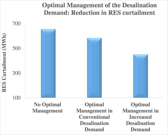
It shall be noted that resolving the DAS problem (i.e., minimise the objective function in (2), taking into account constraints (3)–(29)), while also considering the demand flexibility that can be offered by the desalination system (constraints (31)–(57)) will result in the grid absorbing the maximum amount of RES energy in order to serve the daily water demand. However, in order to further increase the RES produced energy injected in the grid, the RES energy within the day may be exploited in order to further increase the volume of water in the reservoirs of the desalination system. Thus additional clear water may be available in the end of the day that can potentially cover the water demand of the following days. This can be achieved by introducing the term $p_{sl,RES}{\displaystyle \sum }_{r=1}^{N_r}{\displaystyle \sum }_{t=1}^{N_t}\left(P_{max,r,t}-P_{r,t}\right)$ in the objective function (2), where $P_{max,r,t}$ indicates the maximum available RES energy and $P_{r,t}$ denotes the RES energy actually injected in the grid. A large penalty cost $p_{sl,RES}$ will result in a lower RES curtailment, $P_{max,r,t}-P_{r,t}$.

4. Study Case

In order to observe the potential benefits that can arise by managing the desalination system’s demand, the load for the year 2019 in the island of Kythnos is taken into account, as depicted in Figure 3. It is evident that significant variations are observed in the system load during the year. In particular, the tourism activity in the summer months significantly increases the system load, introducing a peak of 3.42 MW. A peak of 2.56 MW is also noted during April, denoting the Easter vacations in Greece when an increased tourism activity is observed.

In order to cover the island’s demand during the winter and summer days, while also ensuring the safe operation of the system, four conventional generators of a nominal power equal to 1.1 ΜW are installed in Kythnos Island. The four generators are identical, with the characteristics provided in

Table 1. Characteristics of the conventional production units in Kythnos.

Pmin	P1,max	P2,max
0.637 MW	0.8685 MW	1.1 MW
C0	C1	C2
144.8 €/h	191.3 €/h	239.1 €/h
Ramp-Up		Ramp-Down
0.6MW (per hour)		0.6MW (per hour)
Minimum Up Time		Minimum Down Time
1 h		1 h

. It is evident that two scales can be distinguished for the production of these generators (i.e., $k\in S=\left\{1,2\right\}$). The technical minimum power for the relevant units is equal to 637 kW, while the Ramp-up and Ramp-down requirements demand that the power between two hours cannot be increased (or decreased) more than 600 kW.

A wind generator of a nominal power equal to 600 kW is considered to be installed in Kythnos, with the production (P_max,t in (27)) as depicted in Figure 4. The limit R_l for the RES injected power in (28) is considered equal to 30%.

Concerning the desalination system in Kythnos, depicted in Figure 1, the maximum volume $\left\{V_{max,1},V_{max,2},V_{max,3},V_{max,4},V_{max,5},V_{max,6},V_{max,7}\right\}$ of the reservoirs is equal to $\left\{30,30,50,50,300,300 \mathrm{and} 30 {\mathrm{m}}^3\right\}$. It is evident that the Clear Water Reservoirs (Reservoirs No. 5 and 6) have quite an increased capacity for clear water ($V_{max,5}=V_{max,6}=300 {\mathrm{m}}^3$), indicating significant demand response capabilities. The nominal flow rate of the pumps and desalination units, as well as the relevant nominal power is indicated in

Table 2. Nominal flow rate and nominal power of the pumps and the desalination units in the desalination system.

Pump	Flow Rate (m3/h)	Power (kW)
sf1	72	11
sf2	72	11
fd1	120	22
fd2	120	22
pcw1	39	11
pcw2	39	11
bs1	72	11
bs2	72	11
Desalination Unit	Flow Rate (m3/h)	Power (kW)
ds1	12	35.5
ds2	12	35.5

.

The high and low limits in the reservoirs indicating the simple operation of the desalination system, not considering any smart demand response scheme to be applied, are presented in

Table 3. High and Low Levels for the reservoirs indicating the operation of the system when a smart DR scheme is not applied.

	Reservoirs 1 & 2	Reservoirs 3 & 4	Reservoirs 5 & 6	Reservoir 7
High Level (m3)	15	25	300	30
Low Level (m3)	13.5	22.5	270	27

Taking into account data provided for NIIs in Greece (https://www.deya-parou.gr/), the estimation of the yearly water demand in Merichas (the area in Kythnos where clear water from the desalination system is provided) is presented in Figure 5a. The distribution of the demand during the day is depicted in Figure 5b, according to data provided in [21].

5. Results

5.1. Simple Operation of the Desalination System

When the desalination system operates without applying any demand response scheme, the pumps and the desalination units only operate when the water in the reservoirs gets lower than the relevant low-level limit. The pumps and/or desalination units keep operating up until the water in the relevant reservoir reaches the required high-level limit.

For instance, considering the first day of the examined year, and taking into account that reservoirs 5 and 6 (the clear water reservoirs) in Figure 1 are filled up to an initial volume equal to 280 m³ each, the operation of the system can be observed in Figure 6. In this case the desalination system only operates when the water in reservoirs 5 and 6 gets lower than the relevant Low-Limit of 270 m³. The system operates up until the high-level limit of 300 m³ in these reservoirs is reached. The operation of the pumps and the desalination system providing water to the rest of the system’s reservoirs is also performed considering the relevant high and low-level limits of each respective reservoir. For instance, the volume of water in reservoirs 3 and 4 (the reservoirs where the clear water –or permeate- from the desalination system is initially stored) is depicted in Figure 6b. In this case, the desalination units are only required to operate three times during the day in order to respect the relevant High and Low-level limits in reservoirs 3 and 4.

Figure 6c depicts the volume of the sea water in reservoirs 1 and 2 in Figure 1. It is noted that a steady water volume among two consecutive hours does not necessarily mean that there is no water flowing in or out of the relevant reservoirs. For instance, for the 23rd hour of the examined day, reservoirs 1 and 2 are filled up until the maximum level. The system requires at this particular hour 38 m³ of sea water to flow out of these reservoirs, in order to be provided to the desalination units, reducing the relevant volume of sea water lower than the required low-limit. Thus, sea water is pumped towards reservoirs 1 and 2, as it can be observed in Figure 6c. The operational power of the relevant pumps is enough to fill the reservoirs up until the High-level within the examined hour.

The total energy requirements of the desalination system (energy demand for the operation of the desalination units and all the pumps in the system) is depicted in Figure 6d. Since the system operation is only considering the high and low-level rules described earlier, the operation of the system is not taking into account the available RES production. Thus, when applying the Day-Ahead Scheduling described in Section 2 for this specific day (i.e., the optimisation problem with the objective function (2) and constraints (3)–(29)), an amount of the available wind production will not be effectively exploited. In particular, significant amounts of wind energy are available, however, the desalination system cannot exploit this production as it can be observed in Figure 6d. For the specific day examined the total wind energy curtailed (i.e., the difference among the available wind production and the wind production finally injected in the grid) is equal to 5.14 MWh, or 47% of the total available wind production.

It shall be noted that the optimisation problem, concerning the results in this section, as well as the relevant optimisation problems in Section 5.2 and Section 5.3, have been solved using the modeling system GAMS, utilizing the CPLEX solver.

5.2. Smart Operation of the Desalination System Offering DR Services

In order to exploit the available wind production, while also taking into account the rest of the constraints linked with the operation of the conventional units in Kythnos, it is important to incorporate the operation of the desalination system within the optimisation problem of the Day-Ahead Scheduling. In this respect, constraints (31)–(57) are taken into account in the initial DAS problem described in Section 2. When applying the aforementioned optimisation problem for the day examined in Figure 6, it can be observed that the volume in the clear water reservoirs (reservoirs 5 & 6 in Figure 1) does not follow the water demand, as it is evident in Figure 7a. Similarly, the desalination units do not operate in order to satisfy the High and Low-level limits of the relevant reservoirs, as it is evident in Figure 7b. Instead the whole desalination system operates taking into account the optimal exploitation of the available wind production (in addition to the constraints linked with the operation of the desalination units).

The total energy required for the operation of the desalination system in this case is depicted in Figure 7d. It is evident that there are significant differences compared to the conventional operation of the desalination system in Figure 6d. In particular, the solution to the optimisation problem for the day examined, indicates the exact amount of energy required for the operation of the system at each specific hour in order for the produced wind energy to be effectively exploited.

Additionally the introduction of the term $p_{sl,RES}{\displaystyle \sum }_{r=1}^{N_r}{\displaystyle \sum }_{t=1}^{N_t}\left(P_{max,r,t}-P_{r,t}\right)$ in the objective function (2) results in further exploiting the RES production by increasing the volume of the clear water reservoirs at the end of the examined day (Figure 7a). It might not be necessary to fill these reservoirs, considering the relevant water demands, however, the additional RES production (Figure 7d) can be exploited to cover the relevant water demand of the next day(s).

It shall also be noted that a simple order from the system’s operator towards the desalination system to transfer a part of its energy among two hours could potentially not be performed, unless the capacity of the reservoirs has been optimally managed during the previous hours to allow the relevant increase/decrease in the demand. In particular, it is evident in Figure 7d that in order to effectively exploit the available wind production, an increase is required in the system’s demand during the last hour of the examined day. In order to achieve such an increase, the solution to the optimisation problem indicates that a lower water volume shall be available in reservoirs 1–6 during the previous hours (Figure 7a–c). However, when a non-scheduled operation is considered (Figure 6) the relevant reservoirs are already full during the hours preceding the last hour of the examined day, not allowing a significant increment in the system’s consumption. Thus, the DAS problem shall be fully aware of the capabilities of the desalination system in order to allow specific water flows (in and out of specific reservoirs) at specific hours of the day, allowing the optimal exploitation of the available RES produced energy.

For the examined day (Figure 6 and Figure 7), the effective exploitation of the desalination’s demand response capabilities results in reducing the RES curtailment to 4.89 MWh (a reduction equal to around 5% considering the initial RES curtailment of 5.14 MWh). Apparently, the capabilities for reducing the RES curtailment are linked with many parameters when resolving the Day-Ahead Scheduling, like the load of the system, constraints of the conventional generation units, available wind production, daily water requirements, etc.

In specific days the reduction of the RES curtailment that can be achieved may be much more significant than the one noted in the very first day of the examined year (Figure 6 and Figure 7). For instance, in August 29th significantly different energy and water needs are noted in the island of Kythnos. More specifically, the daily electricity needs as well as the relevant water demand are considerably increased due to the tourism activity in the island. In this specific day, it is evident in Figure 8a that the elasticity offered by the desalination system’s demand can significantly decrease the relevant RES curtailment. In particular, a reduction equal to around 42% is noted in this case in the curtailed wind production.

The importance of incorporating the operation of the desalination system within the Day Ahead Scheduling problem is also evident when closer inspecting Figure 8a and particularly the 9th hour of the day. Comparing the operation of the desalination system with and without the demand-response capabilities enabled, it appears that the optimisation problem in the former case suggests that a part of the desalination system’s demand shall be transferred from the 9th hour to the adjacent hours (8th and 10th hour), in order to better exploit the available wind production during these hours.

However, the decrease in the desalination’s system demand during the 9th hour also allows more wind energy to be injected in the grid. More specifically, when considering the non-scheduled operation of the desalination system, the initially increased demand of the whole island at the 9th hour of the examined day requires that the system’s energy is supplied by two conventional generators as it is evident in Figure 8b. More specifically, the Day-Ahead Scheduling (according to constraints linked with the operation of conventional units, safety limits for the power injected from RES production units, etc.) indicates that a second generator is required to start operating in order to cover the island’s demand. In this case, the RES produced energy cannot be fully exploited resulting in an increased RES curtailment at this specific hour, as it is evident in Figure 8b.

However, when the operation of the desalination system is considered alongside the relevant DAS problem (according to the methodology proposed in Section 3), the reduction of the desalination system’s demand during the 9th hour is enough to avoid the operation of the second conventional unit at this specific hour (Figure 8c). More specifically, the power production from the 1st unit in addition to the available RES produced energy, is enough in this case to sufficiently cover the island’s demand, resulting in a zero RES curtailment during this hour.

It is, therefore, evident that the exploitation of the desalination’s demand is not a simple problem that can be resolved by a mere reduction or increase in the systems demand. In particular, it is important to incorporate the management of the desalination system within the DAS problem in order to be fully aware of the system’s management capabilities. In this respect, the effective operation of the desalination system while also taking into account parameters linked with the DAS, will allow specific variations in the system’s demand that can avoid the operation of additional conventional units, while better exploiting the available RES production.

The application of the DAS for all the days of the examined year, indicates that a significant reduction can be achieved in the curtailed wind production. In particular the initial wind curtailment of 655 MWh can be reduced to 583 MWh, indicating a reduction equal to around 11%. The relevant increase in the RES production injected in the grid is equal to around 5%.

5.3. Employment of the Desalination System to Cover the Whole of Kythnos’ Water Demand

Better results for the RES energy injected in the grid can be achieved in case the demand of the desalination system is increased. In particular, the examined desalination system that is currently providing water to the population of Merichas, could be employed to provide water to the whole island of Kythnos. It can be observed that the conventional operation of the system (according to the high and low-level limits in the reservoirs) can satisfy more than 87% of the island’s yearly water needs.

In this case the operation of the desalination system introduces a significant energy demand. However, when considering the conventional operation of the system, according to the high and low levels of the relevant reservoirs, this demand cannot always be covered with the available RES production. For instance, for the day depicted in Figure 9a, the conventional operation of the desalination system (red line in the figure) indicates an increased energy demand for many hours of the day, yet this demand does not always coincide with the RES curtailment. However, the incorporation of the system’s operation within the DAS problem allows a better management of the desalination system’s operation, with a demand optimally distributed in the day in order to effectively exploit the available RES production. In this case the curtailed RES production can be decreased by more than 22%.

For days with an extremely high water demand (Figure 9b), the conventional non-scheduled operation of the desalination system indicates that the desalination system shall constantly operate with a steady demand during the day, to retain the required high and low level limits in all the reservoirs. However, when considering a scheduled operation of the desalination system, according to the methodology proposed in this paper, the capacity of the reservoirs can be effectively exploited in order to introduce slight variations in the energy demand that can better exploit the available RES production. Such variations can effectively reduce the RES curtailed energy by around 29% in the day examined in Figure 9b.

When the proposed optimisation problem in Section 3 is applied for the whole year of 2019, the RES curtailment can be reduced from 0.58MWh to 0.45 MWh, indicating a reduction greater than 22%. The energy required from conventional units in this case is reduced from 8.91 GWh to 8.77 GWh.

When considering the conventional operation of the desalination system, the network can absorb the whole daily amount of the produced RES energy (i.e., the maximum available RES production during the day) for a total amount of 30 days. However, when considering the application of the proposed optimisation procedure the relevant number of days is increased to 51.

6. Discussion

An optimisation procedure is proposed in this paper for the optimal management of the demand of a desalination system in a non-interconnected island, taking into account parameters linked with the day-ahead scheduling. The application of this optimisation procedure on the examined study–cases indicates quite significant results in achieving a greater RES penetration in the examined island. Future work on the proposed optimisation procedure could potentially include a brine discharge rate in order to minimize the relevant environmental impacts.

In order to allow the integration of the proposed optimisation process in the operation of a desalination system, appropriate modifications shall be realized on the operation of the system’s pumps and desalination units. More specifically, the desalination units as well as the relevant pumps shall no longer operate according to the High/Low level limits in the reservoirs, but shall be modified to operate according to the optimal management procedure described in this paper.

The examined study case for the application of the optimisation method proposed in this paper concerns the desalination units installed on the island of Kythnos and the installation of a 600 kW wind generator with the production profile depicted in Figure 4. Other study cases, like the installation of other RES units, could potentially lead to different results due to the different production profiles, compared to the one of the wind generator in Figure 4. In any case, however, the proposed optimisation procedure could be applied for any study-case of RES units in order to indicate the optimal operation of the desalination system.

7. Conclusions

This paper proposes a novel methodology to define the optimal management of a desalination system’s demand within the framework of the Day-Ahead Scheduling rules considered in NII systems. The proposed methodology has been applied for the desalination system in the Greek Non-Interconnected Island of Kythnos that supplies clear water to the community of Merichas. The results of the analysis indicate that the conventional operation of the desalination system can potentially lead to significant amounts of curtailed RES energy. However, the efficient management of the desalination system’s operation, allowing specific water flows, in and out of specific reservoirs, at specific hours of the day, can increases the RES penetration in the examined system. In particular, the RES curtailment can be decreased from 655 MWh to 583 MWh, when considering the operation without and with the proposed optimisation procedure respectively. The relevant increase in the RES produced energy injected in the grid is equal to around 5%.

The increment in the RES injected energy is much more significant in case the desalination system is required to supply water to the whole island of Kythnos. More specifically, the application of the proposed optimisation procedure for the whole year of 2019, indicates that the RES curtailment can be reduced from 0.58 GWh to 0.45 GWh (i.e., a reduction greater than 22%).

Moreover, according to the results of the analysis presented in this paper, it is quite significant to consider the optimisation of the desalination demand management alongside the constraints of the day-ahead scheduling. More specifically, the right amount of decrement in the desalination system’s demand can lead to a better exploitation of the available RES production, by avoiding the operation of additional conventional units. Thus, the Day-Ahead Scheduling problem shall be fully aware of the capabilities of the desalination system in order to allow the optimal exploitation of the available RES produced energy.

References

1. Li, Z.; Siddiqi, A.; Anadon, L.D.; Narayanamurti, V. Towards sustainability in water-energy nexus: Ocean energy for seawater desalination. Renew. Sustain. Energy Rev. 2018, 82, 3833–3847. [Google Scholar] [CrossRef] [Green Version]
2. Li, W.; Krantz, W.B.; Cornelissen, E.R.; Post, J.W.; Verliefde, A.R.; Tang, C.Y. A novel hybrid process of reverse electrodialysis and reverse osmosis for low energy seawater desalination and brine management. Appl. Energy 2013, 104, 592–602. [Google Scholar] [CrossRef]
3. Oikonomou, K.; Parvania, M. Optimal Participation of Water Desalination Plants in Electricity Demand Response and Regulation Markets. IEEE Syst. J. 2019. [Google Scholar] [CrossRef]
4. Okampo, E.J.; Nwulu, N.I. Optimal energy mix for a reverse osmosis desalination unit considering demand response. J. Eng. Des. Technol. 2020. [Google Scholar] [CrossRef]
5. Malisovas, A.; Koutroulis, E. Design Optimization of RES-Based Desalination Systems Cooperating with Smart Grids. IEEE Syst. J. 2019. [Google Scholar] [CrossRef]
6. Wu, B.; Maleki, A.; Pourfayaz, F.; Rosen, M.A. Optimal design of stand-alone reverse osmosis desalination driven by a photovoltaic and diesel generator hybrid system. Sol. Energy 2018, 163, 91–103. [Google Scholar] [CrossRef]
7. Amin, Z.M.; Maswood, A.I.; Hawlader, M.N.A.; Al-Ammar, E.A.; Orfi, J.; Al-Ansary, H.A. Desalination With a Solar-Assisted Heat Pump: An Economic Optimization. IEEE Syst. J. 2013, 7, 732–741. [Google Scholar] [CrossRef]
8. Song, Y.; Liu, Y.; Wang, R.; Ming, M. Multi-Objective Configuration Optimization for Isolated Microgrid With Shiftable Loads and Mobile Energy Storage. IEEE Access 2019, 7, 95248–95263. [Google Scholar] [CrossRef]
9. Qi, W.; Liu, J.; Christofides, P.D. Supervisory Predictive Control for Long-Term Scheduling of an Integrated Wind/Solar Energy Generation and Water Desalination System. IEEE Trans. Control Syst. Technol. 2012, 20, 504–512. [Google Scholar] [CrossRef]
10. Bilton, A.; Kelley, L.C.; Dubowsky, S. Photovoltaic reverse osmosis—Feasibility and a pathway to develop technology. Desalin. Water Treat. 2011, 31, 24–34. [Google Scholar] [CrossRef]
11. Ali, I.B.; Turki, M.; Belhadj, J.; Roboam, X. Optimized fuzzy rule-based energy management for a battery-less PV/wind-BWRO desalination system. Energy 2018, 159, 216–228. [Google Scholar]
12. Rezk, H.; Al-Dhaifallah, M.; Hassan, Y.B.; Ziedan, H.A. Optimization and Energy Management of Hybrid Photovoltaic-Diesel-Battery System to Pump and Desalinate Water at Isolated Regions. IEEE Access 2020, 8, 102512–102529. [Google Scholar] [CrossRef]
13. Guo, L.; Liu, W.; Li, X.; Liu, Y.; Jiao, B.; Wang, W.; Wang, C.; Li, F. Energy Management System for Stand-Alone Wind-Powered-Desalination Microgrid. IEEE Trans. Smart Grid 2016, 7, 1079–1087. [Google Scholar] [CrossRef]
14. Frangioni, A.; Gentile, C.; Lacalandra, F. Tighter Approximated MILP Formulations for Unit Commitment Problems. IEEE Trans. Power Syst. 2009, 24, 105–113. [Google Scholar] [CrossRef] [Green Version]
15. Wu, L. A tighter piecewise linear approximation of quadratic cost curves for unit commitment problems. IEEE Trans. Power Syst. 2011, 26, 2581–2583. [Google Scholar] [CrossRef]
16. Mohammadi, F.; Sahraei-Ardakani, M.; Al-Abdullah, Y.M.; Heydt, G.T. Coordinated Scheduling of Power Generation and Water Desalination Units. IEEE Trans. Power Syst. 2019, 34, 3657–3666. [Google Scholar] [CrossRef]
17. Tigrine, Z.; Aburideh, H.; Abbas, M.; Hout, S.; Merzouk, N.K.; Zioui, D.; Khateb, M. Membrane Desalination Technology in Algeria: Reverse Osmosis for Coastal Areas. In Exergy for a Better Environment and Improved Sustainability 2; Springer: Berlin/Heidelberg, Germany, 2018. [Google Scholar]
18. Liu, T.; Sheu, H.Y.; Tseng, C.N. Environmental impact assessment of seawater desalination plant under the framework of integrated coastal management. Desalination 2013, 326, 10–18. [Google Scholar] [CrossRef]
19. Musthafa, M.O.; Chabib, C.M.; Mustafa, I.; Al Ghaferi, A.; AlMarzooqi, F. Brine management in desalination industry: From waste to resources generation. Desalination 2019, 472, 114187. [Google Scholar]
20. Alameddine, I.; El-Fadel, M. Brine discharge from desalination plants: A modeling approach to an optimized outfall design. Desalination 2007, 214, 241–260. [Google Scholar] [CrossRef]
21. Cole, G.; Stewart, R.A. Smart meter enabled disaggregation of urban peak water demand: Precursor to effective urban water planning. Urban Water J. 2003, 10, 174–194. [Google Scholar] [CrossRef] [Green Version]
Figure 1. Overview of the desalination system installed in Kythnos.
Energies 13 04021 g001
Figure 2. Current operation of the desalination system in Kythnos, according to the High and Low-Level of each Reservoir.
Energies 13 04021 g002
Figure 3. Load of Kythnos Island in 2019.
Energies 13 04021 g003
Figure 4. Wind Production during the examined year.
Energies 13 04021 g004
Figure 5. (a) Water demand in Merichas for each period of the year and (b) distribution of the water demand during the day [21].
Energies 13 04021 g005
Figure 6. Conventional operation of the desalination system for the first day of the examined year: (a) Volume of water in the clear water reservoirs and the relevant water demand, (b) energy demand of the desalination units and volume of permeate water, (c) energy demand for pumping sea water and the relevant volume of sea water in reservoirs 1 & 2, (d) Curtailment of the wind production & desalinations system demand.
Energies 13 04021 g006
Figure 7. “Smart” operation of the desalination system for the first day of the examined year: (a) Volume of water in the clear water reservoirs and the relevant water demand, (b) energy demand of the desalination units and volume of permeate water, (c) energy demand for pumping sea water and the relevant volume of sea water in reservoirs 1 & 2, (d) Curtailment of the wind production & desalinations system demand.
Energies 13 04021 g007
Figure 8. Operation of the desalination system with and without the relevant DR capabilities in 29/08/2019: (a) Comparison of the RES curtailment and the desalination system demand, (b) operation of the conventional generators without the DR capabilities of the desalination system enabled, and (c) operation of the conventional generators when the desalinations system offers demand response services.
Energies 13 04021 g008
Figure 9. Comparison of the RES curtailment and the desalination system demand, when the desalination system satisfies the water requirements of the whole island of Kythnos. Operation with & without the relevant DR capabilities for (a) 06/01/2019 and (b) 13/07/2019.
Energies 13 04021 g009