Optimization Wells Placement Policy for Enhanced CO₂ Storage Capacity in Mature Oil Reservoirs

Abstract

One of the possibilities to reduce carbon dioxide emissions is the use of the CCS method, which consists of CO₂ separation, transport and injection of carbon dioxide into geological structures such as depleted oil fields for its long-term storage. The combination of the advanced oil production method involving the injection of carbon dioxide into the reservoir (CO₂-EOR) with its geological sequestration (CCS) is the CCS-EOR process. To achieve the best ecological effect, it is important to maximize the storage capacity for CO₂ injected in the CCS phase. To achieve this state, it is necessary to maximize recovery factor of the reservoir during the CO₂-EOR phase. For this purpose, it is important to choose the best location of CO₂ injection wells. In this work, a new algorithm to optimize the location of carbon dioxide injection wells is developed. It is based on two key reservoir properties, i.e., porosity and permeability. The developed optimization procedure was tested on an exemplary oil field simulation model. The obtained results were compared with the option of arbitrary selection of injection well locations, which confirmed both the legitimacy of using well location optimization and the effectiveness of the developed optimization method.

1. Introduction

Some scientists confirm the relationship between the emission of greenhouse gases into the atmosphere and the increase of average temperature on Earth. Opponents of this theory rely on analyses proving that such fluctuations have occurred on the planet over thousands of years [1]. However, both the narrator for this theory and opponents agree that possible countermeasures should be implemented to reduce emissions. One of the potential options for reducing carbon dioxide emissions is the use of the CCS method, which consists of CO₂ separation, transport, compression and CO₂ injection for its long-term storage in geological structures as well as monitoring CO₂ behavior in the structure. In general, this process can be divided into several stages. The first one involves the capture of carbon dioxide from exhaust gases produced by emitters. The best source is the most common source—fossil fuel power plants, e.g., coal—due to the amount of carbon dioxide emitted, availability and efficiency of the process. Carbon dioxide separation is carried out using three main processes called: post-combustion, pre-combustion and oxy-fuel combustion [2]. The post-combustion method involves the separation of carbon dioxide from producing exhaust gases. On the other side, pre-combustion is a process in which CO₂ capture occurs before the mixture is burned. An alternative method to the above mentioned is the use of fossil fuel combustion in pure oxygen—oxy-fuel combustion [3]. Due to the distance between the emitter and the field, separated carbon dioxide can be delivered using road, rail, water or pipeline, which guarantees the lowest cost [2]. The final stage is the injection of pressurized carbon dioxide into the field to store it in the reservoir rock. Carbon dioxide can be stored not only in partially depleted oil and gas reservoirs but also in aquifers and unexploited coal beds. In each case, it is important to use certain physical properties of carbon dioxide that vary with pressure and temperature. Carbon dioxide in the supercritical phase is characterized by the density of the liquid and the viscosity and compressibility of the gas, which is crucial in terms of its underground storage. Another important issue in the storage of carbon dioxide in geological structures is the isolation of CO₂ preventing its penetration into undesirable rock formations [4]. In the case of depleted petroleum reservoirs, the capacity of the reservoir is limited by the pressure. The injection of carbon dioxide continues until the reservoir pressure is reached. Moreover, pressure cannot also exceed the fracturing pressure of the source rock. These values cannot be exceeded due to the fact that there is a possibility of the destruction of impermeable layers of the structure and as a result of penetration of carbon dioxide to undesirable rock formation [4].

One of the possible CCS process realizations is the use of depleted oil fields for the storage of carbon dioxide. Three main production methods that are used to recover oil from the reservoir include primary, secondary and tertiary methods. These methods sequentially allow for a gradual increase in the reservoir recovery factor, which is associated with increasing costs and the complexity of the process. In the case of primary methods, oil is produced from the reservoir using natural reservoir energy in the form of pressure in the reservoir, which allows obtaining a recovery factor of 20–30% [5]. The implementation of secondary methods supplying additional energy to the reservoir structure by water or gas injection into the reservoir [6] allows an increase of recovery factor by about 10% compared to the primary methods. To further increase the recovery factor, tertiary methods, also known as Enhanced Oil Recovery (EOR) methods, are used [7]. They consist in affecting the oil properties, including viscosity and density, as well as the supply of energy supporting the production process. One of the increasingly considered tertiary methods is the CO₂-EOR method involving the injection of carbon dioxide into partially depleted oil fields. This method can be applied in three different ways because CO₂ injection can be continuous, cyclic or water alternating [8]. In continuous CO₂ flooding, carbon dioxide is injected at the injector and oil is produced at the producer continuously. In this process, the miscibility development between CO₂ and oil is obtained thanks to the multicontact process, through condensing or vaporizing mechanisms, or, as in most scenarios, a combination of them [8]. In contrast to the continuous CO₂ injection, in the cyclic process (huff-n-puff), only one well is involved, which serves both the injection of CO₂ and the production of oil. This process is composed of three stages: huff (CO₂ injection period), soak (well shut-in period during which CO₂ swells oil and lowers oil viscosity) and puff (oil production period) [8]. Water Alternating Gas (WAG) is a process in which CO₂ injection and water injection are carried out alternately over a period of time. In the WAG process, the mobility ratio between CO₂ and oil is reduced, which is favorable because it delays gas breakthrough [8]. In general, the main advantage of the CO₂-EOR process is the change in crude oil properties by reducing viscosity and surface tension [9]. In addition, it is possible to combine this process with carbon dioxide geological sequestration (CCS) implemented after the end of the EOR process to obtain additional environmental benefits. This combination is called the CCS-EOR process, which can be separated into two stages [2]: CO₂ Enhanced Oil Recovery (CO₂-EOR) and Carbon Capture and Storage (CCS).

To achieve the best ecological and economic effects, it is important to maximize the storage capacity for CO₂ injected in the CCS phase. To achieve this state, it is necessary to maximize the recovery factor during the CO₂-EOR phase. One of the key factors affecting the efficiency of crude oil production when implementing the CCS-EOR method is the appropriate selection of CO₂ injection wells locations. This choice is very complicated because the number of potential solutions increases non-linearly with the increase of parameters on which this choice depends. These include, among others: the geological structure of the rock or the properties of fluids in the reservoir. These factors affect fluid flow in the reservoir in a non-linear way, which causes that the issue of location optimization requires consideration of many parameters and analysis of many cases to determine the best coordinates for injection wells [10].

2. Well Location Optimization

Optimization of wells location by defining the number, type and location of perforation is a critical element of the hydrocarbon reservoir management plan [11]. The problem of optimal location is strongly non-linear, and its complexity increases when in addition to traditional vertical wells horizontal, directional or multilateral wells are considered [12]. Nowadays, well placement is carried out on three-dimensional geological models, which can contain hundreds of layers and millions of cells with variable properties, which means that the selection of optimal zones is not trivial and may be impossible without the use of multidimensional optimization methods. Optimization methods used in reservoir engineering by their mode of operation can be divided into [13]: (I) gradient; and (II) gradientless. Information on the objective function gradient is obtained using the adjoint gradient method or the finite difference method.

In the case of gradient methods, the steepest descent algorithm where the gradient information is obtained using the adjoint gradient method is most often used and widely described in the works [14,15,16,17,18]. Zandvliet et al. [19] used the steepest descent method in combination with the adjoint gradient method to optimize the wells location. The location of injection wells on a two-dimensional grid of an artificial reservoir was optimized, in which the production wells had a fixed location. The authors conducted numerical experiments, which confirmed that the quality of the solution depends on the starting point of the algorithm, which translates into a conclusion about the multimodality of the objective function in the case of optimization of the wells location.

Wang [20], using the two-dimensional model of the reservoir, considered the location of injection wells to maximize the value of the objective function linking the cash flows associated with production and injection with the incurred costs of drilling a new injection well. The assumption of the optimization task involves determining such a vector of decision variables consisting of individual injection costs, which maximizes the adopted objective function. In the first stage of the algorithm, an injection well is located in each cell that does not contain a production well. The performance of individual wells is modified using the steepest descent method, in which the direction of change is calculated directly based on the objective function gradient. If the performance of an individual well drops to zero, the well is removed from the simulation. The injection rates of individual wells as well as their production rates remain unchanged during production. The result is an optimal number of injection wells and their location. A limitation of the method proposed by Wang [20] is the simplification of the reservoir structure into a two-dimensional form. In each iteration of the algorithm, only one well is removed, which can translate into low time efficiency of calculations and can be inefficient in the case of large-scale problems.

Forouzanfar [21] proposed a two-step solution to the problem of optimization of the number and location of wells using the gradient method. Optimization calculations were carried out on a three-dimensional model of the reservoir, considering the possibility of three-phase flows. The optimization objective function is a modified and extended form of the function proposed by Wang [20]. The presented solution improves the time efficiency of calculations by simultaneous optimization of the number and position of both production and injection wells.

The idea of using virtual wells (additional, non-existent wells located around the considered well, located in adjacent cells of the simulation model) to optimize the position of the actual vertical well has found application in determining the optimal horizontal well trajectory. Vlemmix et al. [22] proposed the use of short and perforated pseudo “side-tracks” to determine the direction in which the current, real trajectory should be moved.

The use of a numerical simulator to describe the fluid flow in the pore space of a hydrocarbon reservoir significantly hinders the analysis of the objective function in terms of the occurrence of extremes. In the case of well allocation problems, decision variables are represented by integers corresponding to block numbers in the simulation model, hence decision variables are not continuous. In addition, it should be noted that gradient optimization methods only work in solving problems in which the objective function is unimodal. The characteristics of the operation of these methods do not allow abandoning the local extreme and temporarily deteriorating of the objective function value. The solution to this problem may be the use of multi-start technique, which runs the optimization algorithm from different starting points. However, when the objective function has many near-extreme extremes, the probability of hitting the global extreme attraction area is low. The solution to these types of problems are algorithms that do not use a gradient in their operation, which can generally be divided into two main groups [23]: (I) local search algorithms; and (II) global search methods, e.g., population algorithms.

Optimization based on a genetic algorithm often finds use in the process of the new vertical production wells [10,24,25,26,27] or wells with complicated topology [28,29,30] location optimization. The use of the particle swarm algorithm for typing the location of vertical and unconventional wells was presented by Onwunalu and Durlofsky [31]. The group of stochastic algorithms includes the simulated annealing algorithm used in [32]. The algorithm is responsible for the optimal placement of wells and determining their operation schedule. In the case of large-scale problems, optimization of the individual well’s location is computationally demanding and time-inefficient [33]. Reducing the size of the optimization problem involves introducing certain well patterns [34,35,36,37].

3. Developed Wells Location Optimization Procedure

In this work, a new algorithm to optimize the location of wells injecting carbon dioxide into the oil field is developed. A deep analysis of the literature shows that there is no clear information which reservoir rock properties have a greater impact on fluid flow in the reservoir [38]. With the increase in the simulation model’s detail, the complexity of the problem of wells optimal allocation increases, and the developed numerical methods become ineffective due to the need to search a large space of potential solutions. An attempt to solve this problem is to associate the location with the petrophysical properties of the reservoir. Based on the analysis of the literature, the method developed in this work considers two key parameters characterizing reservoir properties: porosity and permeability. Their values are assigned to each block of the numerical simulation model of the reservoir. To automate the process of optimizing the selection of injection well coordinates, the developed algorithm was implemented in Matlab, which was combined with the Schlumberger Eclipse Simulation numerical reservoir simulator. In addition, in this study, it was checked which of these parameters has a greater impact on the selection of the optimal location of CO₂ injection wells.

Carbon dioxide injection should be carried out in areas with the best reservoir properties [38]. These areas allow gas to easily penetrate to further regions of the reservoir, which facilitates the process of mixing carbon dioxide with oil and as a result improves the efficiency of the CO₂-EOR process. Due to the presence of an oil–water contour in the reservoir, in the proposed algorithm, the search area for the location of the injection wells is limited to the region where only the oil phase occurs. This area is then evenly divided into $r$ number of parts, so-called “mini regions”, containing the same number of simulation model cells. Thanks to this division, the algorithm checks more points in a given iteration because the simulation is run not only for the best location selected from the entire reservoir but also for the best location in each “mini region”. Therefore, $r$ times more locations are tested, which increases the probability of finding the optimal location of the injection well. An example of dividing the reservoir into 9 ($r$ = 9) “mini regions” is presented in Figure 1.

In addition, it was assumed that the proposed algorithm will check the possibility of locating injection wells in places with coordinates where the weighted average considering porosity and permeability in this location is the largest. A block diagram of the created algorithm is presented in Figure 2.

In subsequent iterations of the algorithm, weights are first assigned for porosity and permeability. In the first step, the weights are 0 and 1, which means that in this case only permeability is taken into account. In the next steps, the weight for porosity is increased by 0.1 and for permeability is reduced by the same value, according to the following relationships:

• porosity:

  $$\{\begin{array}{c}w{\varphi }_1=0 \\ w{\varphi }_i=w{\varphi }_{i-1}+0.1\wedge i>1\end{array}$$

  (1)

  where $w\varphi$ is the porosity weight and $i$ is the iteration number.
• permeability:

  $$\{\begin{array}{l}w{k}_1=1\\ w{k}_i=w{k}_{i-1}-0.1\wedge i>1\end{array}$$

  (2)

  where $wk$ is the permeability weight and $i$ is the iteration number.

Due to differences in the order of magnitude between porosity, e.g., 0.13, and permeability, e.g., 200 mD, these values are initially normalized within the designated “mini regions” using the following relationship:

$$a_n=\frac{a-a_{min}}{a_{max}-a_{min}}$$

(3)

where $a_n$ is the normalized value of the feature, $a$ is the value of this feature, $a_{min}$ is its minimum value and $a_{max}$ is its maximum value.

As a result of data normalization, the permeability and porosity values in the range $\langle 0, 1\rangle$ are obtained, which allows them to be compared.

Then, a weighted average is calculated for a given weight ratio in each possible location (x, y) of the potential well for each of the mini regions based on the following formula:

$${\mu }_i=w{\varphi }_i·{\overline{\varphi }}_n+w{k}_i·{\overline{k}}_n$$

(4)

where $\mu$ is the weighted average, $i$ is the iteration number, $w\varphi$ is the porosity weight, ${\overline{\varphi }}_n$ is the normalized porosity average value, $wk$ is the permeability weight and ${\overline{k}}_n$ is the normalized permeability average value.

Average values of normalized porosity and permeability appearing in Equation (4) are calculated for a given set of coordinates (x, y) as arithmetic means over the entire thickness of the reservoir based on the values of these parameters exported for each block of the reservoir simulation model. Data normalization enables the elimination of the impact of only one of the reservoir rock properties on the weighted average value due to its larger order of magnitude.

After calculating the weighted average values for all analyzed coordinates, the coordinates with the highest average value in each mini region are automatically saved to the T vector. Therefore, this vector in each iteration is supplemented with the coordinates (x, y) of $r$ points according to the following relationship:

$${\forall }_{j\in 1..r}\mathit{max}{\left({\mu }_i\right)}_j\to T_{i,j}=P_{i,j}\left(x_{i,j};y_{i,j}\right)$$

(5)

where $j$ is the region number, $r$ is the number of “mini regions”, $\mu$ is the weighted average, $i$ is the iteration number, $T$ is $P$ points vector, $P$ is the best point in a given mini region, $x$ is the x coordinate of the block and $y$ is the y coordinate of the block.

To increase the computational efficiency of the algorithm, after saving the results to the vector, it is checked whether the set of coordinates found in a given iteration is no longer present with a different weight ratio of porosity and permeability in accordance with the following relationship:

$$if T_i\in A_i\mathrm{then}{A}_{i+1}=A_i\mathrm{else}{A}_{i+1}=A_i{{\displaystyle \cup }}^{}\left\{T_i\right\}$$

(6)

where $T$ is $P$ points vector ($P$ is the best point in a given mini region), $i$ is the iteration number and $A$ is a set of unique vectors $T$.

If a given combination did not occur before, then the whole $T$ vector is added to the initially empty set of unique solution sets ($A$). However, if the result is a repetition of an already calculated one, then the given coordinate set is stored, but it is not taken into account in further stages of the algorithm.

The above operation completes a single iteration followed by a change in weights for porosity and permeability. The whole scheme is repeated eleven times, i.e., until the average value is calculated only based on porosity, because its weight will be 1 and the weight for permeability will be 0.

The next step of the proposed calculation procedure is to automatically run the reservoir simulator for each point from each $T$ vector saved to set $A$. Therefore, the number of simulations performed can be reduced by omitting repeated sets of solutions in further considerations, which significantly speeds up the algorithm’s execution time. To run a simulation for a given injection well location, its coordinates are saved to the functions defining new wells in the simulator, after which the simulation is automatically started for the updated input file. After the simulation, the value of cumulative oil production obtained at a given location of the injection well is automatically saved. This process is repeated until the simulation is run for all mini regions (for all porosity and permeability weight ratios).

All cumulative oil production values obtained as a result of the carried out reservoir simulations are then compared. For the analyzed area of the reservoir, such coordinates are finally selected for which the location of the injection well guarantees obtaining the largest production of crude oil during the CO₂-EOR process, maximizing the recovery factory, which is equivalent to maximizing CO₂ storage capacity.

4. Case Study

The created optimization procedure was tested on a simulation model of the oil reservoir exploited since the end of the 19th century. The main mineral is crude oil with the specific gravity from 840 to 843 kg/m³, while the natural gas is present in the reservoir in trace amounts. The considered reservoir is divided into two oil and natural gas horizons. The first horizon consists of three regions, separated from each other by faults, drilled successively with 15, 6 and 5 production wells. In Region 3, there is also one injection well injecting the reservoir water. The second horizon of the reservoir includes Region 4 drilled through one production well, hence it is not considered for carbon dioxide injection. The division of the analyzed oil reservoir into regions is presented in Figure 3.

To apply the developed optimization procedure, the porosity and permeability distributions presented in Figure 4 and Figure 5 were analyzed. The porosity distribution is very diverse—the highest values, within 13%, are in the central part of each region, while the lowest values, at 2%, characterize areas at the reservoir boundaries and in its deeper layers. The permeability of the reservoir is characterized by an even distribution. Most of the reservoir has a permeability of few mD, which makes difficulties during fluid flow. The only place where the values are higher is the southeastern part of the reservoir, but oil saturation is very low there.

The detailed characteristics of the analyzed reservoir are presented in our previous work [39], confirming the potential of the CCS-EOR method implementation on this reservoir. In this work [39], a maximum CO₂ storage capacity of 50 million m³ was determined and the efficiency with which carbon dioxide could be supplied from the emitter throughout the entire period of the CO₂-EOR and CCS process was established at 5000 m³/day. To implement the CCS-EOR method on the analyzed reservoir, it was proposed to use the existing water injection well and to drill one new injection well in each of the three regions (Regions 1–3), through which carbon dioxide will be injected into the reservoir rock structure. This paper [39] proposes a CCS-EOR process scheme taking into account the arbitrary selection of new injection wells locations based on literature knowledge [40] as well as the distribution of reservoir rock and reservoir fluid properties and preliminary simulation analyses performed. In addition, re-injection of the produced mixture of gases (containing both natural gas and CO₂) and closing of production wells when the molar fraction of carbon dioxide in the extracted fluid exceeds 0.9 was assumed. The economic limit for oil production was set at 3 m³/day. Its achievement completes the CO₂-EOR stage and begins the process of carbon dioxide storage, in which CO₂ injection is carried out until reaching pressure limits in each region of 77, 67 and 80 bar, respectively.

The cited work [39] is the basis of these considerations and represents the base option for conducting the CCS-EOR process on the analyzed reservoir—the arbitrary scenario. However, in this paper, to increase the CO₂ storage capacity, the base option is extended to optimize the location of injection wells using the optimization procedure proposed by the authors—the optimal scenario. For comparative purposes, other assumptions remain unchanged relative to the variant with an arbitrary selection of well locations. The scheme of division into mini regions and the developed optimization algorithm was applied to all three regions that required drilling of an injection well to implement the CCS-EOR method. In addition, an analysis of the effect of porosity and permeability on the results obtained in the optimization process was also made. For this purpose, charts of cumulated production depending on the permeability and porosity weights for all three regions were drawn. In addition, tables in which weights for location coordinates that have been duplicated are also prepared. Repeated results for each of the analyzed regions are marked in the corresponding tables with the same color.

5. Optimization Results

For Region 1, reservoir simulations were calculated only for five coordinate sets from mini regions (Figure 6). Thus, the omission of repetitive solutions has significantly improved and shortened the operation of the algorithm. In this region, the maximum production at 63,690 m³ determining the optimal location of the injection well was obtained for a permeability weight of 0.8 and a weight of porosity of 0.2. In addition, it can also be seen in Figure 6 that most of the simulations were performed for higher permeability weights than porosity weights.

Table 1. Considered weights including repetitions for Region 1. Repeated results are marked with the same color.

No.	Permeability	Porosity
1	1	0
2	0.9	0.1
3	0.8	0.2
4	0.7	0.3
5	0.6	0.4
6	0.5	0.5
7	0.4	0.6
8	0.3	0.7
9	0.2	0.8
10	0.1	0.9
11	0	1

shows that in the first four weights sets the coordinates were not repeated. For the remaining steps, the coordinates do not change despite the increase in the porosity weight and the results obtained are the same as for the weight ratio 0.6:0.4 (Figure 6). This means that in the case of Region 1 the permeability of reservoir rock has a greater impact on the results obtained.

Results obtained for Region 2 (Figure 7) are characterized by a different relationship than those obtained for Region 1. In this case, simulations were run for up to seven different weights, which indicates a large diversity of analyzed properties in this region of the reservoir. The maximum cumulated oil production at 31,733 m³ was obtained for the permeability to porosity weights ratio of 0.4:0.6.

Table 2. Considered weights including repetitions for Region 2. Repeated results are marked with the same color.

No.	Permeability	Porosity
1	1	0
2	0.9	0.1
3	0.8	0.2
4	0.7	0.3
5	0.6	0.4
6	0.5	0.5
7	0.4	0.6
8	0.3	0.7
9	0.2	0.8
10	0.1	0.9
11	0	1

shows that the same value also characterizes the set of weights 0.3:0.7, but, in both cases, porosity has a greater impact on the optimal location of the injection well. Moreover, Region 2 is relatively small compared to others. The area of the region is about half the size of Region 1 and a quarter the size of Region 3. This causes the distance between the injection well and the production well to also be small. It can therefore be concluded that this reduces the impact of permeability on oil production.

Table 2 shows that the results are repeated less regularly than in Region 1. However, the same coordinates are obtained for successive weights. For Region 2, there are three sets of duplicate results. The same coordinates were determined for a weight ratio of 0.7: 0.3 and 0.6:0.4. The second repeating pair are weights 0.4:0.6 and 0.3:0.7. The same results also characterize the last three possibilities. It confirms the large variety of considered reservoir properties in the analyzed region.

Analyzing the results obtained for Region 3 (Figure 8), an analogous relationship can be observed as for Region 1. Simulations were made only for four sets of weights, which confirms the validity of the included omission of duplicate coordinates. The maximum production determining the optimal location of the injection well was 31,619 m³ with the permeability to porosity weight ratio of 0.7:0.3.

Similar to the situation in Region 1, non-repetitive results were obtained for high permeability weights, which proves its greater impact on the location of the injection well. The same results as for Set 4 with a weight ratio of 0.7:0.3 gave all other sets in which the permeability weight was less than 0.7, as shown in

Table 3. Considered weights including repetitions for Region 3. Repeated results are marked with the same color.

No.	Permeability	Porosity
1	1	0
2	0.9	0.1
3	0.8	0.2
4	0.7	0.3
5	0.6	0.4
6	0.5	0.5
7	0.4	0.6
8	0.3	0.7
9	0.2	0.8
10	0.1	0.9
11	0	1

.

The optimization results obtained show that, in the case of a small area (Region 2) in which the distances between the production wells and the injection well are small, porosity has a greater impact on the optimal selection of the injection wells location. However, the inverse relationship was observed for regions with much larger areas (Regions 1 and 3). In these cases, permeability has a much greater impact on increasing production, which suggests that in analogous cases the location of the injection well should be selected considering this property.

On the basis of the injectors location optimization performed using the created procedure and analysis of the results obtained for each of the three regions, the most optimal location of the injection wells was determined. These coordinates were taken into account in the production forecast assuming the implementation of the optimized CCS-EOR process on the analyzed oil reservoir.

6. Results Comparative Analysis

To assess the impact of well location optimization on increasing CO₂ storage capacity during the CCS phase and thereby increasing the recovery factor during the CO₂-EOR phase, a comparative analysis of the developed scenarios for the implementation of the CCS-EOR process on the analyzed oil reservoir was performed.

The comparison of cumulative oil production over time for both considered scenarios is presented in Figure 9. The implementation of the CO₂-EOR method even in a scenario with an arbitrarily selected location of injection wells translates into a change in the growth rate of the analyzed curve relative to historical data presented on the left side of the vertical red line. Much faster growth means that, during the CO₂-EOR process, it is possible to produce almost twice as much oil as it was before the implementation of this method. This increases cumulative oil production by approximately 100,000 m³. At the same time, in the optimized scenario, a greater increase in the growth rate in cumulative oil production as a function of time can be observed. This is caused by the long period in which the oil performance remains at a high level. Only at the final stage of the process, the growth rate decreases with oil production drop. As a result of injection wells location optimization, an additional 30,000 m³ of oil can be produced from the analyzed reservoir. This value translates into a 30% increase in oil production during the CO₂-EOR process and thus a significant increase in CO₂ storage capacity compared to the scenario assuming arbitrary selection of injection well locations. In addition, the optimized CO₂-EOR process resulted in a more than threefold increase in the total amount of oil produced compared to that obtained before the implementation of the CO₂-EOR method. The final flattening of the analyzed curve in both scenarios is associated with the end of oil production during the CCS phase.

Injection wells location optimization as a result of increasing oil production from the reservoir also enabled a significant reduction in oil saturation of the reservoir rock relative to the arbitrary scenario. Comparison of oil saturation distributions after the end of the CO₂-EOR process in the arbitrary (Figure 10) and optimized (Figure 11) scenarios shows that not only the zone with the lowest oil saturation was increased, but also, in areas further from the wells, oil saturation significantly decreased. As a result, a larger area of the reservoir has been made available for carbon dioxide storage in the CCS phase.

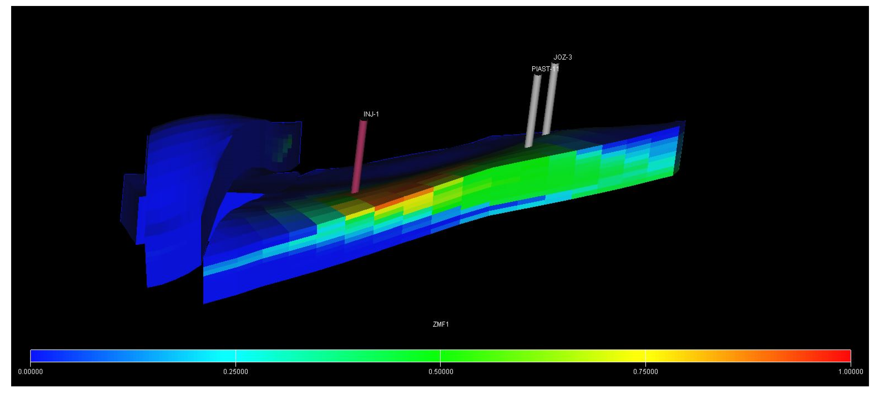
The reduction of reservoir rock oil saturation as a result of optimization of the injection wells location also directly affected the area occupied by carbon dioxide after the CCS-EOR process was completed in relation to the arbitrary scenario. The distribution of CO₂ concentration in the reservoir at the end of the CCS-EOR process for the arbitrary scenario is presented in Figure 12, and for the optimized scenario in Figure 13. In the arbitrary scenario, the places with the highest carbon dioxide concentration occur only in the immediate vicinity of the injection wells marked in red. On the other hand, optimization of the injection wells location resulted in a significant increase in the area occupied by carbon dioxide in all analyzed regions of the reservoir after the CCS-EOR process was completed in relation to the variant not including optimization. In both scenarios, the largest area with increased CO₂ concentration occurs in Region 1 due to the fact that two injection wells are located in it. However, locating an additional injection well as a result of optimization in the central part of the reservoir allowed for a significant increase in the area with a high concentration of carbon dioxide compared to the scenario in which the location was chosen arbitrarily. A similar effect was obtained for Region 2 by placing the well in the area initially occupied by gas. The optimization caused that the injection well in Region 3 was located close to the reservoir boundary due to the distribution of reservoir rock properties. The location of the well in this non-trivial place allowed for an increase in oil production, which confirms the legitimacy of using the proposed optimization algorithm. The carbon dioxide distribution in the reservoir at the end of the CCS-EOR process in individual regions is presented in Figure 14, Figure 15 and Figure 16. In all the analyzed regions, carbon dioxide moves to the upper parts of the reservoir rock due to its low specific gravity.

For the final comparison of the considered scenarios of the CCS-EOR process implementation, the net present value (NPV) was calculated for each of them. It was assumed that throughout the entire CCS-EOR process carbon dioxide obtained from the emitter is a profit because the emitter wants to utilize the produced CO₂ and pays for its collection. In addition, the costs of the produced mixture of gases injection and income from oil production were also included. In addition, before implementing the CO₂-EOR method, drilling of three injection wells was required, hence their costs were also taken into account. Fixed field operation costs and costs related to, e.g., the construction of a carbon dioxide transporting installation were omitted because they are equal in both analyzed scenarios. Thus, in this work, NPV was calculated according to the following formula [41]:

$$NPV=-C_0+{\displaystyle \sum }_{t=1}^{T_{cu}}\frac{C_t}{{\left(1+r_d\right)}^t}$$

(7)

where $NPV$ is the net present value of the project, $C_0$ is the initial investment (injection wells drilling cost), $t$ is the time step, $T_{cu}$ is the cumulative time, $C_t$ is the period cash inflow and $r_d$ is the discount rate. The total cash inflow is express in this paper as:

$$C=C_P·O+C_E·E-C_I·I$$

(8)

where $C$ is the total cash inflow, $C_P$ is the oil production income (oil price), $O$ is the produced amount of oil, $C_E$ is the revenue from CO₂ delivered from the emitter, $E$ is the amount of carbon dioxide supplied from the emitter, $C_I$ is the produced mixture of gases (CO₂ and natural gas) injection cost and $I$ is the amount of injected mixture of gases (CO₂ and natural gas).

The values of variables taken into account when calculating NPV do not change during the production time and are presented in

Table 4. Variables included in the calculation of NPV.

Variable	Value
Injection well drilling cost ($)	11,250,000
Oil production income ($/m3)	300
Revenue from CO2 delivered from the emitter ($/1000 m3)	10
Produced mixture of gases (CO2 and natural gas) injection cost ($/1000 m3)	15
Discount rate (/)	0.08

.

NPV changes over time for the considered scenarios are presented in Figure 17. The costs associated with the implementation of the CCS-EOR method cause that, in both scenarios, the NPV is initially negative. However, the increased oil production and revenues associated with receiving carbon dioxide from the emitter result in a significant increase in NPV in subsequent years of the CO₂-EOR process. This increase is slower during the CCS period, as oil is no longer produced. For the scenario in which the wells locations were chosen arbitrarily, the total revenue was $67,000,000. However, for the scenario where the optimization algorithm was applied, the CO₂-EOR phase lasts longer, generating greater profits. As a result, the total income is much larger than in the case of the arbitrary scenario and equal to $105,000,000. Therefore, the optimization enabled not only increasing the CO₂ storage capacity, which translates into a positive environmental effect, but also increases the profits associated with the implementation of the process without incurring additional investment costs relative to the scenario with the arbitrary selection of injection well locations.

7. Discussion and Conclusions

In this paper, a new algorithm to optimize the location of wells injecting carbon dioxide into the oil reservoir in order to maximize the recovery factor, which directly translates into the maximization of storage capacity for CO₂, is developed. The created method takes into account two key parameters characterizing the reservoir properties, i.e., porosity and permeability. In addition, it was checked which of these parameters had a greater impact on the selection of the optimal location of the CO₂ injection wells.

The developed optimization procedure was tested on an exemplary oil reservoir simulation model. The determined well coordinates were taken into account in the production forecast assuming the implementation of the optimized CCS-EOR process on the analyzed oil reservoir. The obtained results were compared with the option of arbitrary selection of injection wells locations based on literature analysis and preliminary computer simulations.

As a result of the injection wells location optimization, a 30% increase in oil production during the CO₂-EOR process, thus a significant increase in CO₂ storage capacity, was obtained compared to the scenario assuming arbitrary selection of injection well locations. Increased oil production from the reservoir translated into a significant reduction in reservoir rock oil saturation through which a larger area of the reservoir has been made available for carbon dioxide storage in the CCS phase. In addition, optimization of the injection wells location resulted in a significant increase in the area occupied by carbon dioxide after the CCS-EOR process was completed compared to the variant not including optimization. Based on the analyses, the NPV value for both considered scenarios was also calculated and compared. For the scenario applying the algorithm used to optimize the location of injection wells, NPV value amounted to $105,000,000. This value is almost twice as high as in the scenario in which injection wells were chosen arbitrarily.

Based on the obtained results, it can be seen that optimization of injection wells locations with the application of the created procedure enables not only an increase in CO₂ storage capacity, which translates into a positive environmental effect but also increases the profits associated with the implementation of the CCS-EOR process. It confirms both the legitimacy of using well location optimization and the effectiveness of the developed optimization method.

Compared to other well locations optimization methods, the proposed solution is more reliable because it is based on the analytical solution taking into account the most important parameters characterizing the reservoir properties, i.e., porosity and permeability. The biggest advantage over gradient optimization methods which only work in solving problems where the objective function is unimodal is the fact that in the proposed method the reservoir simulation is run not only for the best location selected from the entire reservoir but for the best location in each “mini region” what increases the probability of finding the optimal location of the injection well. On the other hand, it also outperforms gradientless optimization methods such as population algorithms that perform thousands of simulations because the created procedure reduces the number of simulations performed by omitting repeated sets of solutions, which significantly speeds up the algorithm’s execution time.

What is more, the created algorithm can also be easily adapted to fields with different geological settings because it assumes limitation of the search area to the region where only the oil phase occurs and division of this area into a given number of equal parts, which increases the probability of finding the optimal solution regardless of the geological structure of the reservoir. In addition, in the created procedure, porosity and permeability values are normalized and their weighted average is computed for further considerations and different weight ratios are checked as well what enables finding the optimal location of the CO₂ injection wells even in the case of reservoirs with difficult reservoir conditions. The proposed optimization algorithm also copes well with different production settings, because the final solution is selected based on the results of the numerical reservoir simulations carried out for all porosity and permeability weight ratios, and such coordinates are finally selected for which the location of the injection well guarantees obtaining the largest production of crude oil during the CO₂-EOR process, maximizing CO₂ storage capacity.

Taking into account the advantages of the proposed solution, it can be concluded that the developed optimization procedure can be used as a helpful tool in optimizing the location of CO₂ injection wells on the real oil fields where the CCS-EOR process is designed.