Abstract
The expected growth of the number of electric vehicles can be challenging for planning and operating power systems. In this sense, distribution networks are considered the Achilles’ heel of the process of adapting current power systems for a high presence of electric vehicles. This paper aims at deciding the maximum number of three-phase high-power charging points that can be installed in a low-voltage residential distribution grid. In order to increase the number of installed charging points, a mixed-integer formulation is proposed to model the provision of decentralized voltage support by electric vehicle chargers. This formulation is afterwards integrated into a modified AC optimal power flow formulation to characterize the steady-state operation of the distribution network during a given planning horizon. The performance of the proposed formulations have been tested in a case study based on the distribution network of La Graciosa island in Spain.
1. Introduction
A massive presence of electric vehicles may endanger the operation of distribution systems [1]. If a large number of electric vehicles is charged in a non-coordinated manner, undervoltage phenomena can happen, jeopardizing the stability of the distribution networks, [2]. In order to avoid this situation, different actions can be implemented. The easiest, but most aggressive manner to protect the distribution network operation, is to curtail the active power demand consumed by electricity end users when the normal operation of distribution networks is at danger. To prevent from this drastic measure, a wide number of smart charging procedures able to reduce the simultaneous charge of electric vehicles have been proposed during recent years [3,4]. Usually, these types of procedures need the presence of a central operator in charge of deciding at which time each electric vehicle may be charged or not. These procedures reduce the control of electric vehicle users over the initiation, duration and completion of the charging processes of their vehicles.
An alternative procedure to avoid undervoltage episodes consists in applying reactive power control mechanisms in the charging points of electric vehicles. Observe that the high resistance–reactance ratio in low-voltage distribution networks makes the reactive power support an effective tool for voltage management [5]. Traditionally, the voltage control is performed locally by injecting reactive power in those buses with voltage deviations. In this sense, the power rectifiers used in the charging points of electric vehicles are suitable to be upgraded to provide such a service [6,7]. Then, electric vehicle chargers may monitor locally the voltage at the charging point and provide the appropriate reactive power value based on a pre-established control law. Observe that this voltage control mechanism is totally decentralized and it is not required to change the charging preferences of electric vehicle users.
The active participation of electric vehicles in the operation of power systems has been extensively studied during recent years. The authors of [8] propose a number of electric vehicle charging algorithms considering explicitly the possible negative impacts on the transmission and distribution grids. A coordinated dispatch strategy for electric vehicles and renewable units at distribution level is provided in [9]. Reference [10] develops a probabilistic approach to assess the impact of electric vehicles on distribution grids considering a detailed modeling of the batteries. In reference [11], the provision of ancillary services by electric vehicles in a realistic case study is analyzed in detail. References [12,13] study the contribution of electric vehicles to the primary frequency response. Reference [14] presents a Markov decision problem that seeks to minimize the charging cost of a single electric vehicle that participates in the secondary frequency regulation. References [15,16] propose different charging procedures to minimize power losses.
The optimal planning of electric vehicle charging infrastructures has been a major concern of researchers [17]. The maximization of the penetration of electric vehicles has been studied in [18,19]. Considering that the power demanded by the charging points of electrical vehicles is quite high compared to typical consumption profiles of households, how to decide the placement of charging stations in the distribution grids is a relevant problem to solve by distribution network operators. Different approaches have been proposed to decide the optimal location of charging stations according to the needs of electric vehicle users and the particular design of distribution networks. For instance, reference [20] assumes the role of a distribution network planner aiming at expanding optimally the distribution network considering the presence of charging stations. The objective function of this problem seeks the minimization of investment and operation costs, and the maximization of the utilization of charging stations and the reliability of the distribution network. Reference [21] proposes a multi-year expansion procedure for distribution networks considering uncontrolled and smart charging. The authors of [22] propose a three-layered decision approach for deciding the location, capacity and operation policy of charging stations. Reference [23] takes the perspective of a private investor of charging stations and proposes a bi-level optimization model to maximize the expected profit obtained by the investor ensuring a certain degree of satisfaction of electric vehicle users. The optimal location of charging stations is formulated as a mixed-integer linear programming problem in [24]. In this work, the electricity demanded by electric vehicles is characterized using a novel capacitated-flow refueling location model. Finally, reference [25] proposes a capacity planning model of charging stations enforcing explicitly the reliable operation of the distribution network and the satisfaction of electric vehicle users in terms of accessibility to the charging services.
The provision of voltage support in distribution networks by electric vehicles has been also analyzed in the technical literature. Reference [26] studies different voltage support functions for electric vehicles in distribution grids with high electric vehicle penetration. The authors of [27] analyze the influence of reactive power support of electric vehicle chargers in low-voltage residential distribution grids. Reference [28] proposes a combined control scheme to improve the voltage profile in residential distribution networks considering battery storages and electric vehicles. A bidirectional charging control strategy of electric vehicles to simultaneously regulate the voltage and frequency has been developed in [29]. Reference [30] analyzes the reactive power support by electric vehicle charging stations. The authors of [31] study the capability and cost of providing reactive power service by electric vehicles. Different procedures are developed in [32] for managing the active and reactive power dispatch of a set of electric vehicles. Finally, reference [33] carries out a literature review of mathematical procedures for designing reactive power compensation in distribution networks.
This paper aims at deciding the maximum number of three-phase high-power charging points that can be installed in a low-voltage residential distribution grid. As stated in the European Roadmap on the Electrification of Road Transport [34], optimization tools are required to optimize the location of charging points and the development of the electricity network. It is assumed that the distribution network operator has to decide the maximum number of charging points that can be installed from a list of charging point requests ensuring a reliable operation of the network. We assume that charging points are private and they are installed in residential buildings. In order to increase the number of installed charging points, it is considered that charging points are able to provide reactive power support to maintain appropriate voltage levels. Unlike other mentioned works focused on the operation of distribution networks [26,27,28,29,30,31,32], the provision of reactive power support in this paper is considered from a planning perspective. Therefore, the number of charging points in the distribution network is not a known parameter, but a decision variable of the distribution network planner. Observe also that the analyzed problem is different from those focused on non-residential, large-scale charging stations [20,21,22,23,24,25]. As an example, in the case of domestic charging points, the location of charging points and the number of electric vehicles associated with each candidate charging point are know in advance. Finally, an optimal power flow problem including reactive power support constraints has been formulated in order to analyze the steady state operation of the distribution network considering the presence of new charging points.
2. Optimization Models
In this section, two optimization models are presented considering that electric vehicle chargers can provide voltage support by means of a reactive power-voltage magnitude control law. First, the mathematical formulation of this control law is provided in Section 2.1. The first optimization problem is described in Section 2.2 and intends to maximize the penetration level of electric vehicles in a given distribution network. The penetration level of electric vehicles can be defined as the maximum number of electric vehicle chargers that can be installed ensuring a reliable and secure operation of the distribution network. The second optimization model is provided in Section 2.3 and it is a modified version of the optimal power flow problem [35] that aims at simulating the operation of the distribution network considering a given number of electric vehicle chargers.
From a mathematical point of view, the formulation of the problem associated with the determination of the maximum number of charging points that can be installed in a distribution grid is challenging. The decision associated with the installation of a charging point is binary, to install or not to install, whereas the expressions modeling the power flow in the distribution network include the product of variables and trigonometric functions. As a result, the determination of the maximum number of charging points in a distribution network is a mixed-integer non-linear problem. Additionally, the modeling of voltage control by means of a reactive power-voltage droop curve is mathematically non-convex and requires the usage of additional binary variables.
The initial hypothesis and limitations of the proposed approach are the following:
- A low-voltage residential distribution network at usage is considered.
- The solution of the problem described in this work does not intend to overcome previous operation limitations of the analyzed distribution network.
- The upgrade of distribution assets is not considered. Therefore, new investments in transformers, cables, capacitors and storages are not modeled in this work.
- Since the proposed approach is focused on high-power rate chargers, only three-phase chargers are considered in this study.
- Only domestic chargers are considered. The installation of large charging stations is not taken into account in this work.
- The power factor value of electric vehicle chargers is a constant value.
- The proposed approach does not consider the coordinated charge of electric vehicles and vehicle-to-grid capability.
Since an existing residential distribution network that operates properly under normal conditions is analyzed, and three-phase chargers do not cause additional unbalances between phases, a single-phase equivalent analysis has been adopted in this paper. Observe that single-phase equivalents are typically used in planning models. However, if desired, the proposed procedure can be straightforwardly modified to incorporate a three-phase modeling of the distribution network.
Considering that the focus of this paper is to consider reactive power support by electric vehicle chargers, investments in capacity banks or storages are not included in the proposed approach. However, observe that the inclusion of capacity banks, lines upgrading, etc., can be easily integrated.
Finally, the notation used throughout the rest of this section is included in the Appendix A for quick reference.
2.1. Reactive Power—Voltage Magnitude Control Law Formulation
Since distribution networks are traditionally associated with high resistance–reactance ratios, the effect of resistance is no longer negligible, and the assumptions taken for high-voltage systems are no longer valid. An effective procedure to mitigate voltage decrements is to reduce the active power consumption in the grid. This is a very effective tool, but implies the modification of the consumption patterns of electricity end-users [36]. For this reason, local reactive power injection mechanisms are typically used, since they do not need the installation of additional devices and exploit the capability of the inverters used in electric vehicle charging points.
Figure 1 represents graphically a typical reactive power-voltage magnitude control law for a given electric vehicle charger k located in bus n on day d and period t, [37]. The reactive power demanded by the charging point is denoted by , whereas the voltage magnitude is . If the nodal voltage is low, , the reactive power demanded by the charger point is a negative value, , corresponding with the maximum reactive power that can be injected by the charger into the grid. As the voltage magnitude increases, , the injection of reactive power decreases linearly. Finally, if the voltage magnitude is greater than , , the reactive power injected by the charging point is equal to zero.
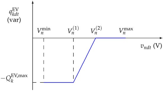
Figure 1.
Reactive power-voltage magnitude droop curve.
Symbols and denote the apparent power and the power factor of charger k, respectively. Equations (2) and (3) compute the maximum active and reactive powers associated with a charger for a given power factor, . It is assumed that the active power consumed by the charger is equal to the maximum value, but the reactive power is dependent on the nodal voltage magnitude, as defined in (1). Parameters and in Equations (4) and (5) are used to compute the reactive power injection associated with the voltage magnitude level when the voltage takes values between and , as represented in Figure 1. Observe that the reactive power in this interval is a linear expression of the voltage magnitude with intercept and slope equal to and , respectively.
Traditionally, electric vehicle chargers operate with power factor equal to 1. Therefore, if , then and . However, hereinafter it is assumed a leading power factor, , and that electric vehicle chargers are able to inject reactive power as shown in Figure 1.
Observe that expression (1) cannot be incorporated directly into the formulation of an optimization problem. The reason of this is that the mathematical expression of is a piecewise function of the optimization variable representing nodal voltage magnitudes, . The mathematical formulation of piecewise functions using mixed-integer linear expressions has been typically used in different power system problems, [38,39]. Therefore, constraints (6)–(14) are proposed to equivalently formulate (1). In this formulation, binary variables and are used to identify the block associated with the value of in the piecewise function (1). In this manner, the voltage is in the first block if ; if , the voltage is in the second block; finally, the voltage is in the third block if . For the sake of clarity, Table 1 provides the rationale of variables . In formulation (6)–(14), variable is equal to if is within block j, being equal to 0 otherwise. This equality is enforced through constraints (6)–(9). In these constraints, the values of binary variables are assigned depending on the value of . For instance, if is in the first block, it has to be satisfied that . To obtain this result, the only feasible solution is , , and . A similar reasoning can be done for blocks 2 and 3. The value of is assigned through constraints (10). If and , then , whereas if and . Note that the combination is not allowed by constraints (11). Finally, if and , is in the second block of the droop curve, , and should be expressed as . However, this expression contains the non-linear product of variables and . In order to preserve the linearity of the formulation, the auxiliary variable is used to equivalently represent the product of and . The linearization of the product of a continuous and a binary variable has been previously done, for instance, in [40]. The assignment is linearly expressed through constraints (12) and (13). In these constraints, M is a big enough parameter . If and , then constraints (12) state that and . On the other hand, if , then is either in the first or third block of the piecewise function (1) and by constraints (13). The performance of constraints (12) and (13) is described in Table 2. Finally, the binary nature of variables is stated in (14).

Table 1.
Rationale of variables .
Table 2.
Linearization of product .
2.2. Maximization of the Penetration Level of Electric Vehicles
The maximization of the penetration level of electric vehicles is formulated in this subsection. In this problem, a low-voltage distribution network operating under normal conditions is considered.
It is also assumed that the distribution network planner has a request list of high-power three-phase electric vehicles chargers that are desired to be installed in the distribution network.
Each charging point request is indexed by k and has information about the location of the charger in the distribution network and the nominal charge rate, . The objective of the distribution network planner is to accept the maximum number of charger point requests ensuring the adequate operation of the network. For doing that, the worst case is analyzed, which means that the distribution network has to be capable of operating in normal conditions assuming a simultaneity factor equal to 1. In other words, it is assumed that the distribution network has to be capable of operating under normal operation limits when households consume the contracted peak power and all electric vehicles are simultaneously charging. Note that this strong requirement can be relaxed if desired to obtain a larger penetration level of electric vehicles. Finally, note that this problem is solved by a single time period, i.e., , . The formulation of this problem is the following:
Subject to:
- Voltage magnitude limits
- Distribution transformer capacity constraints
- Active and reactive power flow constraints
- Active and reactive power balance constraints
- Reactive power—voltage magnitude control constraints
The objective function (15) represents the maximization of the number of accepted requests of electric vehicle chargers. The acceptance of a request is characterized by binary variable that is equal to 1 if charger k is accepted, being equal to zero otherwise. Voltage magnitudes are bounded by constraints (16). Constraints (17) limit the power output of each distribution transformer s. Despite the fact that distribution networks are usually operated as radial systems, for the sake of generality, we have considered in this formulation that several distribution substations may feed the analyzed residential distribution system. The active and reactive power flows through distribution lines are expressed by constraints (18) and (19), respectively. As usual, distribution lines are represented by using the series impedance model. The capacity of the lines is bounded by constraints (20). Equations (21) and (22) establish the active and reactive power balances in each bus for each time period. These equations enforce the active and reactive power balances in each bus of the distribution network considering the nodal consumption and distribution line flows. Finally, constraints (23)–(25) formulate the reactive power-voltage magnitude control law for those selected chargers. Constraints (23) and (24) are used to state that the reactive power contribution of charger k, , must be equal to if charger k is accepted (), being equal to zero if the charger is not selected (). Note that the value of depends on the nodal voltage magnitude , as formulated in (6)–(14).
2.3. Operation of the Distribution Network Considering Voltage Management of Electric Vehicles
This subsection solves an optimal power flow (OPF) problem to simulate the steady-state operation of a distribution network considering that electric vehicles can provide voltage support. This problem can be solved sequentially to simulate the operation during a planning horizon. This problem is denoted as (P2) and is formulated as follows:
- Voltage limits
- Assignment of selected charging points
where comprises all optimization variables in problem (P2) for day d and period t.
The objective function of (P2) is formulated in (26) and consists in minimizing voltage deviations over upper and lower limits, and . Since these voltage deviations are penalized in the objective function (26), they will be greater than zero only in the case in which the demand cannot be procured satisfying all the technical constraints of the distribution network. The voltage magnitude limits, including positive and negative deviations, are formulated in (27) and (28). Finally, the charging points considered in the formulation are specified through constraints (29), being the optimal values of variables obtained from solving problem (P1).
2.4. Tool Usage
The usage of the optimization models presented in this section is described below:
- Distribution network operators may determine the maximum number of charging points for electric vehicles by solving problem (P1). The most important input data needed to solve this problem are: (i) the technical data of the distribution network, (ii) the peak power contracted by each consumer, (iii) the technical characteristics of the candidate charging points, and (iv) the parameters describing the reactive power droop curve. The outputs of this problem are the set of candidate charging points that are accepted to be installed in the considered distribution network.
- The steady-state behavior of the distribution network considering reactive power injections and the set of installed charging points is characterized by solving problem (P2). This problem can be solved for a specified number of days and time periods. The input data of this problem are: (i) the technical data of the distribution network, (ii) the location and technical characteristics of each accepted charging point, (iii) the actual energy consumption per bus and period (considering electric vehicle demand), and (iv) the parameters describing the reactive power droop curve. The main outputs of this problem are (i) voltages per bus and period and (ii) active and reactive power flows per line and period.
Figure 2 represents graphically the tool usage described above:
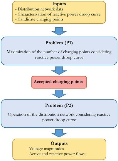
Figure 2.
Tool usage.
3. Illustrative Example
In this section we solve an illustrative example to analyze the impact of considering the reactive power-voltage magnitude droop curve in the selection process of charging points. We assumed a radial distribution network where a distribution transformer feeds the demand of four buses. As stated in Section 2, a single-phase analysis was performed in this study. Each demand bus consumed 9 kW and 1 kva per phase, and had associated a charging point request of 5 kVA per phase. The magnitudes of the impedance and resistance of each line branch were equal to 128.8 and 32.2 , respectively. The nominal single phase voltage magnitude was 230 V. The minimum and maximum values of voltage magnitudes were 0.95 and 1.05 times the nominal value, i.e., 218.5 and 241.5 V, respectively. Parameters and describing the reactive power-voltage magnitude curve were equal to 224.25 and 230 V, respectively. The power factor of the charger points in the case considering the reactive power-voltage magnitude droop curve was equal to 0.9 (leading). Therefore, 4.5 kW, whereas kvar. The capacity of the lines, , was 100 kVA. Please note, that the values of the parameters selected for this case study are not meant to be representative of a realistic network and they are only used for illustrative purposes.
The main results obtained are depicted in Figure 3 and Figure 4, respectively. These figures provide per phase values associated with voltage magnitudes, consumption of active and reactive power and number of installed charging points per bus, as well as active and reactive power flows per line. For the sake of clarity, indices d and t have been omitted from the mathematical symbols included in both figures. Figure 3 provides the results obtained from solving problem (P1) without considering the reactive power droop curve. In other words, problem (15)–(22) was solved enforcing . From Figure 3 we can conclude that the power transfer capability of the analyzed network was low and no charging points could be installed without violating voltage limits (). In this sense, we observed that the voltage magnitude in the transformer network bus was greater than the nominal value, V, whereas the voltage magnitude at the final bus, 4, was equal to the lower voltage limit, 218.5V.
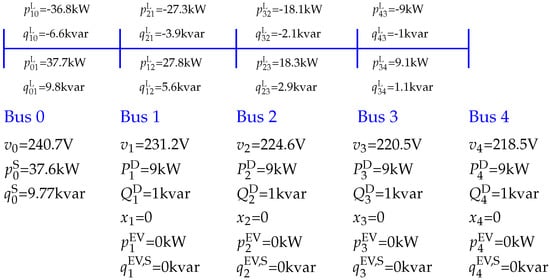
Figure 3.
Illustrative example: Results of problem (P1) without reactive power droop curve.
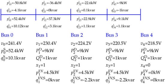
Figure 4.
Illustrative example: Results of problem (P1) with reactive power droop curve.
Figure 4 provides the obtained results when the reactive power droop curve was considered. In this case, three charging points were installed (buses 1, 2 and 3). Since the power factor of the charger was 0.9, the active power demand of each charging point was reduced from 5kW (power factor equal to 1) to 4.5 kW (power factor equal to 0.9). Besides, it is observed that reactive power was injected from the charging points into the grid if voltage magnitudes are lower than V. This was the case of buses 2 and 3, with voltage magnitudes equal to 224.2 and 220.5 V, respectively.
Table 3 provides the values of the variables and for each bus of the network in which a charging point was installed. Observe that only bus 1 had a voltage magnitude greater than , which results in and by constraints (6)–(14). On the other hand, voltages in buses 2 and 3 were lower than , which resulted in , and kvar. Observe that a negative value of indicates a reactive power injection on the bus where charger k was located (constraint (22)).
Table 3.
Illustrative example: Variables .
4. Case Study
This section analyzes a case study based on the distribution system of La Graciosa, Canary Islands, Spain. La Graciosa is a small island of 27 km with a population around 660 people [41]. This case study is focused on a district that is fed by a single 400-kVA power transformer, [42]. This district comprises 26 buildings that are connected by 26 lines.
4.1. Input Data
Figure 5 shows the location of the district and the buildings. The distribution network is represented in Figure 6.
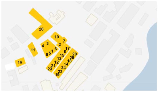
Figure 5.
Case study: Location of the distribution network.
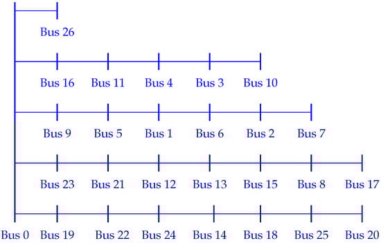
Figure 6.
Case study: Distribution network [42].
The demands associated with the considered buildings were obtained from the first 26 residential demands provided in [43], which are downloadable in [44]. In this case study we assumed that there were no charging points in the district. In order to analyze a case in which a high number of chargers are demanded, it was assumed that 44 charging points were requested, that is the number of electric vehicles associated with the first 26 households in [43]. The power factor of residential demands was equal to 0.95 (lagging).
The main input data describing the considered distribution network are provided in Table 4. All loads were assumed to have a three-phase grid connection and a nominal neutral-to-phase voltage magnitude equal to 230 V. The minimum and maximum values that voltage magnitudes could take were 0.95 and 1.05 times the nominal value, i.e., 218.5 and 241.5 V, respectively. Parameters and describing the reactive power-voltage magnitude curve were equal to 224.25 and 230 V, respectively. The power factor of the charging points in the case in which the reactive power-voltage magnitude droop curve was considered was 0.95 (leading).
Table 4.
Case study: input data.
The performances of problems (P1) and (P2) were analyzed by considering two typical three-phase chargers with rate powers equal to 11 and 22 kVA.
All mathematical cases were solved using GAMS and Dicopt 12.6.111 in a linux-based server of four 3.0 GHz processors and 250 GB of RAM. Due to the complexity of mixed-integer non-linear programs, it is convenient to solve problems (P1) and (P2) starting from a so-called warm start solution. For doing that, problems (P1) and (P2) were solved neglecting the reactive power injections (6)–(14) and binary variables and . Afterwards, initial values of variables and could be assigned as a function of the resulting voltage magnitudes in the previous problem. Therefore, for the warm start solution, if , then ; if , then ; and , then .
4.2. Results: Maximization of Number of Charging Points
This section analyzes the performance of problem (P1) on the distribution network described above. In order to analyze the advantages of considering the reactive power-voltage magnitude droop curve, all cases have been also solved without considering the reactive power droop curve. Besides, with the aim of analyzing the influence of the distribution line parameters, two different sets of data were used to characterize the distribution lines, namely and . In , it was assumed that the impedance of each line was equal to 0.551 + 0.089i [27], whereas it was equal to 0.716 + 0.089i for . Observe that the relationship resistance/reactance of was equal to 6.1, whereas it was equal to 8.6 for . Observe that high resistance/reactance ratios were typical of low-voltage distribution networks. Considering the values of the impedances in cases and , the power transfer capability of the network would be higher for than for . In this manner, it was expected that the voltage droop along the lines in case would be higher than that in case .
Table 5 provides the results obtained from solving problem (P1) in terms of the number of charging points and the voltage magnitude in each bus of the system for each case. In total, eight different cases have been solved in this section. The average number of constraints, continuous and binary variables was equal to 734, 191 and 93, respectively. Each case was solved in a time smaller than 0.2 s. From the results provided in Table 5 we can observe that the number of charging points resulting from the model considering the reactive power droop curve was always greater than those obtained in the case without reactive power droop curve. If reactive power injections were considered, the number of installed charging points were up to 8.3% and 10.7% higher for 11 and 22 kVA chargers, respectively. As expected, the number of installed charging points strongly depended on the nominal power of the charger (11/22 kVA) and on the parameters of the lines (, ). Focusing on the model with reactive power droop curve and , we observed that the number of charging points decreased from 26, for a 11 kVA charger, to 21, for a 22 kVA charger. For , the number of installed charging points was lower and it was equal to 21 for a 11 kVA charger, and 15 for a 22 kVA charger. It was also observed that the voltage magnitudes at some ending buses (7, 17 and 20) were close to the minimum allowed voltage magnitude, 218.5 V. These voltage values indicated that the installation of additional charging points in these lines was not feasible.
Table 5.
Case study: Selection of charging points and voltage magnitudes.
4.3. 30-Days Simulation
In this subsection we solve problem (P2) to analyze the steady-state operation of the distribution network during a planning horizon of 30 days divided into 10-min periods. For doing that, we simulate the operation of the distribution network considering 11 and 22 kVA chargers using the distribution line parameters denoted by . The aggregated hourly demand is depicted in Figure 7.
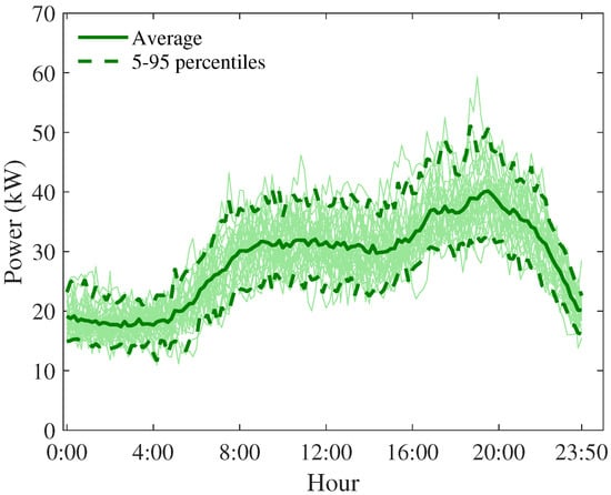
Figure 7.
Case study: aggregated residential demand.
The energy charged in each 10-min period by each electric vehicle was generated from the charging profile L1 included in [43]. Based on these data, the daily energy charged and the starting hour of the charging for each electric vehicle were characterized as random variables. Therefore, a Kernel density distribution has been fitted for each random variable and for each electric vehicle, as done in [45]. The resulting daily probability distributions for each of the 41 electric vehicles are represented in Figure 8. Figure 8a indicates that the average daily energy charged per vehicle was less than 10 kWh, whereas Figure 8b shows that the charge of the vehicles usually started in the middle part of the day.
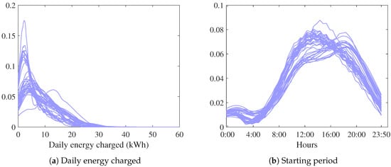
Figure 8.
Case study: probability distributions of the daily energy charged and the starting hour of the charging per vehicle.
Using the probability distributions represented in Figure 8, different charging profiles have been randomly generated for each day considering 11 and 22 kVA chargers and 10-min time periods. In order to analyze the influence of increasing the charging demand of electric vehicles, two additional cases were generated considering that the energy demanded by the electric vehicles was 50% higher. The cases generated from the energy values represented in Figure 8a are denoted by 11 kVA- and 22 kVA-, whereas cases with higher energy demanded are denoted by 11 kVA- and 22 kVA-, respectively. As an example, the average energy charged per vehicle and day in case 11 kVA- was 8.5 kWh resulting, for a typical electric vehicle consumption rate of 0.2 kWh/km, in a daily distance driven equal to 42.5 km. The resulting charging profiles are provided in Figure 9.
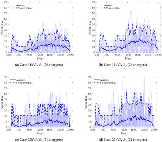
Figure 9.
Case study: aggregated charging profiles.
Because of the variation of the demand during the day, three different voltage levels were considered in the distribution transformer bus in order to provide voltage support: 231 V from 0:00 to 6:00 h and from 23:00 to 23:50 h; 232 V from 17:00 to 21:00 h; and 231.5 V for the rest of hours.
Considering cases with and without reactive power provision, a total number of instances of problem (P2) have been solved in this section. The average number of constraints, continuous and binary variables was equal to 734, 245 and 34, respectively. Each single instance was solved in a time smaller than 0.02 s.
Table 6 provides the minimum () and mean () voltage magnitudes and the sum of the reactive power injected () per bus and case during the 30-day simulation. It was verified that voltage magnitudes were always greater than the lower limit, 218.5 V, and none voltage violations have been observed in the analyzed cases. As expected, voltage magnitudes were lower in those buses that were located furthest from the distribution transformer. In general, voltages decreased as the rate power of the charger and the energy charged increased. However, it was noticed that effect of increasing the power of the charger was more relevant than the growth of the energy demanded. For instance, from case 11kVA- to case 22kVA-, the average minimum voltage decreased 0.3 V, whereas this difference was 0.2 V if cases 11 kVA- and 11 kVA- were compared.
Table 6.
Case study: voltage magnitudes per bus (V) and reactive power injections (kvarh).
Table 6 shows that the reactive power injected was higher in those chargers located far from the distribution transformer. In this sense, the reactive power injected in the closest buses to the transformer (buses 9, 19, 23 and 26) is always 0. Additionally, the injection of reactive power grew as the rate power of the charger and the energy charged increased. For instance, a total amount of 382.8 kvarh was injected into the grid in case 11 kVA-. This value corresponded to an average value of 14.7 kvarh per charger. This value increased 25.2% and 56.1% in cases 22 kVA- and 11kVA-, respectively.
As an example, Figure 10 represents the results obtained for bus 10 during the first day in case 11kVA- in terms of voltage magnitudes, active power consumed by the household and the electric vehicles, and the injected reactive power. As indicated in Table 5, two electric vehicles chargers were installed in bus 10. As observed in Figure 10c, one vehicle started the charging at 8:10 am, and the other at 11:40 am. The total energy consumed by the house, without considering electric vehicles, was 8.9 kWh, whereas the sum of the energy charged by two electric vehicles was only 3.5 kWh. However, the highest active power peaks corresponded to the periods in which the vehicles were being charged. The high active power demanded by the electric vehicle chargers had a high impact on voltage magnitudes. Figure 10a shows that voltage drops occurred when electric vehicles were charging. Since voltages were under the nominal value, 230 V, reactive power was injected into the grid, as observed in Figure 10d. Finally, Figure 10b shows that the voltage magnitudes in the case in which the reactive power droop was considered are higher than those in the case in which the reactive power droop was not accounted for.
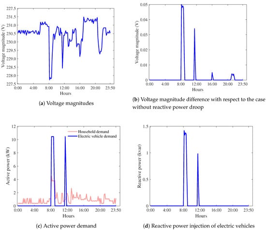
Figure 10.
Case study: Results bus 10 (11 kVA-).
Finally, Figure 11 represents the average values and difference between voltage magnitudes in cases 11 kVA- and 22 kVA- using models with and without reactive power injection. For the sake of conciseness, a set of selected buses corresponding with the last buses of each branch were considered. The positive values of this difference indicated that voltages in cases with reactive power injection were higher than those in cases without reactive power injection. It was observed that the average voltage difference was larger in those periods with higher demand (between 12 and 22 h).
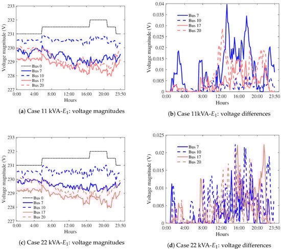
Figure 11.
Case study: comparison of voltage magnitudes.
5. Conclusions
This paper has presented a non-linear mixed-integer formulation for deciding the maximum number of charging points of electric vehicles that can be installed in a low-voltage distribution network. In order to increase the number of charging points, it has been considered that charging points are able to provide voltage support by injecting reactive power if voltage magnitudes are lower than a specified value. Therefore, the reactive power-voltage magnitude control is activated locally and it does not require the presence of a central operator. Additionally, an optimal power flow formulation has been provided to simulate the steady-state operation of a distribution network considering that electric vehicles can provide voltage support.
The proposed model is tested on a case study based on La Graciosa distribution network. Based on the numerical results presented in the case study, it has been observed that the number of installed charging points is higher if reactive power injections are considered. These increases are up to 8.3% and 10.7% for 11 and 22 kVA chargers, respectively. It has been also observed that the parameters of the distribution lines have a high influence on the number of installed chargers. For instance, if the resistance of the lines decreases 50%, the number of installed chargers increases 19.2% and 21.0% for 11 and 22 kVA chargers, respectively. It has been verified through 30-day simulations that the voltage magnitudes resulting from the model including reactive power injections are greater than the specified lower voltage limit. It has been also observed that the effect of increasing the power of the charger is more relevant than the growth of the energy demanded in terms of voltage decrease.
Research is currently underway to optimize the power factor assigned to each charger in order to maximize the number of installed charging points.
Author Contributions
M.C. proposed the core idea, performed the simulations and exported the results. M.C., R.Z.-M. and R.D. contributed to the design of the models and the writing of this manuscript. All authors have read and agreed to the published version of the manuscript.
Funding
This work has been supported by the Ministry of Economy and Competitiveness of Spain under Project DPI2015-71280-R MINECO/FEDER, UE and by the Ministry of Science and Innovation of Spain under Project PID2019-111211RB-I00/AEI/10.13039/501100011033.
Acknowledgments
The authors of this work would like to acknowledge and dedicate this paper to Spanish health professionals that have put their lives at risk and worked hard against COVID-19 while this paper was written.
Conflicts of Interest
The authors declare no conflict of interest.
Appendix A. Notation
The notation used throughout the paper is included below for quick reference. Observe that the definitions of symbols included in this appendix pretend to be general enough to be used in the two optimization models formulated in this paper. Unless otherwise indicated, all symbols refer to per-phase values.
Sets and Indices
- D
- Set of days, indexed by d
- K
- Set of electric vehicle chargers, indexed by k
- Set of electric vehicles chargers at usage in bus n, day d and period t.
- L
- Set of distribution lines
- N
- Set of buses, indexed by n and m
- Set buses connected to bus n, indexed by n and m
- S
- Set of distribution transformers, indexed by s
- Set of distribution transformers in bus n, indexed by s
- T
- Set of time periods, indexed by t
Parameters
- Susceptance of the line linking buses n and m
- Conductance of the line linking buses n and m
- M
- Large enough parameter
- Active power demand in bus n, day d and period t
- Active power demanded by charger k on day d and period t
- Active power rate of charger k
- Reactive power demand in bus n, day d and period t
- Maximum reactive power that can be consumed by charger k
- Reactive power consumed by charger k on day d and period t
- Rate charge power of charger k
- Capacity of the line linking buses n and m
- Capacity of distribution transformer s
- First breakpoint of the reactive power-voltage magnitude droop curve of bus n
- Second breakpoint of the reactive power-voltage magnitude droop curve of bus n
- Upper limit of the voltage magnitude of bus n
- Lower limit of the voltage magnitude of bus n
- Auxiliary parameter used to formulate the reactive power-voltage magnitude droop curve of charger k in bus n
- Auxiliary parameter used to formulate the reactive power-voltage magnitude droop curve of charger k in bus n
- Power factor angle of charger k
Variables
- Active power flow through line linking buses n and m on day d and period t
- Active power supplied by distribution transformer s on day d and period t
- Reactive power that must be consumed by charger k on day d and period t, if the charging point is accepted
- Reactive power consumed by charger k on day d and period t
- Reactive power flow through line linking buses n and m on day d and period t
- Reactive power supplied by distribution transformer s on day d and period t
- Voltage magnitude of bus n on day d and period t
- Positive voltage magnitude deviation in bus n on day d and period t
- Negative voltage magnitude deviation in bus n on day d and period t
- Auxiliary continuous variable used to linearize the bilinear product of variables and
- Auxiliary continuous variable associated with block-j of the voltage magnitude of bus n on day d and period t
- Binary variable that is equal to 1 if the request for charging point k is accepted
- Auxiliary binary variable used to formulate the reactive power-voltage magnitude droop curve of bus n on day d and period t
- Auxiliary binary variable used to formulate the reactive power-voltage magnitude droop curve of bus n on day d and period t
- Voltage angle of bus n on day d and period t
References
- Melhorn, A.C.; McKenna, K.; Keane, A.; Flynn, D.; Dimitrovski, A. Autonomous plug and play electric vehicle charging scenarios including reactive power provision: A probabilistic load flow analysis. IET Gener. Transm. Distrib. 2017, 11, 768–775. [Google Scholar] [CrossRef]
- Graham, R.L.; Francis, J.; Bogacz, R.J. Challenges and Opportunities of Grid Modernization and Electric Transportation; U.S. Department of Energy: Washington DC, USA, 2017.
- Knezović, K.; Marinelli, M.; Zecchino, A.; Andersen, P.B.; Traeholt, C. Supporting involvement of electric vehicles in distribution grids: Lowering the barriers for a proactive integration. Energy 2017, 134, 458–468. [Google Scholar] [CrossRef]
- Arias, N.B.; Hashemi, S. Distribution System Services Provided by Electric Vehicles: Recent Status, Challenges, and Future Prospects. IEEE Trans. Intell. Transp. Syst. 2019, 20, 4277–4296. [Google Scholar] [CrossRef]
- Gómez Expósito, A.; Conejo, A.J.; Cañizares, C. (Eds.) Electric Energy Systems: Analysis and Operation; The Electric Power Engineering Series; CRC Press: Boca Raton, FL, USA, 2009. [Google Scholar]
- Demirok, E.; Casado-González, P.; Frederiksen, K.H.; Sera, D.; Rodríguez, P.; Teodorescu, R. Local reactive power control methods for overvoltage prevention of distributed solar inverters in low-voltage grids. IEEE J. Photovolt. 2011, 1, 174–182. [Google Scholar] [CrossRef]
- Sortomme, E.; Negash, A.I.; Venkata, S.S.; Kirschen, D.S. Voltage dependent load models of charging electric vehicles. In Proceedings of the IEEE PES General Meeting, Vancouver, BC, Canada, 21–25 July 2013; pp. 1–5. [Google Scholar]
- Munoz, E.R.; Razeghi, G.; Zhang, L.; Jabbari, F. Electric vehicle charging algorithms for coordination of the grid and distribution transformer levels. Energy 2016, 113, 930–942. [Google Scholar] [CrossRef]
- Wang, L.; Sharkh, S.; Chipperfield, A. Optimal coordination of vehicle-to-grid batteries and renewable generators in a distribution system. Energy 2016, 113, 1250–1264. [Google Scholar] [CrossRef]
- Valsera-Naranjo, E.; Sumper, A.; Villafafila-Robles, R.; Martínez-Vicente, D. Probabilistic Method to Assess the Impact of Charging of Electric Vehicles on Distribution Grids. Energies 2012, 1503–1531. [Google Scholar] [CrossRef]
- Ciechanowicz, D.; Knoll, A.; Osswald, P.; Pelzer, D. Towards a business case for vehicle-to-Grid: Maximizing profits in ancillary service markets. In Plug in Electric Vehicles in Smart Grids. Power Systems; Rajakaruna, S., Shahnia, F., Ghosh, A., Eds.; Springer: Singapore, 2015. [Google Scholar]
- Mu, Y.; Wu, J.; Ekanayake, J.; Jenkins, N.; Jia, H. Primary frequency response from electric vehicles in the Great Britain power system. IEEE Trans. Smart Grid 2013, 4, 1142–1150. [Google Scholar] [CrossRef]
- Carrión, M.; Domínguez, R.; Cañas-Carretón, M.; Zárate-Miñano, R. Scheduling isolated power systems considering electric vehicles and primary frequency response. Energy 2019, 168, 1192–1207. [Google Scholar] [CrossRef]
- Donadee, J.; Ilic, M.D. Stochastic optimization of grid to vehicle frequency regulation capacity bids. IEEE Trans. Smart Grid 2014, 5, 1061–1069. [Google Scholar] [CrossRef]
- Clement-Nyns, K.; Driesen, J. The impact of charging plug-in hybrid electric vehicles on a residential distribution grid. IEEE Trans. Power Syst. 2010, 25, 371–380. [Google Scholar] [CrossRef]
- Sortomme, E.; Hindi, M.M.; MacPherson, S.D.J.; Venkata, S.S. Coordinated charging of plug-in hybrid electric vehicles to minimize distribution system losses. IEEE Trans. Smart Grid 2011, 2, 198–205. [Google Scholar] [CrossRef]
- Abdalrahman, A.; Zhuang, W. A Survey on PEV Charging Infrastructure: Impact Assessment and Planning. Energies 2017, 10, 1650. [Google Scholar] [CrossRef]
- Humayd, A.S.B.; Bhattacharya, K. A Novel Framework for Evaluating Maximum PEV Penetration into Distribution Systems. IEEE Trans. Smart Grid 2018, 9, 2741–2751. [Google Scholar] [CrossRef]
- Zárate-Miñano, R.; Flores Burgos, A.; Carrión, M. Analysis of different modeling approaches for integration studies of plug-in electric vehicles. Int. J. Electr. Power Energy Syst. 2020, 114, 105398. [Google Scholar] [CrossRef]
- Xiang, Y.; Yang, W.; Liu, J.; Li, F. Multi-objective distribution network expansion incorporating electric vehicle charging stations. Energies 2016, 9, 909. [Google Scholar] [CrossRef]
- Zeng, B.; Feng, J.; Zhang, J.; Liu, Z. An optimal integrated planning method for supporting growing penetration of electric vehicles in distribution systems. Energy 2017, 126, 273–284. [Google Scholar] [CrossRef]
- Kong, C.; Jovanovic, R.; Bayram, I.S.; Devetsikiotis, M. A hierarchical optimization model for a network of electric vehicle charging stations. Energies 2017, 10, 675. [Google Scholar] [CrossRef]
- Liu, Y.; Xiang, Y.; Tan, Y.; Wang, B.; Liu, J.; Yang, Z. Optimal Allocation Model for EV Charging Stations Coordinating Investor and User Benefits. IEEE Access 2018, 6, 36039–36049. [Google Scholar] [CrossRef]
- Zhang, H.; Moura, S.J.; Hu, Z.; Song, Y. PEV Fast-Charging Station Siting and Sizing on Coupled Transportation and Power Networks. IEEE Trans. Smart Grid 2018, 9, 2595–2605. [Google Scholar] [CrossRef]
- Abdalrahman, A.; Zhuang, W. QoS-Aware Capacity Planning of Networked PEV Charging Infrastructure. IEEE Open J. Veh. Technol. 2020, 1, 116–129. [Google Scholar] [CrossRef]
- Huang, S.; Pillai, J.R.; Bak-Jensen, B.; Thøgersen, P. Voltage support from electric vehicles in distribution grid. In Proceedings of the 15th European Conference on Power Electronics and Applications (EPE), Lille, France, 2–6 September 2013; pp. 1–8. [Google Scholar]
- Leemput, N.; Geth, F.; Van Roy, J.; Büscher, J.; Driesen, J. Reactive power support in residential LV distribution grids through electric vehicle charging. Sustain. Energy Grids Netw. 2015, 3, 24–35. [Google Scholar] [CrossRef]
- Behravesh, V.; Keypour, R.; Akbari Foroud, A. Control strategy for improving voltage quality in residential power distribution network consisting of roof-top photovoltaic-wind hybrid systems, battery storage and electric vehicles. Sol. Energy 2019, 182, 80–95. [Google Scholar] [CrossRef]
- Mohammadi, F.; Nazri, G.-A.; Saif, M. A Bidirectional Power Charging Control Strategy for Plug-in Hybrid Electric Vehicles. Sustainability 2019, 11, 4317. [Google Scholar] [CrossRef]
- Kesler, M.; Kisacikoglu, M.C.; Tolbert, L.M. Vehicle-to-grid reactive power operation using plug-in electric vehicle bidirectional offboard charger. IEEE Trans. Ind. Electron. 2014, 61, 6778–6784. [Google Scholar] [CrossRef]
- Mojdehi, M.N.; Fardad, M.; Ghosh, P. Technical and economical evaluation of reactive power service from aggregated EVs. Electr. Power Syst. Res. 2016, 133, 132–141. [Google Scholar] [CrossRef]
- Wang, J.; Bharati, G.R.; Paudyal, S.; Ceylan, O.; Bhattarai, B.P.; Myers, K.S. Coordinated electric vehicle charging with reactive power support to distribution grids. IEEE Trans. Ind. Informat. 2018, 15, 54–63. [Google Scholar] [CrossRef]
- Stanelyte, D.; Radziukynas, V. Review of Voltage and Reactive Power Control Algorithms in Electrical Distribution Networks. Energies 2020, 13, 58. [Google Scholar] [CrossRef]
- ERTRAC; EPoSS; ETIP SNET. European Roadmap Electrification of Road Transport. 2017. Available online: https://egvi.eu/wp_content/uploads/2018/01/ertrac_electrificationroadmap2017.pdf (accessed on 5 July 2020).
- Carpentier, J. Contribution to the economic dispatch problem. Bull. Soc. Fr. Electr. 1962, 8, 431–447. [Google Scholar]
- Yang, G.; Marra, F.; Juamperez, M.; Kjaer, S.B.; Hashemi, S.; Østergaard, J.; Ipsen, H.H.; Frederiksen, K.H. Voltage rise mitigation for solar PV integration at LV grids. J. Mod. Power Syst. Clean Energy 2015, 3, 411–421. [Google Scholar] [CrossRef]
- Pukhrem, S.; Basu, M.; Conlon, M.F.; Sunderland, K. Enhanced network voltage management techniques under the proliferation of rooftop solar PV installation in low-voltage distribution network. IEEE J. Emerg. Sel. Top. Power Electron. 2017, 5, 681–694. [Google Scholar] [CrossRef]
- Arroyo, J.M.; Conejo, A.J. Optimal response of a thermal unit to an electricity spot market. IEEE Trans. Power Syst. 2000, 15, 1098–1104. [Google Scholar] [CrossRef]
- Conejo, A.J.; Arroyo, J.M.; Contreras, J.; Villamor, F.A. Self-scheduling of a hydro producer in a pool-based electricity market. IEEE Trans. Power Syst. 2002, 17, 1265–1271. [Google Scholar] [CrossRef]
- Carrión, M.; Dvorkin, Y.; Pandžić, H. Primary Frequency Response in Capacity Expansion with Energy Storage. IEEE Trans. Power Syst. 2018, 33, 1824–1835. [Google Scholar] [CrossRef]
- Asensio, M.; Meneses de Quevedo, P.; Muñoz-Delgado, G.; Contreras, J. Joint Distribution Network and Renewable Energy Expansion Planning considering Demand Response and Energy Storage—Part II: Numerical Results. IEEE Trans. Smart Grid 2018, 9, 667–675. [Google Scholar] [CrossRef]
- Sánchez, J.; Pavón, M.C.; Romero, L.; Guerrero, M.C.; Álvarez, S. Potential for exploiting the synergies between buildings through DSM approaches. Case study: La Graciosa Island. Energy Convers. Manag. 2019, 194, 199–216. [Google Scholar] [CrossRef]
- Muratori, M. Impact of uncoordinated plug-in electric vehicles charging on residential power demand. Nat. Energy 2018, 3, 193–201. [Google Scholar] [CrossRef]
- Muratori, M. Impact of Uncoordinated Plug-in Electric Vehicle Charging on Residential Power Demand—Supplementary Data. Available online: https://data.nrel.gov/submissions/69 (accessed on 25 May 2020).
- Carrión, M. Determination of the selling price offered by electricity suppliers to electric vehicle users. IEEE Trans. Smart Grids 2019, 10, 6655–6666. [Google Scholar] [CrossRef]


© 2020 by the authors. Licensee MDPI, Basel, Switzerland. This article is an open access article distributed under the terms and conditions of the Creative Commons Attribution (CC BY) license (http://creativecommons.org/licenses/by/4.0/).