Mathematical Model of a Sun-Tracked Parabolic Trough Collector and Its Verification

Abstract

The paper presents a one-dimensional distributed parameter model for simulating the transient-state operation of a parabolic trough collector (PTC). The analyzed solar collector has a module design and is equipped with a two-axis sun-tracking system to increase the solar energy yield. The single module is composed of an evacuated tube and a set of parabolic mirrors acting as reflectors. In each of the collector tubes, two aluminum U-tubes are installed, enabling heat intake by the solar fluid. The collector is intended for household applications, as well as other medium thermal energy demand uses. During the numerical model development, appropriate energy balance differential equations are formulated for the collector individual components. The equations are solved using different schemes. As a result, a time- and space-dependent temperature series for each of the collector components and the working fluid are obtained. To select an appropriate time and spatial steps for the developed model and to verify the reliability of the results received, the collector model is also implemented in ANSYS Fluent. The results of the one-dimensional model calculations and comparisons carried out in ANSYS demonstrate considerable agreement. In particular, the values of the fluid temperature at the collector outlet, calculated using the model developed, show high consistency with the ANSYS Fluent results. Furthermore, a preliminary experimental verification of the proposed model is carried out on a test stand currently under construction. The computed and measured temperature course of the fluid at the collector outlet is compared. In this case, the results are also satisfactory.

1. Introduction

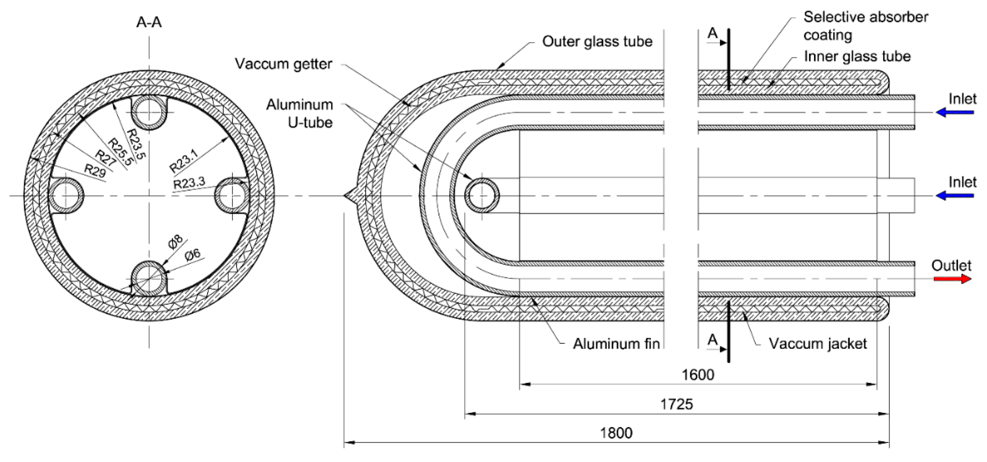
The paper puts forward an in-house mathematical model of a parabolic trough collector (PTC). The collector is fitted with a sun-tracking system with two rotation axes to increase the energy gain. The solar collector comprises evacuated tubes with a triple-wall design of the absorber and two U-tubes inside. It should be highlighted that commonly used PTC collectors are equipped with a single U-tube. Thus, the case considered seems to be an innovative construction.

Solar technologies are becoming increasingly popular these days. Sunlight as a source of energy is used to generate direct current electricity in photovoltaic (PV) panels and to produce heat in solar collectors. There are also hybrid photovoltaic panels with flat solar collectors coupled with the PV panel to increase solar energy harvesting. Two basic types of solar collectors may be distinguished as non-concentrating and concentrating collectors. Among concentrated collectors, compound parabolic collectors (CPC) and parabolic trough collectors (PTC) draw the attention of researchers and industrial developers. The greatest assets of the concentrated collectors constitute its unique features of capturing the solar rays, including diffuse rays, no tracking mechanism at low to moderate concentrations, minimal heat loss, and higher collector efficiency. A vast review of concentrated collectors in terms of their development, experimental and theoretical study, and recent applications was presented by Pranesh et al. [1].

PTC belongs to the group of solar collectors, of which development began with their first practical application in 1898 [2]. So far, the most significant use of this type of technology is the Solar Electric Generating System (SEGS) power plant (345 MWe) [3] and Plataforma Solar de Almeria in Spain, equipped with PTCs of total capacity equal to 1.2 MW. PTC collectors can effectively generate heat between 50 °C and 400 °C [1]. Additionally, there is reliable information showing that PTC technology is adequate for generating electricity using medium temperature (~400 °C) of HTF (heat transfer fluid) [4].

The work presented in this publication refers to PTC for low-temperature residential applications. PTC has numerous applications, and research work was conducted in this area. Thus, Sayed and Sivaraman presented research on a hot water generation system using a PTC collector [5]. The twisted tape inserts were used to enhance the thermal performance of the collector. Jamadi et al. [6] compared flat-plate solar collectors (FPC) and PTC systems to heat a building space. Authors showed experimentally that the PTC system with lower occupied space could produce higher thermal energy quality compared to the FPC heating system. Zou et al. performed experimental work concerning small-sized PTC for water heating in cold areas [7]. The authors concluded that the investigated PTC could collect solar radiation efficiently, demonstrating an event with an efficiency of 67% under solar radiation of less than 310 W/m². A solid review of prototypes of PTCs used for low-temperature demands was presented in Reference [8].

PTC is commonly used in practice. Thus, it is given constant and extensive attention in the literature. Many studies were devoted to PTC efficiency improvement [9], both experimentally and numerically [10]. The literature also offers a vast number of results for experimental and theoretical computational testing carried out in the range of optical [11] and thermal parameters of the collectors [12]. The effect of the research is that PTCs are now a common and advanced structure intended for solar energy utilization. Most of the studies described in the literature related to the modeling and simulation of solar collectors were based on models making use of computational fluid dynamics (CFD) techniques. This is due to the full availability of CFD software and the relatively simple geometry of the collectors (constant along their length). Two major groups of studies on CFD models of solar collectors can be distinguished. The first comprises analyses conducted with a view to minimize heat losses to the environment. The second aims to enhance the solar collector performance via changes in design or solar fluid modifications [13], using nanofluids, for instance.

As an example of the studies from the first group, one may highlight Reference [14], which presented an analysis of compound parabolic concentrator (CPC) solar collectors mounted on a tracker with a single rotation axis. The CPC collectors, tested by the authors, used a novel solution, implementing new absorber tubes and multi-parabolic receivers with a total aperture surface area of 15.4 m². One of the tested collectors was lined with ethylene tetrafluoroethylene (ETFE) foil. The absorber tube was covered with a foil to minimize heat losses to the environment. The aim of the research was to establish the impact of the tested foil on the collector heat loss and efficiency. The authors not only carried out an experimental investigation but also built a CFD model of the new-design solar collector. The presented model reflected the full three-dimensional (3D) geometry of one row of the collector. The authors used the surface radiation model. The relative error obtained between the calculated and measured values of the fluid temperature was minimal. Even though the authors referred to their computational model as a simplified one, it contained 1.8 million computational cells mapping the collector geometry in great detail. The developed model confirmed the justification for the use of the proposed foil. However, due to the specificity of CFD calculations, the model is more suitable for steady-state testing (as performed by the authors) rather than for analyzing the collector operation in transient states.

In Reference [15], Kaloudis et al. presented the results of their research on a PTC. The work was computational in nature. Nanofluids were used as the solar fluid to investigate the impact of the content of nanoparticles on the PTC efficiency. An extended model of the collector was proposed, comprising an outer glass tube, the space in between the tubes, the tube with an absorber, and the solar fluid. The model took account of the conjugate heat transfer, and radiation was modeled using the surface-to-surface model. Heat losses to the surroundings were taken into account by setting the convective boundary condition, where the heat transfer coefficient was a function of the wind speed (a similar approach was used in many other studies, e.g., References [14,16]). The model proposed in Reference [15] was validated through a comparison with the experimental testing results available from Reference [17] (the results are widely quoted in issues related to research on PTCs). The authors’ numerical model showed that a solar fluid containing up to 4% of aluminum (III) oxide nanoparticles improved the collector efficiency by about 10%.

A computational analysis using nanofluids in a direct absorption solar collector (DASC) intended for household/non-industrial applications was conducted in References [18,19]. In Reference [19], the authors took account of the phenomenon of an increase in the absorptivity of the heat transfer fluid (HTF) depending on the amount of suspension containing carbon nanohorn particles. The variation in collector efficiency was obtained as a function of the nanoparticle concentration for two design variants of the collector (double-tube and triple-tube options). Like in other studies, the outer diameter of the solar tube or of the system built of a mirror and a solar tube was small compared to the total length of the collector under analysis. Due to the use of nanoparticles and the conjugate thermal and flow analysis solution to account for the energy source terms with due accuracy, testing of flows through the annular cross-section required a higher density of the numerical mesh in the solar fluid domain [18,19]. The considerable length of the analyzed collectors and the need to increase the numerical mesh density in the fluid domain resulted in a high number of computational elements, which makes the model less useful when it comes to transient-state analyses.

Evacuated tube solar collectors (ETSC) in a system with a water tank were analyzed in Reference [20]. The authors performed a CFD optimization study of various system parameters and their impact on the system’s thermal performance. Among the other parameters, nanoparticle ratios in water were studied. Results proved that nanoparticle copper and an increase in their volume ratio gave the highest thermal performance among the nanoparticles used in the study. Farhana et al. [21] presented a ground review of works showing the influence of nanofluid use on the thermal yield of direct absorbing solar collectors, where the latest results of experimental and computational works with CFD tools were presented.

Missirlis et al. [22] analyzed the influence of different configurations of solar collectors on heat transfer through the DASC polymeric solar collector. The author took into account a few cases, allowing redesign of the collector without increasing production costs. The application of CFD methods enabled choosing one of the possible solutions for improving the heat transfer properties of the polymeric DASC.

Reference [23] presented the results of CFD modeling of a PTC, in which annular receivers were partially filled with air. According to the authors, the solution is dedicated to PTC low-temperature applications. Non-vacuum PTCs are much cheaper than vacuum ones, but they are also affected by greater heat losses to the surroundings. Using numerical tools, Chandra et al. analyzed intermediate solutions, where the upper part of the annular space was filled with insulation, and the lower part on the side of the incident reflected concentrated radiation was filled with air. They validated their model against the testing data presented in Reference [17]. According to the authors of Reference [23], the most important conclusion drawn from their research was the reduction in convective losses by about 12.5% compared to the standard structure filled with air.

Apart from 3D models that take into account geometrical details and complex flows, one-dimensional (1D) models are also popular in the literature. These models were created a few decades ago and were developed ever since. Some of them evolved into commercial software intended for collector operation analysis, also in transient-state conditions. Among others, Hongbo et al. [24] performed calculations using four 1D models available from the literature based on the energy and mass conservation equations. The models concerned tube-in-tube PTCs. The calculations results were compared to each other and experimental data. Nevertheless, the study was related to the steady-state problem only. The authors concluded that the tested 1D model is an excellent trade-off between the simplicity of the models and their accuracy. The difference between the calculated and measured values of the fluid temperature obtained in Reference [24] was below 1 °C.

Yılmaz and Soylemez [25] presented a mathematical model of a single-pass collector mounted on a tracker with a single-rotation axis. The model contained a module for thermal and optical calculations. After the model validation (against experimental data available from the literature), the model was used to analyze the collector performance characteristics under different operating conditions. The model enabled analyzing the impact of many factors (e.g., the wind speed and optical parameters) on the collector efficiency. However, the model is intended for steady-state analyses only.

Liang et al. [26] presented a 1D mathematical model of a filled-type evacuated tube solar collector with a U-tube. The filled-type evacuated tube consisted of a glass evacuated tube, a U-tube, and a heat transfer component. To describe physical phenomena, the model proposed made use of thermal resistance equations instead of the energy equation. The model concerned steady states and was used to find the optimal value of thermal conductivity for the filling material, which ensured the highest efficiency of the collector.

A model of a classical collector with a concentrating (converging) mirror with a tube absorber in a glass envelope, enabling a transient-state analysis, was presented by Lamrani et al. [27]. The collector was fitted with a sun-tracking system. The model input data wwre meteorological graphs. Like in most other studies, the model was validated against experimental data [17]. Using the results, the authors analyzed the collector performance for a location in Morocco. They obtained conclusions concerning, among others, the maximum collector efficiency and the minimum and maximum amount of the useful heat gain per day.

Another 1D model intended for PTC transient-state performance analysis was presented by Xu et al. [28]. Like in the papers referred to above, the PTC described had an evacuated-type receiver that consisted of an absorber, a glass envelope, and a vacuum annulus. It operated in an industrial plant. The model was validated using data from a 1-MW solar plant. The authors of the study proposed a fast and straightforward model to simulate the transient-state performance of PTCs. It was observed that the model could be helpful in identifying a safe operation mode of the PTC to achieve higher useful power outputs.

The presented literature review indicates that no analysis was made so far of the operation of a sun-tracked PTC in which each repetitive segment has two U-tubes containing the solar fluid. This paper proposes a 1D distributed parameter PTC model, including the solar fluid two-pass flow through a double U-tube. The model takes account of the collector operation in unsteady-state conditions. One arm of the U-tube is in the direct radiation area and the other is in the area of reflected radiation (concentrated on the absorber). The U-tubes are installed collision-free inside a solar glass tube, the inner surface of which is in direct contact with the absorber. The collector tube has the shape of a Dewar vessel, where space in between the tubes is filled with vacuum, to reduce heat losses from the absorber. The collector design is presented together with a mathematical model and a discretized CFD model constructed according to best practice resulting from the authors’ experience and the literature review. The CFD model results are used for preliminary computational verification of the developed in-house mathematical model. The verification consists of a comparison of the values of the solar fluid temperature at the U-tube outlet obtained for different boundary conditions. The in-house model is less demanding computationally, and less time is needed to perform the calculations compared to the CFD model. The model is suitable for both steady-state analyses and simulations of the collector unsteady-state performance (real solar collectors always operate in transient conditions). The developed mathematical model is similar to the model of the flat-plate solar collector (FPC) presented in Reference [29].

The next stage of the mathematical model validation, presented herein, is its extensive experimental validation, which is planned to be performed further. A test stand is now being built for this purpose. It comprises a three-segment PTC equipped with a sun-tracking system with two axes of rotation and a data acquisition system. For the purpose of this work, the installation was put into operation for one day, and preliminary measurements, as well as comparisons, were performed.

2. Description of the Solar Collector

The primary element of the analyzed solar collector structure is an evacuated tube made of borosilicate glass. The solar collector tube has the structure of a Dewar vessel [26]; it is made of two concentric glass cylinders separated by a 1.5-mm-thick layer of vacuum. The collector tube outer and inner diameters are 58 and 47 mm, respectively. The collector tube is 1800 mm long. The vacuum-side inner wall is covered with a selective coating. The design parameters of the evacuated tube and the absorber are listed in

Table 1. Parameters of the solar collector evacuated tubes.

Glass Tube Material	Borosilicate Glass
Glass tube dimensions	length 1800 ± 10 mm
	outer diameter 58 mm
	inner diameter 47 mm
	wall thickness 1.6 mm
Vacuum	≤ 5 × 10−3 Pa
Transmissivity	0.92
Absorptive layer material	AIN/ALN-SS/Cu
Absorptivity	0.92–0.96 (AM1.5)
Emissivity	0.04–0.06

.

Inside the evacuated tube, there are two U-tubes with an outer diameter of 8 mm. The tubes are made of the 6061-T6 aluminum alloy and are rotated by 90° to each other. The contact between the U-tubes and the glass wall is ensured by a thin, springy plate made of the same material as the U-tubes, which provides appropriate pressure, the fixed position of the tubes, and better heat exchange. The space between the glass wall and the springy plate is filled with thermal paste to reduce contact resistance. The inside of the solar collector tube is filled with air. The cross-section of the solar collector tube with the U-tubes is presented in Figure 1.

To increase solar energy utilization, the evacuated-tube PTC is equipped with parabolic reflectors concentrating solar radiation. The reflectors are made of highly polished aluminum to achieve the mirror effect. The reflectors are manufactured by a multi-stage bending of the aluminum alloy sheet. The outcome is a parabolic reflector made of seven stages, where each of the stages is an appropriately bent straight segment of a polished aluminum sheet. Each reflector is 186 mm wide and 1.6 m long. According to the producer, the mirror reflectivity reaches 0.85.

Figure 2 presents the structure of the solar collector single segment made of an evacuated tube and a solar radiation concentrator built of two reflectors.

The solar concentrator reflectors are positioned to focus solar radiation on the lower half of the absorber circumference. A 46-mm gap exists in between the mirrors. The gap reduces the collector resistance to the wind, which improves the safety of the collector operation. Since the collector moves on sun-tracked systems with two axes of rotation, the gap does not reduce the aperture area (the active surface area), reflecting sunbeams toward the absorber. In fact, the gap includes the reflector area that is continuously shaded by the collector tube; within this area, the absorber captures the direct solar radiation incident on the upper part of its circumference (Figure 2).

The described design of the PTC allows varying the number of segments between three and eight in one collector, depending on the user’s heat demand. In the hydraulic system, the collector evacuated tubes are connected in parallel, which ensures a uniform flow of the solar fluid in each of them. The solar fluid, in this case, is a mixture of propylene glycol and water with a mass concentration of 50%.

The solar collector analyzed herein is made of three segments (Figure 3). This particular collector, being a part of the test stand (currently under construction), will be used in the future for experimental verification of the results obtained from the collector in-house mathematical model described in Section 3 below.

3. Model Development

This section presents a proposal for a mathematical model of the PTC described in Section 2. It is a one-dimensional (1D) distributed parameter model that is used to simulate the solar collector unsteady-state operation under any variable boundary conditions. Five nodes are taken into consideration in each cross-section of every segment, both in the direct and in the concentrated radiation area (Figure 4). The nodes cover the inner and the outer solar tube, two layers of the absorber (in the form of thin aluminum sheets), and the solar fluid flowing through the U-tubes. The inner solar tube is divided into two control volumes. For the air inside the collector, the impact of direct and concentrated radiation is taken into account. It is assumed that the U-tubes are a part of absorber 2. Thus, in each analyzed cross-section of the collector, 11 nodes are obtained, for which energy balance equations are formulated. In this way, an 11 × N-node model is obtained, where N denotes the number of nodes (the number of control volumes) in the direction of the fluid flow inside the U-tubes.

A basic simplification of the developed model is that the heat conduction in the circumferential direction by the aluminum lamellae, constituting the collector absorber, is omitted. The simplification is adopted to substantially reduce the number of differential equations solved at the same time, which makes it possible to obtain results much faster. The effect of this approach is uniform “heating” of absorbers to different temperatures in the area of direct and concentrated radiation. However, these temperatures will have a constant value on the respective circumference parts (falling on a given radiation area). Considering the high thermal conductivity of aluminum, in real conditions, the absorber in the direct radiation area will heat up quickly due to the heat conduction from the area of concentrated radiation. This will cause a temperature t_a1 and t_a2 increase in the circumference of absorbers (Figure 4). In the proposed model, each of the absorber N control volumes has a constant temperature on the part of the circumference exposed to the direct and concentrated radiation. As a result, the absorbers and the fluid temperature distributions along the U-tube length, obtained from the developed model, will be different compared to real conditions. The approach described in Section 5 is proposed in the developed model in order to partially take into account the heat conduction in the circumferential direction.

Nonetheless, the total heat flux absorbed by the fluid will be the same in both cases. Therefore, the solar fluid temperature obtained from the proposed model at the collector outlet will be the same as in real conditions. The 3D model of the solar collector was also developed (Section 4) to confirm this assumption. The 3D model takes entirely into account the heat conduction in the circumferential, radial, and axial direction (in all computational domains). Selected results are compared in Section 5.

In the case of non-uniform heating on the circumference of thick-walled tubes made of a material with a much lower thermal conductivity coefficient (e.g., steel tubes), high thermal stresses may arise and affect operational safety. The stresses are the effect of significant temperature differences on the tube circumference and the tube wall thickness. It is then necessary for the mathematical model to take account of heat conduction in the circumferential and radial direction [30,31]. However, this lengthens the computation time considerably with no effect on the accuracy of determination of the fluid temperature at the tube outlet.

The other assumptions adopted in the collector mathematical model are as follows:

-

Each segment of the collector operates in the same thermal and flow conditions;

-

The fluid flow is uniform in all U-tubes of the collector composed of any number of segments;

-

The heating of the walls of the U-tubes (being a part of absorber 2) is uniform on the circumference;

-

The solar radiation reflected from the reflector (and concentrated on the absorber) is related to the outer surface of absorber 1 with diameter d_ab (Figure 4);

-

The fluid and the absorber material physical properties are calculated on-line as a function of temperature;

-

Physical properties of solar tubes are assumed as constant;

-

On-line calculations are carried out of the coefficient of the heat transfer from the U-tube inner surface to the fluid;

-

The collector loses heat to the environment via convection and radiation (conditions set on the outer surface of the outer glass tube);

-

The radiative heat transfer occurs between the inner and the outer solar tube (due to vacuum, there is no convection);

-

The air inside the collector is heated due to convection from absorber 2 (the air temperature is the effect of both direct and concentrated radiation);

-

The radiative heat transfer occurs between the inner surfaces of absorber 2 (between the areas with temperatures t_a4 and t_a2, in the area of concentrated and direct radiation, respectively).

The assumptions formulated above do not simplify the model and do not change the physics phenomena occurring in the solar collector. They rather indicate the model complexity, e.g., taking into account radiative heat transfer between the inner surfaces of the absorber 2, as well as the on-line calculation of physical properties of the heat transfer fluid and absorbers. It should be noted that it is assumed that the temperature-independent physical properties of solar tubes do not affect the calculation results. The physical properties of the solar tubes change slightly, and the thermal conductivity remains constant and reaches 1.0 W/(m·K) within the working temperature range. Considering the small number of segments installed (Figure 3), inequalities of the medium flow distribution through the separate U-tubes are negligible. Moreover, such a high thermal conductivity value of aluminum causes the U-tube to heat up quickly and equalize its temperature around the perimeter. Therefore, a one-dimensional heat transfer model is adopted in this case.

When considering the symmetry of the system, the energy balance equations for all elements of the collector (all the collector nodes) are written below in relation to one U-tube of one segment. The equations are derived for the area of direct radiation and the area of radiation reflected from the reflector (concentrated on the receiver).

The energy balance equations are written first for the control volume of one U-tube (Figure 4) in the direct radiation area.

– Outer solar tube:

$$C_{g1}\frac{\mathrm{d}{t}_{g1}}{\mathrm{d}\tau }={\Phi }_{am}+{\Phi }_{r1}+{\Phi }_{s1},$$

(1)

where C_g1—thermal capacity of the outer glass tube, J/K; t_g1—temperature of the outer glass tube, °C; τ—time, s; Φ_am—heat flux lost to the environment, W; Φ_r1—heat flux exchanged between solar tubes due to radiation, W; Φ_s1—solar heat flux absorbed by the outer glass tube, W.

– Inner solar tube (control volume with node t_g2):

$$C_{g2}\frac{\mathrm{d}{t}_{g2}}{\mathrm{d}\tau }={\Phi }_{c1}+{\Phi }_{r1}+{\Phi }_{s2},$$

(2)

where C_g2—thermal capacity of the analyzed control volume of the inner glass tube, J/K; t_g2—temperature of the inner glass tube, °C; Φ_c1—heat flux conducted in the radial direction by the inner glass tube, W; Φ_s2—solar heat flux absorbed by the analyzed control volume of the inner glass tube, W.

– Inner solar tube/absorber 1 (control volume with node t_a1):

$$C_{a1}\frac{\mathrm{d}{t}_{a1}}{\mathrm{d}\tau }={\Phi }_{c1}+{\Phi }_{c2}+{\Phi }_{s3},$$

(3)

where C_a1—thermal capacity of the analyzed control volume, J/K; t_a1—temperature of absorber 1, °C; Φ_c2—heat flux conducted in the radial direction by both layers of the absorber, W; Φ_s3—solar heat flux absorbed by absorber 1, W.

– Absorber 2:

$$C_{a2}\frac{\mathrm{d}{t}_{a2}}{\mathrm{d}\tau }={\Phi }_{c2}+{\Phi }_{conv}+{\Phi }_{r2}+{\Phi }_{conv,f},$$

(4)

where C_a2—thermal capacity of absorber 2, J/K; t_a2—temperature of absorber 2, °C; Φ_conv—heat flux transferred by convection to the air inside the collector, W; Φ_r2—heat flux exchanged by radiation between the surfaces of absorber 2 (in the area of concentrated and direct radiation), W; Φ _conv,f—heat flux transferred by convection to the fluid inside the U-tube, W.

– Solar fluid:

$$C_f\frac{\mathrm{d}{t}_f}{\mathrm{d}\tau }={\Phi }_{f1}-{\Phi }_{f2}+{\Phi }_{conv,f},$$

(5)

where C_f—thermal capacity of the fluid, J/K; t_f—fluid temperature, °C; Φ_f1—heat flux flowing into the control volume with the fluid, W; Φ_f2—heat flux flowing out of the control volume with the fluid, W.

The energy balance equations below relate to the control volume of one U-tube (Figure 4) in the area of radiation reflected from the reflector (concentrated on the absorber—subscript: cd).

– Outer solar tube:

$$C_{g3}\frac{\mathrm{d}{t}_{g3}}{\mathrm{d}\tau }={\Phi }_{am,cd}+{\Phi }_{r1,cd}+{\Phi }_{s1,cd},$$

(6)

where C_g3—thermal capacity of the outer glass tube, J/K; t_g3—temperature of the outer glass tube, °C; Φ_am,cd—heat flux lost to the environment, W; Φ_r1,cd—heat flux exchanged between solar tubes due to radiation, W; Φ_s1,cd—solar heat flux absorbed by the outer glass tube, W.

– Inner solar tube (control volume with node t_g4):

$$C_{g4}\frac{\mathrm{d}{t}_{g4}}{\mathrm{d}\tau }={\Phi }_{c1,cd}+{\Phi }_{r1,cd}+{\Phi }_{s2,cd},$$

(7)

where C_g4—thermal capacity of the analyzed control volume of the inner glass tube, J/K; t_g4—temperature of the inner glass tube, °C; Φ_c1,cd—heat flux conducted in the radial direction by the inner glass tube, W; Φ_s2,cd—solar heat flux absorbed by the analyzed control volume of the inner glass tube, W.

– Inner solar tube/absorber 1 (control volume with node t_a3):

$$C_{a3}\frac{\mathrm{d}{t}_{a3}}{\mathrm{d}\tau }={\Phi }_{c1,cd}+{\Phi }_{c2,cd}+{\Phi }_{s3,cd},$$

(8)

where C_a3—thermal capacity of the analyzed control volume, J/K; t_a3—temperature of absorber 1, °C; Φ_c2,cd—heat flux conducted in the radial direction by both layers of the absorber, W; Φ_s3,cd—solar heat flux absorbed by absorber 1, W.

– Absorber 2:

$$C_{a4}\frac{\mathrm{d}{t}_{a4}}{\mathrm{d}\tau }={\Phi }_{c2,cd}+{\Phi }_{conv,cd}+{\Phi }_{r2}+{\Phi }_{conv,f,cd},$$

(9)

where C_a4—thermal capacity of absorber 2, J/K; t_a4—temperature of absorber 2, °C; Φ_conv,cd—heat flux transferred by convection to the air inside the collector, W; Φ_conv,f,cd—heat flux transferred by convection to the fluid inside the U-tube, W.

– Solar fluid:

$$C_{f,cd}\frac{\mathrm{d}{t}_{f,cd}}{\mathrm{d}\tau }={\Phi }_{f1,cd}-{\Phi }_{f2,cd}+{\Phi }_{conv,f,cd},$$

(10)

where C_f,cd—thermal capacity of the fluid, J/K; t_f,cd—fluid temperature, °C; Φ_f1,cd—heat flux flowing into the control volume with the fluid, W; Φ_f2,cd—heat flux flowing out of the control volume with the fluid, W.

The last energy balance equation relates to the air inside the collector. The air temperature is the effect of heat transferred from absorber 2 in the direct and concentrated radiation area. The energy balance equation has the following form:

$$C_{air}\frac{\mathrm{d}{t}_{air}}{\mathrm{d}\tau }={\Phi }_{conv}+{\Phi }_{conv,cd},$$

(11)

where C_air—thermal capacity of air, J/K; t_air—air temperature, °C.

In each analyzed cross-section of the collector, 11 differential equations are obtained. The equations are solved by approximating derivatives using appropriate difference schemes. The relations derived in the process make it possible to calculate temperature histories in 11 nodes of each control volume of the collector, and they are characterized by simple notation. Therefore, results can be obtained very quickly. The in-house computational program, written based on the derived relations, additionally makes it possible to conduct a detailed analysis of the impact of each term of the equation on the results. The method is iterative. All thermophysical properties are calculated on-line as a function of temperature using the relations given in Section 4. The heat transfer coefficient values are also calculated on-line.

In order to obtain a stable numerical solution, the time and spatial steps are selected to meet the Courant–Friedrichs–Lewy condition for one-dimensional problems as follows [32]:

$$\Delta \tau \le \frac{\Delta z}{w},$$

(12)

where Δτ—time step for the calculations, s; Δz—spatial step (length of the collector control volume), m; w—fluid flow velocity in U-tubes, m/s.

The values of concentrated solar radiation are calculated using the following balance equation (Figure 4):

$$G_d(W-d_{gl})L=G_{cd}\frac{\pi d_{ab}}{2}L,$$

(13)

which gives

$$G_{cd}=\frac{2G_d\left(W-d_{gl}\right)}{\pi d_{ab}},$$

(14)

where d_gl—diameter of the outer solar tube, m; d_ab—outer diameter of the absorber, m; G_d—intensity of direct solar radiation, W/m²; G_cd—intensity of concentrated solar radiation, W/m²; L—absorber length, m; W—reflector width, m (W = 0.418 m—Figure 2).

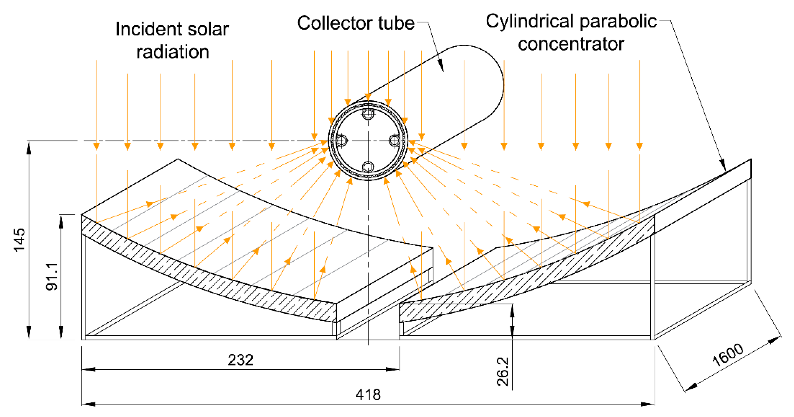
In the model developed, the influence of mutual shading of individual tubes was omitted, since the solar collector is assembled with a two-axis sun-tracking system. It becomes a significant improvement over industrial applications where one-axis sun-tracking is commonly applied. In the two-axis tracking, the collector plane is always set perpendicularly to the incident solar radiation, which avoids shading. On the other hand, in a one-axis tracking system, shading may still occur.

The derived relations are valid for the analyzed vacuum solar PTC built of any number of repetitive segments. The proposed model is also suitable (after necessary corrections to the equations) for a collector with a single solar tube (no vacuum) or with a single U-tube inside the solar tube. After some structure-related simplifications, the model is also valid for the most popular concentrating solar collectors with the absorber in the form of a single straight tube.

Firstly, in order to verify the proposed 1D model, an additional 3D model of the analyzed collector was built in the ANSYS Fluent environment (Section 4). The 3D model includes the following domains: absorbers, U-tube, heat transfer fluid, and air inside the collector. Therefore, in the 3D model, solar tubes are omitted, since the model was developed to compare, with the 1D model results, the transient temperature courses of the heat transfer. Accuracy of the 1D model depends significantly on the adopted time and spatial steps, Δτ and Δz, respectively. Thus, a comparison of the 1D and 3D model results is aimed at finding such time–space step values, for which a satisfactory correspondence of the calculation results is obtained.

In addition to the computational verification, a pre-experimental verification using the Δτ and Δz steps identified was also performed. The test stand, currently still under construction, was started for one day, to enable the necessary measurements to be made.

Extensive experimental verification of the 1D model is planned to be carried out in the future, using the Δτ and Δz values verified in this article.

4. 3D CFD Model

This section presents the simulation model and methodology used to simulate the operation of the U-tube parabolic trough collector (PTC). The collector model was built using the ANSYS Fluent 19.3 code [33], where thermal and fluid dynamic analyses can be performed simultaneously. This software is the leading tool for flow and heat simulations. It was also used in previous studies to simulate various solar thermal collectors [12,18,23,34]. The developed model is three-dimensional. It is assumed that the model is symmetrical, and the symmetry plane is the YZ surface passing through the center of the solar pipe. Water flows through the upper tube of the absorber, then turns on the U-tube and flows in the second pass through the lower tube, as shown in Figure 1 and Figure 4. A modification is introduced here, whereby the tube is shifted to keep the symmetry plane. In the real object, the first and the second pass are in different halves of the solar pipe, as described in Section 2 (see Figure 1). In the collector model geometry, the second and the first pass are in the same half. This approach is correct because the upper pipe is in the direct radiation area, and the lower pipe is in the concentrated radiation area. This simplification makes it possible to achieve a more economical model without compromising the model reliability.

The model omits the glass tubes and the vacuum space between them. The thermal load on the absorber surface in the direct and in the concentrated radiation area is reduced by losses to the environment and losses due to thermal resistance of the glass tubes and vacuum. The direct and concentrated radiation areas are marked in Figure 5 as Wall_d and Wall_c, respectively. The geometric model is 1600.0 mm long, and the diameter of the outer domain corresponding to the outer diameter of the tube formed by the sheet metal of absorber 1 is 47 mm (Figure 1). The other dimensions of the U-tube and metal sheets are as shown in Section 2 in Figure 1. The model takes into account that the space between the U-tube and the metal sheets is filled with thermal paste.

The governing equations of the computational fluid dynamics (CFD) analysis include the mass conservation equation, the momentum conservation equation, and the energy conservation equation. The CFD model calculates the conjugate heat transfer between the fluid and the solid material, the convective heat transfer in the fluid regions, and heat radiation. Radiation q_rad in the model occurs on the inner surface of the inner metal sheet due to temperature non-uniformity (Figure 5). The non-uniformity is the effect of the heat flux values affecting the upper and the lower half of the outer metal sheet and of the HTF interaction. The radiative heat transfer inside the collector was calculated using the surface-to-surface (S2S) radiation model.

The HTF physical properties are assumed to be temperature-dependent. The following equations for density, specific heat, thermal conductivity, and viscosity calculations with respect to temperature were introduced into the CFD model:

ρ = 1264.278 − 0.76449∙T,

(15)

c_p = 2490.163 + 3.474011∙T,

(16)

k = 0.301316 + 0.000304∙T,

(17)

μ = − 7.07771 × 10⁻⁹∙T ³ + 8.26006∙10⁻⁶∙T ² − 3.20788 × 10⁻³∙T + 4.15210 × 10⁻¹,

(18)

where T is the fluid temperature in K.

The above equations are valid in the temperature range from 0 °C to 100 °C and are the same as those used in the in-house program. Similarly, the properties of aluminum (specific heat and thermal conductivity) were introduced into the model according to the following equations [35]:

c_p = 917.2217869 + 0.7560459783∙t − 0.00135558959∙t ² + 1.794154854 × 10⁻⁶∙t ³,

(19)

k = 162.4121535 + 0.1517238301∙t − 2.574634293 × 10⁻⁵∙t ²,

(20)

where t is the solid temperature in °C.

The velocity of the HTF flowing through the collector tubes is low, from about a few mm/s to about a dozen cm/s [36]. The Reynolds number values range only from a dozen to several hundred when considering such a small diameter of the tubes. Thus, the Reynolds number value is much lower than the critical value of Re_cr = 2300 [29,36]. Due to the above, it is assumed that the HTF flow is laminar.

The boundary conditions assigned to the CFD model are as follows:

▪

Inlet—a uniform velocity inlet boundary condition is adopted at the U-tube inlet where v_z = v, v_y = v_y = 0; T = T_in;

▪

Outlet—an outflow boundary condition is used at the U-tube outlet;

▪

Wall—no-slip conditions on the inner absorber surfaces;

▪

The top outer wall (Wall_d) of the absorber is subjected to heat flux Gd, which corresponds to the heat load from the direct radiation area;

▪

The bottom outer wall (Wall_c) of the absorber is subjected to heat flux Gcd, which corresponds to the heat load from the concentrated radiation area.

The calculations start with the initial condition of zero velocity and uniform temperature throughout the calculation domains. The calculations are performed using the coupled algorithm and PRESTO! discretization for pressure, while the second-order upwind approach is followed for other quantities. The numerical solutions are convergent when the residuals of continuity and of the momentum equations are less than 10⁻⁴, and the residuals of the energy equation are less than 10⁻⁷. Furthermore, the convergence criterion must ensure that the mass-weighted average temperature at the outlet is constant.

A hexahedral-dominant mesh is created to discretize the computational domain to obtain results with high levels of accuracy. There is a substantial difference between the dimension of the tube length (1600 mm) and the absorber tube outer diameter (47 mm). Moreover, the HTF flow in the U-tube has a significant impact on collector thermal efficiency. Due to that, a fine mesh is required in the cross-section of the computational domain with a refined mesh along the U-tube perimeter. The refined boundary-layer mesh is also applied to the inner surface of absorber 2 on the air-washed sides (to capture the air movement caused by natural convection as a result of air heating and the difference in density). Figure 6 illustrates the front cross-section divided into control volumes. The model has 1.1 × 10⁶ elements. It is built by sharing the frontal surface of the model (Figure 6) in the first place. The grid was compacted in the areas of expected large gradients in the wall-fluid contact areas. Mesh tools are adopted to create the hexa dominant mesh. Then, the mesh is created on the frontal surface, and the periodic mesh operation is used to generate the entire mesh of the PTC collector model. This way, the dominant hexa mesh is obtained, and the division of the model into subdomains connected by interfaces is avoided.

The CFD model is a model where coupled heat transfer is considered, and the results are affected by the division of the domain into control volumes. Therefore, the grid independence study was performed to make sure that the numerical solution is independent of the mesh resolution. The parameters for the grid-independent verification test include the overall heat transfer rate from the absorber tube wall to heat transfer fluid, and the HTF outlet temperature. The grid independence study was carried out for four grids with the following element numbers: 0.5 × 10⁶, 0.71 × 10⁶, 1.1 × 10⁶, and 1.7 × 10⁶. As a result, the outlet temperature of the HTF remained constant when the number of elements was greater than 1.0 × 10⁶. Therefore, the model with the number of elements equal to 1.1 × 10⁶ was selected for CFD analysis based on the comprehensive consideration of computational time and accuracy of the results obtained.

5. Results and Discussion

Firstly, a number of calculations were performed for different boundary conditions to verify the accuracy of the results obtained from the in-house mathematical model of the collector. The same conditions were also used to carry out CFD calculations. Selected results of the calculations and comparisons are presented in

Table 2. Comparison of the fluid temperature at the solar collector outlet obtained from the proposed mathematical model and from the CFD calculations for different assumed solar radiation intensity values and different volume fluxes of the fluid.

Solar radiation intensity, W/m2		600			800			1000
Total volume flux of the fluid flowing through the collector, L/min		1	1.5	2	1	1.5	2	1	1.5	2
Fluid velocity in one U-tube, m/s		0.0982	0.1474	0.1965	0.0982	0.1474	0.1965	0.0982	0.1474	0.1965
Fluid temperature, °C	Mathematical model (tm)	48.68	45.51	44.40	51.55	47.76	45.90	54.99	49.99	47.60
	CFD (tCFD)	48.76	45.59	44.36	51.47	47.83	45.94	55.09	49.93	47.50
Δt = ǀ tm – tCFD ǀ, °C		0.08	0.08	0.04	0.08	0.07	0.04	0.10	0.06	0.10
ǀ tm – tCFD ǀ / tCFD, %		0.16	0.17	0.09	0.16	0.15	0.09	0.18	0.12	0.21

and in Figure 7, Figure 8, Figure 9 and Figure 10.

The 3D CFD model (Section 4) takes no account of the two solar tubes, which is due to the fact that the model was developed to verify the in-house model comprising only the most essential elements of the solar collector, i.e., absorbers, U-tubes, and the solar fluid. It was not the task of the 3D model to precisely map the entirety of the occurring phenomena, which was the case in other works, e.g., References [23,34]. For this reason, the heat flux set on the absorber outer walls (Wall_d and Wall_c) was the same as in the in-house model, as were the mass flux and the HTF temperature. The calculations aim to verify the correctness of the fluid temperature at the collector outlet determined using the in-house model (the 1D model should satisfy the mass and energy balance). Considering the above, the aspects of solar radiation transmissivity through the glass division walls are omitted in the developed 3D model.

The assumed volume fluxes of the fluid shown in Table 2 relate to the entire collector, built of three segments (Figure 3). Considering that, in every segment, there are two U-tubes, it is assumed that the fluid flows uniformly through six U-tubes (Table 2 shows the assumed flow velocity in one U-tube). The calculations were performed for three selected heat flux values of solar radiation. i.e., 600, 800, and 1000 W/m². In each analyzed case, it is assumed that the initial temperature distributions in the two absorbers, in the fluid and in the air inside the collector, are the same and total 40 °C. Moreover, in the developed in-house model, it is assumed that the initial temperature distribution of the outer solar tube is equal to the ambient temperature of 20 °C. The initial temperature distribution of the inner solar tube is assumed as uniform and equal to 40 °C. The assumed wind speed totals 3 m/s.

Satisfactory agreement between the developed 1D model and the 3D CFD model results was obtained for calculations performed using the in-house model with the time step of 0.001 s and the spatial step of 0.04 m. In total, 80 control volumes were obtained in the direct and concentrated radiation area. Considering that there are 11 nodes in every control volume (Figure 4), 880 differential equations were solved in every time instant. The computational program is written in the Fortran code [37].

When analyzing Table 2, it can be seen that the fluid temperature at the collector outlet obtained from the in-house model differs from the CFD model value by 0.1 °C maximum, which means that the error totals about 0.21%. The obtained agreement between the results should be considered as fully satisfactory. The time of the in-house model calculations (until the steady state was achieved) totaled about one minute. Such a short computation time, at the fully satisfactory accuracy of the result, is a fundamental advantage of the developed in-house model.

The equivalent value of the heat flux absorbed partially by the absorbers in the direct radiation area (Figure 4) is determined to take into account partial heat conduction of both absorbers in the circumferential direction. In real conditions, these parts of the absorbers will heat up quickly due to heat conduction in the circumferential direction. The heating is simulated using the equivalent heat flux value found from the balance Equation (21). In the equation, it is taken into account that, in real conditions in the direct radiation area, solar radiation is absorbed by the surface $\frac{d_{ab}\cdot \Delta z}{2}$, whereas, in the concentrated radiation area, it is absorbed by the surface $\frac{\pi \cdot d_{ab}\cdot \Delta z}{4}$. Assuming that the heat flux with equivalent intensity G_equiv is absorbed in the concentrated radiation area, and that half of this value is absorbed in the direct radiation area, the following balance equation can be written:

$$G_d\frac{d_{ab}}{2}+G_{cd}\frac{\pi d_{ab}}{4}=\frac{1}{2}{G}_{equiv}\frac{\pi d_{ab}}{4}+G_{equiv}\frac{\pi d_{ab}}{4}.$$

(21)

After relevant transformations, the following relation is obtained (the relation was used to calculate the equivalent value of the solar radiation intensity):

$$G_{equiv}=\frac{4G_d+2\pi G_{cd}}{3\pi }.$$

(22)

Selected results of calculations and comparisons for the assumed solar radiation intensity G = 600 W/m² are shown in Figure 7 and Figure 8, and those for G = 1000 W/m² are shown in Figure 9 and Figure 10. In both cases, the volume flux of the fluid flowing through the entire solar collector (built of three segments) totals 1 L/min. The computational mass flux of the fluid flowing through one U-tube is 0.00285 kg/s.

Figure 7 and Figure 9 present a comparison of the fluid temperature distribution along its flow path through the U-tube for the final steady state. The U-tube total length in contact with the absorber is 3.2 m (1.6 m in the direct and in the concentrated radiation area, respectively). As expected, the distributions obtained from the developed in-house model differ from those produced by the 3D CFD model.

Since the heat conduction is omitted in the 1D model, the fluid in the direct radiation area gains temperature more slowly than when considering the heat conduction (3D model). Consequently, the high temperature of the absorbers in the concentrated radiation area causes a rapid increase in the fluid temperature for the 1D model.

The situation is entirely different for the 3D model, where heat conduction in the circumferential, axial, and longitudinal directions is fully considered. In this case, the working fluid heats up faster in the direct radiation area (compared to model 1D) because the absorbers reach a higher temperature in this section (due to heat conduction from the concentrated radiation area). At the same time, the heat drain in the absorbers from the concentrated radiation area causes the fluid to heat slowly in this area. Thus, the temperature distributions of the fluid, obtained by means of the 3D model (Figure 7 and Figure 9), are characterized by a smooth course. The distributions obtained using the 1D model indicate specific refraction of these distributions over the U-tube length of 1.6 m, i.e., where the direct radiation ends and the concentrated radiation starts to act. The analysis of Figure 7 and Figure 9 shows that, in spite of different distributions along the U-tube length, the temperature of the fluid at the outlet, obtained by means of both models, is the same (at 3.2 m—outlet cross-section).

To confirm the adopted assumption that, regardless of different temperature distributions on the circumference of absorbers, the total heat flux absorbed by the fluid will be the same in both models (especially when absorbers are made of a high thermal conductivity material), Figure 8 and Figure 10 present comparisons of the fluid temperature histories at the U-tube outlet. A slightly bigger difference can be noticed in Figure 8 for the time interval of about 200 s to about 300 s. The maximum difference is about 0.25 °C, which is negligibly small. It may, therefore, be stated that the agreement observed in Figure 8 and Figure 10 between the histories of the fluid temperature at the collector outlet obtained from the in-house 1D model and the 3D CFD model is fully satisfactory. This confirms the correctness of the adopted assumption that the total heat flux absorbed by the fluid does not depend on the temperature distribution on the absorber circumference (omitting heat conduction in the circumferential direction of absorbers in the in-house model does not generate errors in the results of the calculations of the fluid temperature at the U-tube outlet). It also confirms the effectiveness of the developed mathematical model and its usefulness for simulations of the operation of vacuum solar parabolic trough collectors. In calculations of thermal systems equipped with solar collectors, the user’s/designer’s attention is focused on the achieved value of the fluid temperature at the collector outlet and not on the temperature distribution on the collector length.

As mentioned earlier, in both cases (1D and 3D models), the total heat flux absorbed by the fluid along the entire length of the U-tube is the same. Therefore, the temperature of the fluid at the collector outlet (only at the outlet) is the same. To further confirm this phenomenon, the computed values of the heat flux absorbed by the fluid along the length of the U-tube in both models are given below in

Table 3. Heat flow rate absorbed by the fluid (one-dimensional (1D) model).

Direst Radiation Area				Concentrated Radiation Area
U-tube longitudinal coordinate, m	${\dot{Q}}_d$, W	U-tube longitudinal coordinate, m	${\dot{Q}}_d$, W	U-tube longitudinal coordinate, m	${\dot{Q}}_{cd}$, W	U-tube longitudinal coordinate, m	${\dot{Q}}_{cd}$, W
0.04	0.9332	0.84	0.9087	1.64	1.3525	2.44	1.3125
0.08	0.9337	0.88	0.9088	1.68	1.3507	2.48	1.3127
0.12	0.9343	0.92	0.9093	1.72	1.3510	2.52	1.3129
0.16	0.9340	0.96	0.9097	1.76	1.3512	2.56	1.3109
0.20	0.9307	1.00	0.9102	1.80	1.3492	2.60	1.3111
0.24	0.9296	1.04	0.9075	1.84	1.3494	2.64	1.3101
0.28	0.9239	1.08	0.9065	1.88	1.3496	2.68	1.3093
0.32	0.9151	1.12	0.8957	1.92	1.3476	2.72	1.3095
0.36	0.9103	1.16	0.8929	1.96	1.3472	2.76	1.3078
0.40	0.9103	1.20	0.8935	2.00	1.3376	2.80	1.3084
0.44	0.9104	1.24	0.8920	2.04	1.3269	2.84	1.3090
0.48	0.9105	1.28	0.8923	2.08	1.3178	2.88	1.3068
0.52	0.9088	1.32	0.8928	2.12	1.3177	2.92	1.3069
0.56	0.9093	1.36	0.8933	2.16	1.3179	2.96	1.3069
0.60	0.9097	1.40	0.8915	2.20	1.3158	3.00	1.3048
0.64	0.9102	1.44	0.8920	2.24	1.3159	3.04	1.3050
0.68	0.9086	1.48	0.8925	2.28	1.3162	3.08	1.3052
0.72	0.9090	1.52	0.8928	2.32	1.3141	3.12	1.3017
0.76	0.9095	1.56	0.8908	2.36	1.3143	3.16	1.2946
0.80	0.9100	1.60	0.8909	2.40	1.3145	3.20	1.2752
The sum ${\dot{Q}}_d$ = 36.31 W				The sum ${\dot{Q}}_{cd}$ = 52.78 W
${\dot{Q}}_t={\dot{Q}}_d+Q_{cd}$ = 89.09 W

and

Table 4. Heat flow rate absorbed by the fluid (three-dimensional (3D) CFD model).

Direst Radiation Area				Concentrated Radiation Area
U-tube longitudinal coordinate, m	${\dot{Q}}_d$, W	U-tube longitudinal coordinate, m	${\dot{Q}}_d$, W	U-tube longitudinal coordinate, m	${\dot{Q}}_{cd}$, W	U-tube longitudinal coordinate, m	${\dot{Q}}_{cd}$, W
0.04	2.254	0.84	1.406	1.64	1.266	2.44	0.839
0.08	1.918	0.88	1.395	1.68	1.211	2.48	0.822
0.12	1.825	0.92	1.382	1.72	1.199	2.52	0.805
0.16	1.771	0.96	1.363	1.76	1.165	2.56	0.795
0.20	1.723	1.00	1.344	1.80	1.136	2.60	0.778
0.24	1.687	1.04	1.325	1.84	1.111	2.64	0.762
0.28	1.658	1.08	1.308	1.88	1.083	2.68	0.743
0.32	1.628	1.12	1.291	1.92	1.055	2.72	0.730
0.36	1.609	1.16	1.278	1.96	1.055	2.76	0.712
0.40	1.590	1.20	1.258	2.00	1.015	2.80	0.686
0.44	1.566	1.24	1.241	2.04	0.991	2.84	0.680
0.48	1.547	1.28	1.218	2.08	0.945	2.88	0.646
0.52	1.531	1.32	1.190	2.12	0.922	2.92	0.591
0.56	1.516	1.36	1.168	2.16	0.926	2.96	0.543
0.60	1.503	1.40	1.137	2.20	0.944	3.00	0.527
0.64	1.489	1.44	1.110	2.24	0.932	3.04	0.460
0.68	1.474	1.48	1.077	2.28	0.918	3.08	0.398
0.72	1.454	1.52	1.012	2.32	0.903	3.12	0.306
0.76	1.440	1.56	1.007	2.36	0.883	3.16	0.220
0.80	1.419	1.60	1.005	2.40	0.853	3.20	0.211
The sum ${\dot{Q}}_d$ = 57.12 W				The sum ${\dot{Q}}_{cd}$ = 32.77 W
${\dot{Q}}_t={\dot{Q}}_d+Q_{cd}$ = 89.89 W

. These values refer to steady state. Since, in the case of the 1D model, the assumed spatial step of the calculation is z = 0.04 m, 40 cross-sections are obtained in both radiation areas. Computed values of heat fluxes were summed up and compared with the values obtained from the 3D model (Table 4). The tables refer to the data based on which Figure 7 and Figure 8 were developed (G = 600 W/m², ${\dot{V}}_t=1 \mathrm{L}/min$).

For the 1D model, in each analyzed section, the heat flux absorbed by the fluid was calculated as follows:

$$\dot{Q}=h\cdot \pi \cdot d_{in}\cdot \Delta z\cdot \left(t_a-t_f\right),$$

(23)

where h—heat transfer coefficient from the inner surface of the U-tube to the fluid, W/(m²K); d_in—internal diameter of the U-tube, m; t_a—absorber temperature, °C; t_f—fluid temperature, °C.

The temperature of the fluid at the outlet of the U-tube is, therefore, equal to

$$t_{f,o}=t_{f,in}\frac{\dot{Q}}{{\dot{m}}_f\cdot c_f}=40+\frac{89.09}{0.00285\cdot 3600}=48.68\hspace{0.17em}[℃].$$

(24)

In order to illustrate the differences in the heat fluxes absorbed by the fluid in the individual sections of both models, the 3D CFD U-tube model was also divided into 40 control volumes in both radiation areas. The calculation results are presented in Table 4.

For the 3D CFD model, the fluid temperature at the U-tube outlet is equal to

$$t_{f,o}=t_{f,in}\frac{\dot{Q}}{{\dot{m}}_f\cdot c_f}=40+\frac{89.89}{0.00285\cdot 3600}=48.76\hspace{0.17em}[℃].$$

(25)

In the equations above, it is assumed that the specific heat of 50% propylene glycol is 3600 J/(kg·K). The obtained temperature values are in accordance with the values given in Table 2 and shown in Figure 7 and Figure 8 (for the steady-state operation in the outlet section of the collector tube).

An analysis of Table 3 and Table 4 indicates that different values of the heat flux absorbed by the working fluid along the solar tube length, respectively, in 1D and 3D models, occurred. However, the total (summary) values of the heat flux absorbed along the whole U-tube length are almost the same in both cases. The temperatures of the fluid at the outlet of the U-tube are, therefore, the same. In the case of the 1D model (Table 3), in the individual cross-sections of the direct radiation area, the heat flux absorbed by the fluid changes slightly, similarly, in the area of concentrated radiation, where the heat flux is larger. This is due to the fact that the heat conduction in the absorbers from the concentrated radiation area to the direct radiation area is not included in the 1D model. The inclusion of heat conduction in the 3D model causes a visible decrease in the heat flux absorbed by fluid along both arms of the U-tube (Table 4).

In order to confirm the conclusions of the computational verification, a preliminary experimental verification was also carried out. The research stand is not yet fully completed, but it was possible to run it for one day and carry out the measurements necessary for the purpose of the article. Selected results of the measurements and comparisons are shown in Figure 11, Figure 12, Figure 13 and Figure 14. Figure 11 shows the intensity of solar radiation (heat flux of solar radiation) measured with a pyranometer. The total volume flow of the working fluid flowing through the collector (Figure 12) and the ambient temperature were also measured.

Figure 13 shows the measured inlet and outlet temperatures of the working fluid along with the outlet temperature, computed with the proposed 1D model. The measured solar radiation intensity, fluid volume flow, and its temperature at the collector inlet, as well as ambient temperature, were the input data for the computations. The analysis of Figure 13 shows that the measured and computed outlet collector temperature is fully satisfactory. To illustrate this comparison in more detail, a section of Figure 13, covering a shorter period, is shown in Figure 14.

These comparisons, being the preliminary experimental verification of the developed 1D model, fully confirm the conclusions of the computation verification. The proposed model reflects with high accuracy the measured course of the fluid temperature at the collector outlet. It should be emphasized that the measurements were made within a single day when cloudiness occurred, which caused high variability of the measured solar radiation intensity (Figure 11) and the working fluid temperature (especially at the outlet—Figure 13 and Figure 14). Therefore, it was a demanding verification of the mathematical model, which confirmed its usefulness for simulating the operation of the analyzed collector in transient conditions.

6. Conclusions

The paper puts forward an in-house mathematical model enabling simulations of the operation of the PTC made of any number of repetitive segments. Each segment of the collector contains two U-tubes. The developed mathematical model is a one-dimensional distributed parameter model. It makes it possible to take account of any variable boundary conditions. The derived differential equations are solved through the approximation of derivatives using appropriate difference schemes. The equations omit heat conduction in the circumferential direction of absorbers to shorten the computation time as much as possible. Thus, the number of differential equations solved in every time step is substantially reduced. The omission is based on the assumption that, regardless of the temperature distribution in the absorbers, the total heat flux absorbed by the fluid will be the same. Consequently, the fluid temperature at the collector outlet will also be the same. The 3D CFD model was also developed to verify the correctness of the assumption, which takes full account of heat conduction in the circumferential, radial, and axial directions. The results of the calculations and comparisons indicate that, using the in-house model, the adopted assumption does not generate errors in the calculation of the history of the fluid temperature at the collector outlet. Another effect of comparative analyses, which are not discussed in this paper, is finding values of the time and spatial steps (Δτ and Δz) for the in-house model. Efforts were made to get the results generated by the model (the history of the fluid temperature at the collector outlet) that agree with the results obtained from the 3D CFD model. At the same time, the values should satisfy the Courant condition for one-dimensional problems.

Preliminary experimental verification, carried out on the currently built test stand, also indicates the correctness of the results obtained with the developed model (the test stand was launched for one day). The course of the working fluid temperature, computed for the outlet section of the collector, shows entirely satisfactory compliance with the experimental data.

The computation time is much shorter compared to the 3D CFD model, which is the main advantage of the proposed model. The model simplicity enables one to carry out fast and effective analyses of the system performance. Therefore, the model may be applied for on-line monitoring of a real installation. Computing the fluid temperature at the outlet from the collector(s) and comparing it with measured data may be helpful with spotting system failure, e.g., unsealing of the collector or contamination of the surface of the solar pipe. Using sophisticated commercial software, in this case, would be difficult because of the extended calculation time required.