Article

Managing Wind Power Generation via Indexed Semi-Markov Model and Copula

by
Guglielmo D’Amico
1,*,
Giovanni Masala
2,
Filippo Petroni
3 and
Robert Adam Sobolewski
4
1
Dipartimento di Economia, Università G. D’Annunzio, 65127 Pescara, Italy
2
Dipartimento di Scienze Economiche e Aziendali, Università degli studi di Cagliari, 09123 Cagliari, Italy
3
Dipartimento di Management, Università Politecnica delle Marche, 60121 Ancona, Italy
4
Faculty of Electrical Engineering, Bialystok University of Technology, Wiejska 45D, 15-351 Bialystok, Poland
*
Author to whom correspondence should be addressed.
Energies 2020, 13(16), 4246; https://doi.org/10.3390/en13164246
Submission received: 15 July 2020 / Revised: 5 August 2020 / Accepted: 15 August 2020 / Published: 17 August 2020
(This article belongs to the Special Issue Intelligent Condition Monitoring of Wind Power Systems)

Abstract

:
Because of the stochastic nature of wind turbines, the output power management of wind power generation (WPG) is a fundamental challenge for the integration of wind energy systems into either power systems or microgrids (i.e., isolated systems consisting of local wind energy systems only) in operation and planning studies. In general, a wind energy system can refer to both one wind farm consisting of a number of wind turbines and a given number of wind farms sited at the area in question. In power systems (microgrid) planning, a WPG should be quantified for the determination of the expected power flows and the analysis of the adequacy of power generation. Concerning this operation, the WPG should be incorporated into an optimal operation decision process, as well as unit commitment and economic dispatch studies. In both cases, the probabilistic investigation of WPG leads to a multivariate uncertainty analysis problem involving correlated random variables (the output power of either wind turbines that constitute wind farm or wind farms sited at the area in question) that follow different distributions. This paper advances a multivariate model of WPG for a wind farm that relies on indexed semi-Markov chains (ISMC) to represent the output power of each wind energy system in question and a copula function to reproduce the spatial dependencies of the energy systems’ output power. The ISMC model can reproduce long-term memory effects in the temporal dependence of turbine power and thus understand, as distinct cases, the plethora of Markovian models. Using copula theory, we incorporate non-linear spatial dependencies into the model that go beyond linear correlations. Some copula functions that are frequently used in applications are taken into consideration in the paper; i.e., Gumbel copula, Gaussian copula, and the t-Student copula with different degrees of freedom. As a case study, we analyze a real dataset of the output powers of six wind turbines that constitute a wind farm situated in Poland. This dataset is compared with the synthetic data generated by the model thorough the calculation of three adequacy indices commonly used at the first hierarchical level of power system reliability studies; i.e., loss of load probability (LOLP), loss of load hours (LOLH) and loss of load expectation (LOLE). The results will be compared with those obtained using other models that are well known in the econometric field; i.e., vector autoregressive models (VAR).

1. Introduction

Wind energy sources can be characterized by a high degree of uncertainty, which in turn determines the risk of their incorrect mathematical representation in planning and operation studies for both power systems and microgrids [1,2]. The primary source of risk is the randomness of wind resources (speed and direction) over time. Indeed, wind resources have a random nature [3], which is the main determinant of the uncertainty of wind power generation (WPG) from wind energy sources [4]. The increasing development of the wind energy sector requires accurate models of the aggregated output power of wind energy sources to correctly quantify their generation capacity and their impact on the power system or microgrid; as an example, this can be crucial for establishing the performance and quality of wind energy system projects [5,6,7,8,9]. Modeling is also important when dealing with economic dispatch problems that consist of minimizing the cost of power generation and integrating wind energy systems in power systems [10,11].
Unfortunately, describing the WPG of a wind farm is not a simple task. We can identify both macro-approaches and micro-approaches that lead to different responses and information in the power generation sector. The macro-approach relies on directly modeling the total WPG of the wind energy system, which is obtained from the aggregation of single time series of each component of the system (wind turbines for a wind farm or wind farms at the area in question). This approach is not always satisfactory because the aggregation process, due to the aggregation of the time series of each component in a unique variable, ignores the dependencies between the different time series forming the sample. In contrast, the micro-approach starts from the individual modeling of every wind turbine that is incorporated into the wind farm (or every wind farm sited at the location in question) and then attempts to aggregate the results, taking into account the specific interrelationship features between the output powers of power sources. The most common feature is the correlation between the output power of the power sources; this correlation is caused by similarities in terms of exposure to wind resources, share effects, landforms and so on. Based on this micro-approach, it is necessary to develop a model in which these features are taken into account. This is particularly relevant when it is necessary to quantify the risk to which a wind energy system will be exposed, because this can be reduced and modified by appropriate operations for individual power sources.
The literature concerning wind modeling is very rich. In the survey presented by Ambach [12] on wind forecasting models, the author emphasizes the importance of these models for correctly estimating the production of non-renewable energy.
A great effort has been made in order to simulate correlated wind speed data. In [13], the adopted strategy was to consider Weibull distributions for each wind speed series and introduce rank correlation among input variables to obtain correlated time series. An alternative based on evolutionary algorithms was proposed in [10]. The generation of spatial and temporal correlated scenarios provided a methodology that could be used to deal with correlated wind speed time series [14]. Econometric models such as vector auto-regressive moving average (VARMA) models were used to model spatially and temporally correlated wind speed time series [15]. Recently, copula-based models have been proposed for power system uncertainty analysis in [2,16] and in a Markovian framework in [17].
Semi-Markov models applied to wind power production were recently examined by Votsi et al. [18]. The authors estimate the mean time to failure, which plays a fundamental role in the field of reliability. Regarding other applications of semi-Markov processes, the contribution of Danisman et al. [19] for a particular application in which missing data occur is important to consider. Besides, some general applications of the semi-Markov processes have been examined in detail in the works of Barbu and Limnios [20] and of Votsi et al. [21]. In these works, it is possible to find a very large amount of semi-Markov references; thus, a wider view of the SMC literature can be obtained.
Previous research has shown that Indexed Semi-Markov Chain (ISMC) models are a very adequate stochastic representation of wind speed and wind power generation [22,23,24,25,26]. In our work, we apply an ISMC model directly to the power generated by each wind turbine and not to the wind speed, as was the approach in the papers mentioned above. This constitutes the first original contribution of our study, because we avoid several approximation strategies related to the conversion of wind speed into wind power, such as the transposition of wind speed data from the anemometer altitude to those of the turbine rotor and the successive transformation of wind speed into wind power by applying the turbine’s power curve. It has been proved that the deviations of the actual power curve from the turbine power curve may be large on average, and this may compromise grid stability [27,28].
The advanced probabilistic model considers spatio-temporal dependencies in the WPG. The marginal distributions of each wind turbine are modeled using ISMC models, which serve to measure the temporal dependence at each turbine. Moreover, an appropriate copula function is considered to join the marginal distributions and to be responsible for the measurement of spatial dependence. The result is a multivariate model that can be used to assess the complete probabilistic structure of the wind farm. Copula functions have been used as a tool to simulate the spatial correlations of clustered wind power and thus aggregate results from several wind farms [29,30]. Our paper is an exception to this, because it deals with the study of non-linear dependencies among the wind turbines of a given wind farm. Additionally, it is important to note that the employment of copula functions has always been done in a Markovian framework, where only wind farm outputs in two adjacent time intervals (e.g., one hour apart) are considered. In contrast, our proposal is very general and includes several Markovian models that are particular cases of the ISMC model. Our model is inspired by that presented in [31], although it departs from that model in many applied aspects. First, we use a different index process which is based on a moving average of a given order calculated based on the previous values of the state variable. This is a different parameterization compared to that adopted in [31], where an exponentially weighted moving average of the square of the state variable is considered. Besides, in the present study, we consider several copulas, such as the Gumbel copula, the Gaussian copula and the t-Student copula, with different degrees of freedom and compare them in terms of the global appropriateness of the model for reproducing classical reliability metrics in the energy sector, such as the loss of load hours (LOLH), loss of load expectation (LOLE) and loss of load probability (LOLP), which are evaluated in this probabilistic framework for the first time. The proposed probabilistic model encompasses several other choices, such as those based on wind power data generated through Markov chains and the subsequent calculation of adequacy indices [32].
The next sections are structured as follows. In Section 2, the database used for the analysis is described, and we introduce the model and its validation. Then, in Section 3, we present the results of the wind power risk measurements. Finally, Section 4 concludes the paper.

2. Materials and Methods
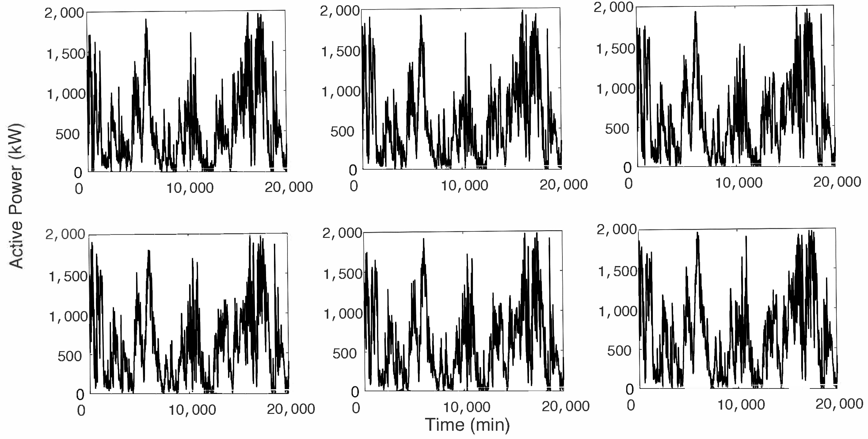
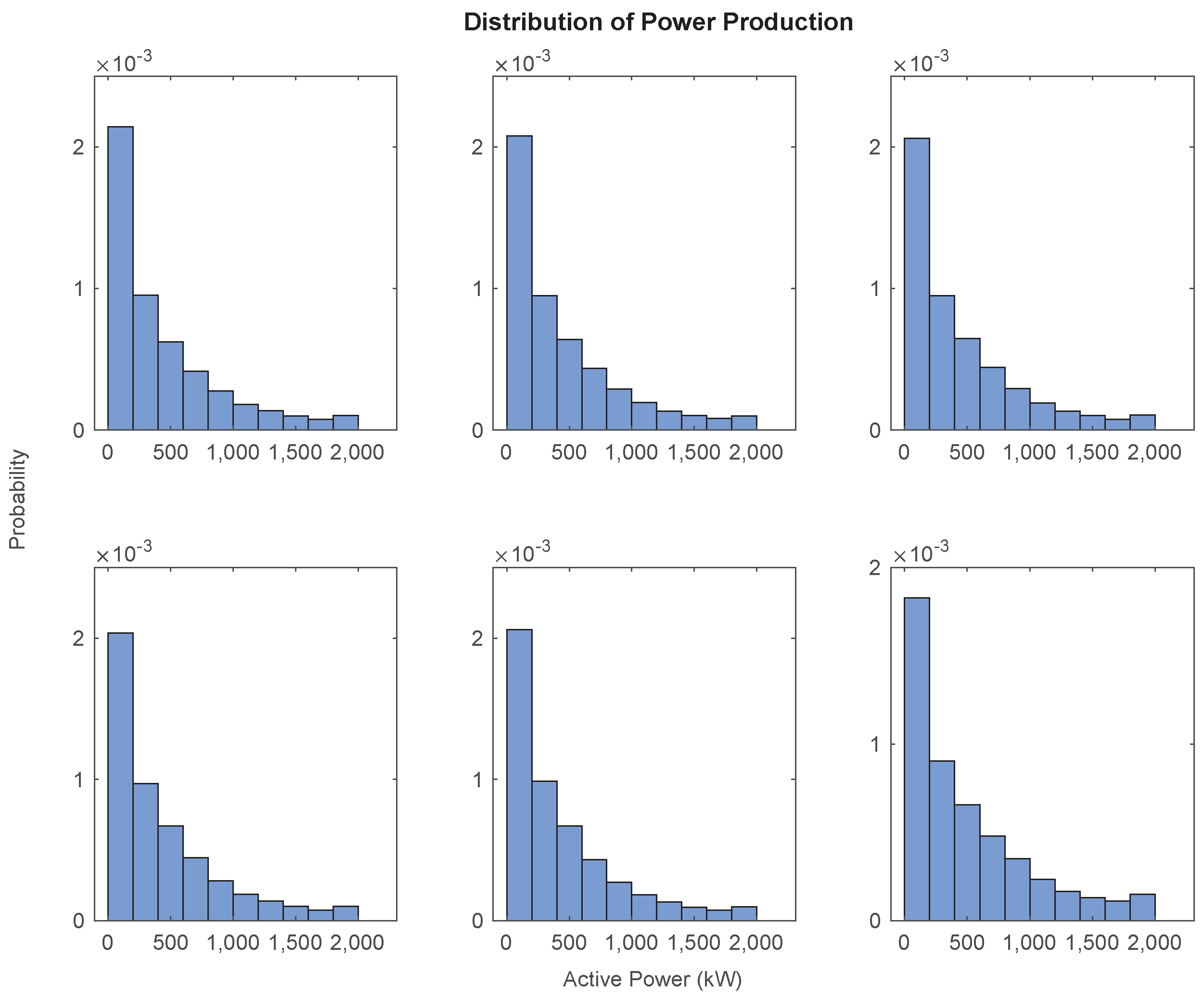
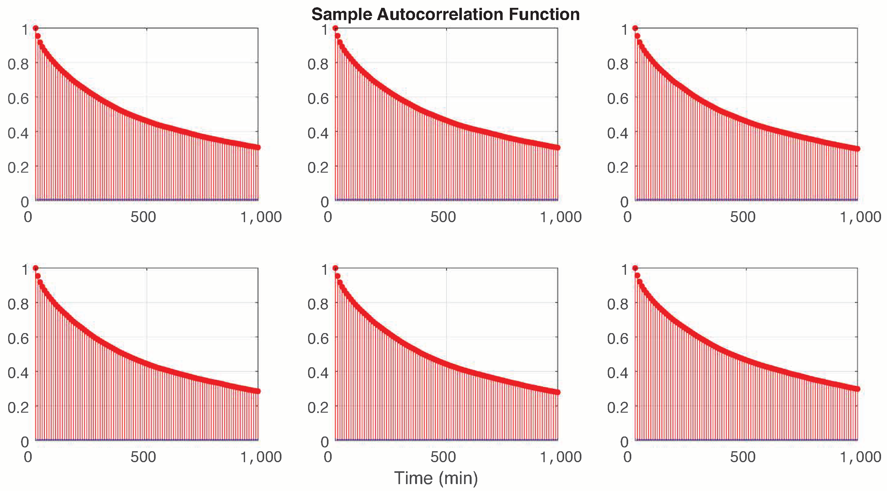
2.1. Dataset

The dataset used in this paper concerns the historical output power (active power) of six wind turbines that constitute a wind farm situated in Poland. The capacity of each turbine is 2 MW. The resolution of data is 10 min, and each output power is an average value over 10 min. The timespan of the data records is 26 months (in the years 2015–2017). The total number of non-missing records is 100,880. Since the wind turbine output powers are the only input to the WPG model, the meteorological knowledge (wind speed and direction, air pressure, ambient temperature, humidity and so on) and information concerning various physical and technical factors (mechanical inertia, pitch control, blades icing, wakes, wind farm layout and many more factors) affecting output power can be neglected. The advantage of this kind of approach is that there is no need to study the stochastic relationships between the output powers and the factors mentioned above.
A sample of the time series of the power produced by the six wind turbines is represented in Figure 1, from which it is possible to see that the WPGs of the six wind turbines share similar temporal behavior.
In Table 1, we show the main statistics concerning the power production for each wind turbine.
Turbines WT1 to WT5 show very similar statistical behaviors: the means and standard deviations are very close to each other and the coefficients of variation (standard deviation over mean) range between 87 % and 90 % . Turbine WT6 exhibits both a higher mean and standard deviation compared to the other turbines. The relative variation, measured using the coefficient of variation, shows a value of 81.6%—the lowest of all the turbines. The values of the skewness show a positive asymmetry for all the turbines; this means that the power distributions have a tail on the right part of the distribution towards large power values. However, the tails are fatter than those of a normal distribution, as documented by the kurtosis values, which are all greater than 3. In Figure 2, we show the empirical distribution functions for each of the six wind turbines.
A striking property of the wind power time series is the presence of a strong autocorrelation; this was already highlighted in previous studies [22] and is also confirmed in our case study by a simple inspection of Figure 3, from which it is possible to see that this function decreases slowly and remains consistently far from zero for all turbines in the wind farm.

2.2. Model

In this section, we first describe the main features of the model used to determine the wind production of each wind turbine and subsequently present the multivariate extension using copula functions. The presentation follows the idea developed in [31], in which a different index process was considered for the appropriate modeling of financial data.

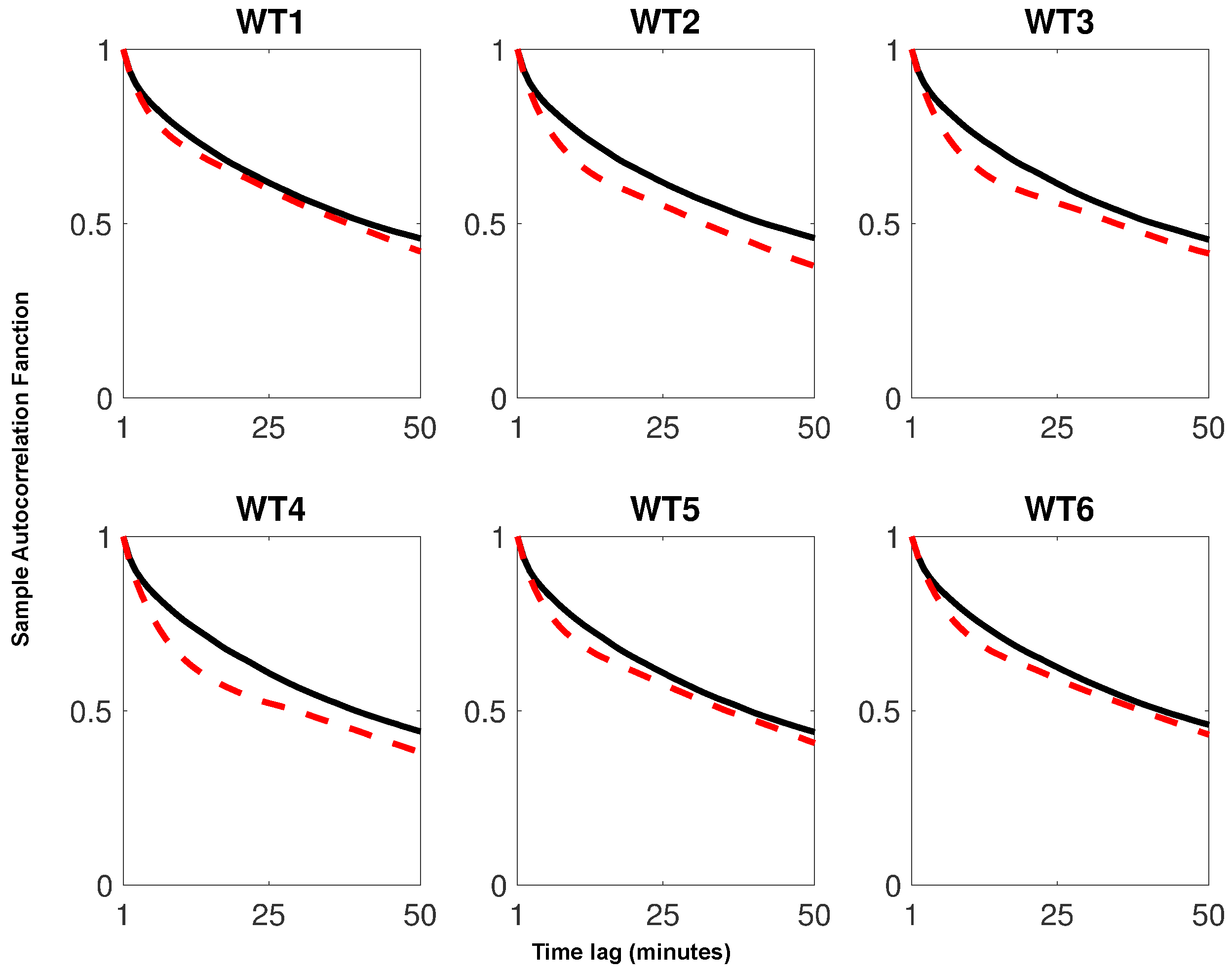
2.2.1. The Indexed Semi-Markov Chain

The wind power production of a single turbine can be modeled faithfully within a semi-Markov framework [22,23,24,26]. Indeed, in the quoted papers, the authors found evidence that a semi-Markov test produces more reliable results compared to the traditional Markov alternative.
In order to cope with the strong autocorrelation in WPG, as shown in Figure 3, we use the more general index semi-Markov model (ISMC hereafter) that was recently introduced by D’Amico and Petroni (see [22,23,24]).
Below, we briefly summarize the main features of the ISMC model (see the work presented in [22,23,24,26] for a detailed survey of the subject).
Semi-Markov processes are an extension of pure Markov processes. Both processes foresee finite states denoted as { v n } with a value in a finite set of E, and the transitions between them are governed through a so-called transition matrix. The specificity of the semi-Markov processes concerns the transition times denoted by { T n } , which follow random variables. In other words, the time that elapses between two consecutive transitions T n + 1 T n may follow any kind of probability distribution function.
As a further improvement of the previous idea, the ISMC model has been used to represent the statistical properties of systems that exhibit a strong autocorrelation, including wind speed and power data [26]. The ISMC is a semi-Markov process with an additional random variable (namely, the index process U) given by the following relation:
U n m = k = 0 m v n 1 k · T n k T n 1 k T n T n 1 m .
The index is a moving average of order m + 1 calculated based on the previous values v n 1 k of the wind power process. We set up the weights as fractions of sojourn times in a given state T n k T n 1 k with respect to the interval length used to compute the average values ( T n T n 1 m ) . In this way, the longer time a system is in a state, the larger the corresponding weight. The main idea is to obtain transition probabilities that depend on many different aspects, such as the last visited state, the sojourn time spent in that state and the value of the index process.
The one-step transition probability matrix can be evaluated by considering the counting transitions between the three random variables considered above. Then, the transition probability matrix P ( t , u ) = { p i , j ( t , u ) } i , j E gives basic probabilities, which are relevant to our work. The generic element p i , j ( t , u ) represents the transition probability from the actual wind power state i to wind power state j, given that the sojourn time spent in the state i is equal to t and the value of the process U m is u. These probabilities can be computed as
p i , j ( t , u ) = n i , j ( t , u ) j n i , j ( t , u ) ,
where n i j ( t , u ) is the total number of transitions observed in the database from state i to state j in the next period, with a sojourn time spent in the wind power i equal to t and a value of the index process equal to u.
The introduction of the index process is useful to cope with the high autocorrelation which is characteristic of wind power series because it allows the differentiation of transition probabilities according to the sample path followed by the wind power process. The parameter m in the index process definition, which is also called memory parameter, should be “optimally” fixed. Indeed, a low value of the memory may not allow the state of the index U m to be established correctly due to a lack of information, whereas a long memory value may overlap with several states, with a consequent loss of information.
According to [26], a viable strategy to calibrate the memory parameter m is to minimize an adequacy indicator such as the mean percentage error (MPE) between the autocorrelation function of the empirical data and the simulated data.
It is worth noting that the ISMC model includes, as a particular case, an important type of stochastic process that is often used in applied problems. Indeed, if transition probabilities p i , j ( t , u ) are independent of u (i.e., the values of p i , j ( t , u ) do not change according to u), we can recover transition probabilities from a semi-Markov model. If p i , j ( t , u ) are independent of the time t, we obtain an indexed Markov chain model [33]. Finally, when p i , j ( t , u ) are independent of both t and u, we recover Markov chain models.

2.2.2. From Univariate to Multivariate Models: The Copula Function Approach

Copula functions are a very general method that allows the representation of multivariate distributions through complex and non-linear dependence structures between marginal distributions; an example is presented in the work by Durante and Sempi [34]. A copula function permits a joint distribution to be split into marginal distributions and a dependence function between them. The copula function contains the dependence structure between the marginal distributions, and the marginal distributions contain other characteristics such as the mean, standard deviation, skewness and kurtosis.
It should be kept in mind that a copula is a multivariate distribution such that its marginals are standard and uniform. A common notation is C u 1 , , u n : [ 0 , 1 ] n [ 0 , 1 ] . The fundamental theorem proved by Sklar [35] states that, given F, a multivariate n-dimensional distribution function with marginals F i , there exists a copula C such that F x 1 , , x n = C F 1 x 1 , , F n x n . The previous relation is the canonical representation of the distribution.
Besides, if the marginals are continuous, then C is unique. For any copula C and marginal distribution function F i , the function
F x 1 , , x n = C F 1 x 1 , , F n x n
defines a multivariate distribution function with marginals F i .
In the previous subsection, we considered an ISMC model for the power production of each wind turbine. Let us denote by ( a ) P ( · , · ) the one-step transition probability matrix that describes the dynamic of power production of the a-th wind turbine. We denoted the corresponding one-step cumulative distribution function by
F ( i a , t a , u a ) ( h a ) = j = i h a ( a ) p i a , j ( t a , u a ) .
This expresses the cumulative distribution function of the power production of turbine a in the next period, which is conditional on the current power production i a , on the sojourn time in this state t a and on the value of the index process u a . We observe here that the cdf of each turbine depends on a specific value of the memory parameter m a , which is not made evident in the notation and contributes to the determination of the matrices ( a ) P ( · , · ) . Then, once a copula function C is fixed, we can obtain a multivariate distribution according to the following relation:
F h 1 , , h k = C F ( i 1 , t 1 , u 1 ) ( h 1 ) , , F ( i k , t k , u k ) ( h k ) .
Function (4) completely describes the wind power production of a wind farm composed of k turbines at the next time period, and thus it is possible to compute any kind of reliability metric.
The choice of the copula function determines the selection of different multivariate models sharing the same fixed marginal distributions obtained applying k different ISMC models—one for each wind turbine. The copula may have parameters that depend on the triplet ( i , t , u ) , or in more simple cases, parameters that remain unchanged in time.

3. Results of Modeling

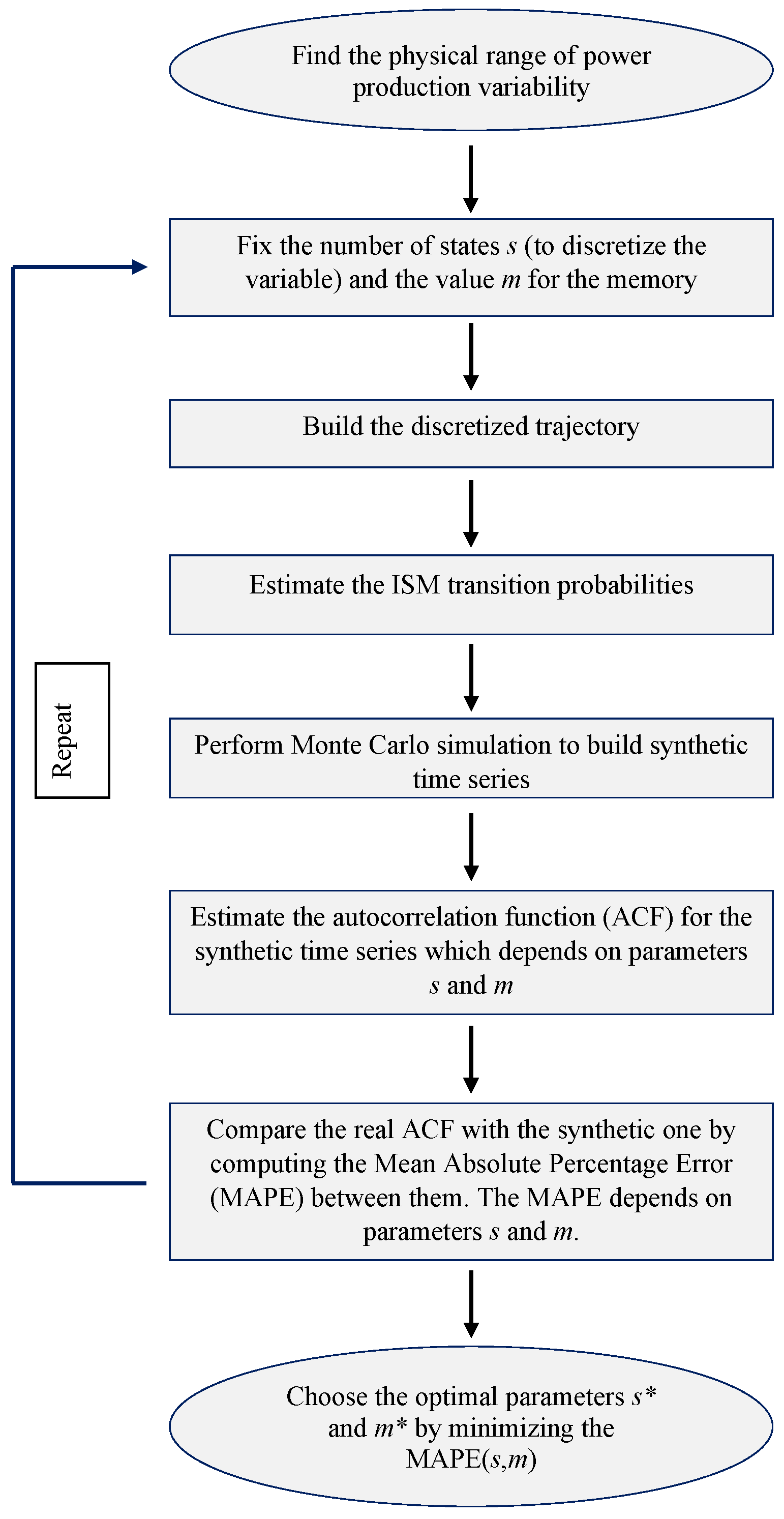
3.1. Parameter Optimization

In order to apply the model, it is necessary to optimize the parameters. The first step is the discretization of the range of values of the wind power. In this application, we used nine states to cover the entire power distribution. The range of each state is reported in Table 2.
The ISMC model epends on the index process defined in ( 1 ) ; therefore, we also discretize the value of this process in order to associate a different transition probability matrix to each state of the index process according to the relation ( 2 ) . In Table 3, we show the selected states of the index process.
We observe that the choice of the states is a fundamental step in this method. It is clear that as the number of states increases, the efficiency of the model improves; on the other hand, the number of parameters to be estimated increases, and the model therefore becomes more expensive in computational terms. A compromise should be found; for more examples of this kind of problem, see [31]. The same problem arises in the choice of the states for the index; this issue was explored in [33].
According to [31,33], we optimized the model parameters m and number of states s by the minimization of a given function. We describe here the whole procedure employed to set and optimize the parameters used in the model.
The first step to set the characteristics of the ISMC model is to determine the physical range of power variability from the empirical data. Next, we fix an arbitrary number of states s to discretize the variable and an arbitrary value for the memory parameter m. After setting these two parameters, we are able to build the discretized trajectory of the process. Afterwards, we estimate the indexed semi-Markov transition probabilities p i j m ( t , u ) . At this point, we know all the structural features of the ISMC process, and we are able to perform a Monte Carlo simulation to build a synthetic time series of power production. This simulated series needs to be compared with the empirical series through the following procedure: first, we estimate the autocorrelation function (ACF) for the synthetic time series Σ ( τ ; s , m ) —note that this ACF depends on the number of states s and on the value of the memory parameter m—then, we compare the real ACF, Σ ( τ ) , with the synthetic ACF, Σ ( τ ; s , m ) , by computing the mean absolute percentage error (MAPE) between them. The MAPE depends on the number of states and on the value of the memory parameter, meaning that it is denoted by M A P E ( s , m ) . At this point, we return to the previous step with other choices for the parameters m and s and repeat the same successive steps.
A brief description of the procedure is illustrated in the flow chart presented in Figure 4.
At the end of the whole process, we choose the number of states s * and memory parameters m * that best represent the dataset by minimizing the MAPE ( s , m ) ; i.e.,
( s * , m * ) = a r g m i n ( s , m ) { MAPE ( s , m ) } .
Note that the algorithm can stop whenever the increase in the number of states does not decrease the MAPE more than a given threshold ϵ .
From the data, the one-step transition probability matrices are estimated according to Formula (2) for each wind turbine. It is worth noting that, if the model is correct, we should have different transition probability matrices according to the values of the index process; i.e., the probability of jumping from one state to another depends on the state occupied by the index process. In formal terms,
p i , j ( t , u ^ ) p i , j ( t , u ˜ ) , for u ^ u ˜ .
To show this, we list in the Appendix A the one-step probability matrices ( a ) P ( 0 ; u ) for turbine a ( a = 1 , , 6 ) and index value u ( u = 1 , 3 , 6 ). We note that these probabilities are significantly different with respect to the turbine considered and especially to the values of the index process. The differences between the transition probability matrices for different values of the index process justify the use of ISMC to model wind power production.
For example, we can compare the probabilities
( 1 ) p 1 , 1 ( 0 , 1 ) = 0.7037 ( 1 ) p 1 , 1 ( 0 , 3 ) = 0.6254 ( 1 ) p 1 , 1 ( 0 , 6 ) = 0.3333 ,
and observe that they express the conditional probability for turbines WT1 to generate a power equal to state 1 (range 0–200 kW) at the next time step conditional on the occupancy at the current time of state 1 (range 0–200 kW) with a duration equal to zero and index process values equal to 1 (range 0–2 MW), 3 (range 3–4 MW) and 6 (range >7 MW), respectively. Thus, the value of the index process acts as a threshold that denotes different dynamics of wind power generation; accordingly, for future power forecasting and management, it is crucial to develop a model that is able to consider this effect.
The results presented in the transition probability matrices are obtained after the calibration of the memory parameter m. In previous papers [26] it has been shown that the optimal value of the memory parameter can be determined by minimizing an adequacy indicator such as the mean percentage error (MPE) between the autocorrelation function of the empirical data and the simulated data.
To this end, in Figure 5, we show the MPE estimated for the autocorrelation functions of empirical and simulated data as a function of the memory value m. The simulated data were obtained by using a Monte Carlo procedure according to [31].
As a consequence, we can deduce that the best memory for each turbine respectively uses m = 8 , 11 , 13 , 15 , 10 , 11 time steps (each time step is 10 min).
In Figure 6, we present a comparison between the empirical autocorrelation and the autocorrelation performed by the model with optimal m values (namely the minimum in Figure 5).
Besides this, the cross-correlation matrix between each pair of power turbines has been computed as follows:
1.0000 0.9517 0.9368 0.9316 0.9279 0.9350 0.9517 1.0000 0.9688 0.9440 0.9338 0.9348 0.9368 0.9688 1.0000 0.9661 0.9429 0.9293 0.9316 0.9440 0.9661 1.0000 0.9616 0.9296 0.9279 0.9338 0.9429 0.9616 1.0000 0.9287 0.9350 0.9348 0.9293 0.9296 0.9287 1.0000
An inspection of the values in matrix ( 6 ) reveals a strong linear dependence between any pair of wind turbines. The correlation coefficients are all greater than 0.92 , which confirms the need to adopt a multivariate model and the inadequacy of considering the different turbines as independent from each other.
Another justification of using a multivariate model is given by the difference between the variance of the total power production processes, which is 7.6 × 10 6 , and the sum of the variance of each turbine, which is instead 1.26 × 10 6 due to the high correlation between the different turbines.
To represent the complex dependence structure between wind turbines, we used and compared several copulas, such as the Gumbel copula, which belongs to the important class of Archimedean copulas, the Gaussian copula and finally the t-Student copula with different degrees of freedom. The Gumbel copula has been included because it is able to maintain the tail dependence on one side of the distribution. To estimate the parameters of the copulas, we applied the inference functions for margins (IFM) method which foresees the classical maximization of the log-likelihood functions [36]. Besides, random number generators from copulas are available within Matlab toolboxes or other software.

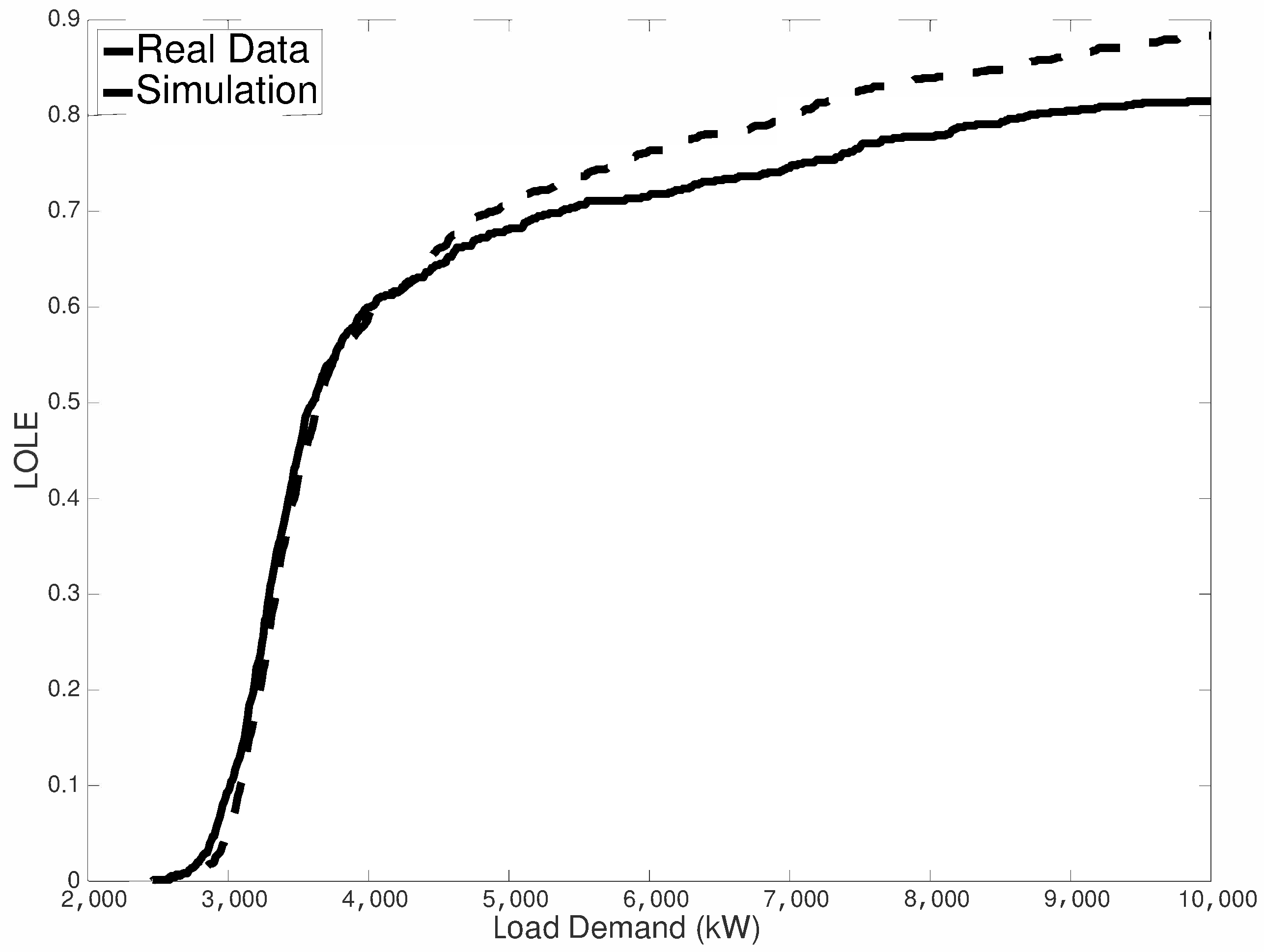
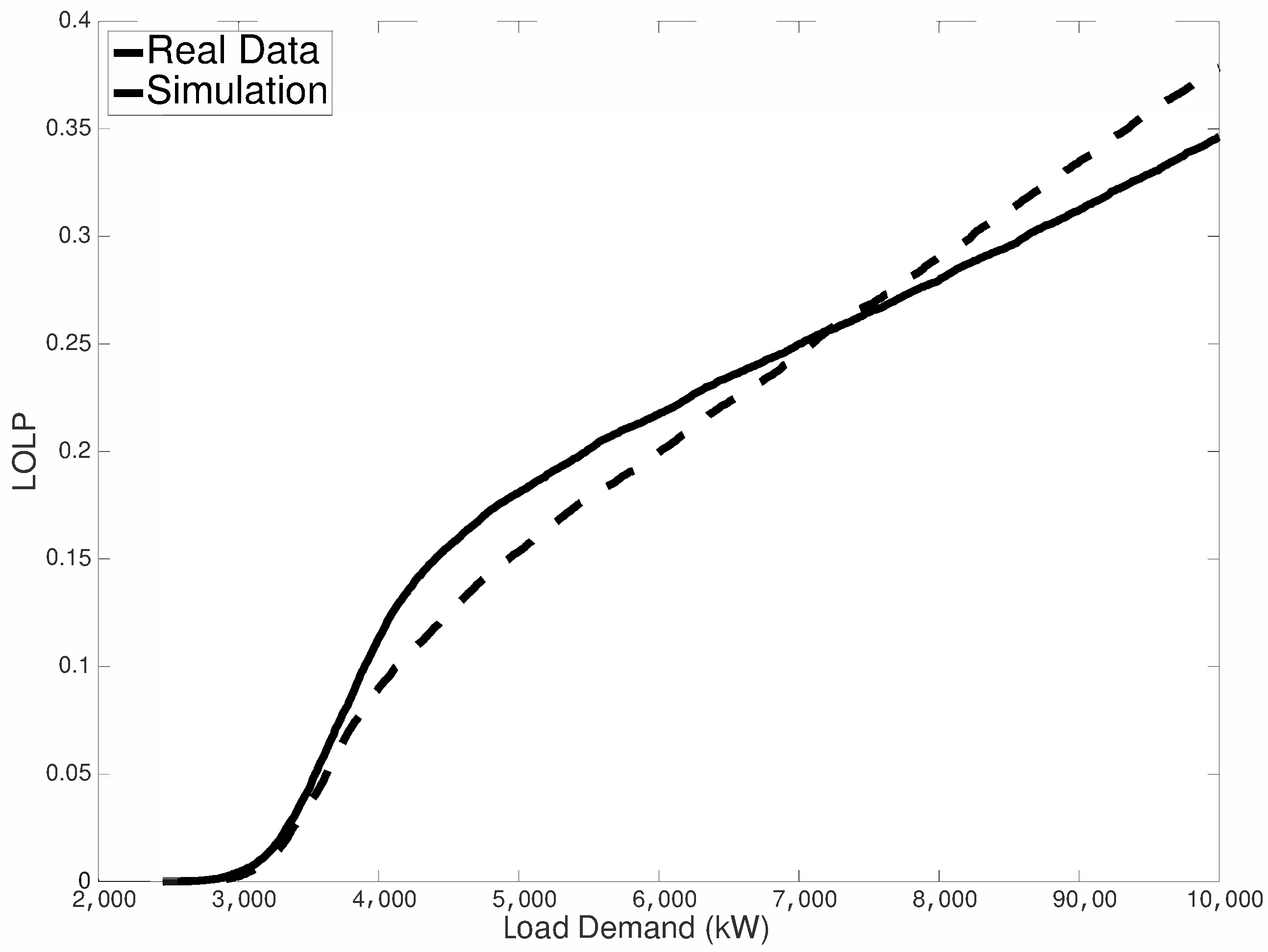
3.2. Estimation of Reliability Indices

To show the accuracy of the proposed model, we present the results of the estimation of some reliability indices [37] commonly used in the analysis of the adequacy of power generation; i.e., loss of load hours, loss of load expectation and loss of load probability. We evaluate these indices based on both real and simulated data to highlight the accuracy of our model. We assume the load demand level is assigned to one value for any point in time (constant value) ranging between 2500 and 10,000 kW.

3.2.1. Loss of Load Hours

The loss of load hours (LOLH) index represents the expected number of hours per period (typically one year) in which a system’s demand exceeds the generating capacity.
The LOLH is estimated according to the following procedure:
  • Fix the length of the period H;
  • By means of a Monte Carlo algorithm, generate N trajectories of the power produced by the wind farm according to the multivariate ISMC model with the same initial conditions. More specifically, the data can be described in the form of an array:
    z 11 z 12 z 1 H z 21 z 22 z 2 H z N 1 z N 2 z N H
    where z i j is the energy produced by the wind farm (generating capacity) at time j in the i th simulation. We introduce the notation z i · : = z i 1 , , z i H with i = 1 , 2 , , N and observe that the z i · i = 1 N are N independent realizations of the same stochastic process.
  • Convert the array in a 0–1 array according to whether the system’s demand at the time j, S D j exceeds the generating capacity z k j in the considered simulation. This can be expressed as follows:
    I k j = 1 if S D j > z k j 0 otherwise
  • Let L O L H k = j = 1 H I k j denote the number of hours in which the demand is not supplied. The sequence L O L H k k = 1 N is a random sample of size N because the random variables L O L H k are mutually independent and identically distributed according to the simulation scheme in step 2. Estimate the LOLH using the sample mean; i.e.,
    L O L ^ H = k = 1 N L O L H k N
    and denote by
    S L D ^ H = 1 N 1 k = 1 N L O L H k L O L ^ H 2
    the sample variance. From basic statistical inference, we know that estimates (8) and (9) are unbiased, and for large N, due to the central limit theorem, we can construct confidence intervals for the LOLH at a given significance level α :
    C I ( 1 α ) = L O L ^ H ± z α / 2 · S L D ^ H
    where ± z α / 2 are the critical values at the level α of a normal standard distribution.
In Figure 7, we show the estimation of LOLH for both empirical and simulated data as a function of the load demand. We considered here a dependence structure given by the t-Student copula with 10 degrees of freedom (which represents the best choice, as will be shown below). It can be seen that there is a good agreement between the two curves in the plot, and the estimated MAPE is equal to 8.32 % . In more detail, this figure shows the appropriateness of our model for describing wind power generation. It is important to note that, for both small and large values of the system’s demand—i.e., values in the ranges of 2500–4000 kW and 7000–10,000 kW—there is a very good agreement between real and simulated data. This means that if we need to forecast the LOLH for those ranges, the model is able to provide very accurate predictions. The performance of the model decreases slightly in relation to the medium system’s demand (4000–7000 kW), where the model provides again good results. In fact, the maximum difference of about 250 h between real and simulated data is obtained for a system demand approximately equal to 5000 kW. This difference means that in one year (8760 h) our model disagrees with real data by only 250 h, with a low defeat rate equal to 250 8760 = 2.85 % . Thus, in the worst case (a system demand equal to 5000 kW), the model can predict LOLH in 97.15% of cases.

3.2.2. Loss of Load Expectation

The loss of load expectation (LOLE) gives the expected number of days per period (typically a year) for which the available generation capacity is insufficient to serve the demand at least once per day. Therefore, LOLE counts the days which experience loss of load events, regardless of the number of consecutive or nonconsecutive loss of load hours in the day.
The LOLE is estimated according to the following procedure, in which the first three steps coincide with those used for the LOLH estimation:
Let D be the number of days in the considered period. For all d = 1 , , D and k = 1 , , N define
E k , d = 1 if i = 1 24 I k i 0 0 otherwise
and compute
L O L E k : = d = 1 D E k , d D
According to the simulation scheme described above, we obtain a sequence L O L E k k = 1 N of i.i.d. random variables, and its sample mean is an estimator of the LOLE, namely
L O L ^ E : = k = 1 N L O L E k N
The estimator L O L ^ E is unbiased (for the basic statistical inference, see for example the work in [38]), and once we estimate the sample variance by means of
S L O L ^ E = 1 N 1 k = 1 N L O L E k L O L ^ E 2 ,
we can construct confidence intervals to any significant level α as previously performed for the LOLH.
Results for this indicator are shown in Figure 8. In this case, the estimated MAPE is equal to 4.88 % , showing a very good agreement between empirical and simulated values.

3.2.3. Loss of Load Probability

The loss of load probability (LOLP) represents the probability of the system’s daily peak or hourly demand exceeding the available generating capacity during a given period. We can estimate this probability either using only the daily peak loads (or the daily peak variation curve) or all the hourly loads (or the load duration curve) for each period considered. The calculation with the Monte Carlo procedure is able to sample from the available generation potential and demand distributions and to repeat the process to determine how many times a loss of load will occur. Then, LOLP represents the number of loss of load events divided by the number of sample simulations.
In our application, the LOLP is given by the LOLH in the whole period divided by the number of hours in the same period. Then, we can perform estimation using the same procedure used for LOLH. The results are shown in Figure 9. In this case, there is a good agreement between simulated and empirical estimations with a MAPE of 7.23%.
To complete our analysis, we considered and compared the dependency structure modeled by the categories of copula functions listed above; specifically, the Student copula (with 2, 6, 8, 10 and 20 degrees of freedom) and the Gaussian copula. Finally, we compared our model with a typical process used in econometric modeling, namely the VAR (vector autoregressive model). In our case, we applied a V A R ( 6 , 2 ) with six variables (corresponding to the production of each individual wind turbine) and two lags. For the choice of optimal lags, we took into account the criteria based on the AIC and BIC indicators, and we verified the significance of the parameters. For the sake of brevity, we omit the values of the estimated parameters. Finally, in Table 4 below, we report the results of the different models that we can compare using the MAPE. We note that the best results are obtained with the ISMC- t 10 copula model, while the VAR model produces a significantly lower adaptation.

4. Discussion

Based on previous research works in which the suitability of a semi-Markovian approach to generate synthetic time series of wind speed was confirmed, in this research, we apply the indexed semi-Markov chain (ISMC) model to model the energy produced by a whole wind farm. To this end, the ISMC model has been extended to a multivariate setting in which each marginal represents the energy produced by a wind turbine in a wind farm. The model, by means of Monte Carlo simulations, has been compared with real data from a wind farm in Poland. We have shown that the model is able to reproduce the statistical properties of univariate and multivariate real data. Given these results, the model has been used to estimate different risk metrics that are usually used in resource adequacy planning; more specifically, we estimated the loss of load hours, loss of load expectation and loss of load probability from real and simulated data, showing a very good agreement and predictive power.
Future works will focus on the development of the statistical estimation of the reliability indicators (LOLE, LOLH and LOLP). This is an important task that will provide asymptotic confidence intervals for the aforementioned indicators.

Author Contributions

Conceptualization, G.D. and F.P.; Data curation, G.M. and R.A.S.; Formal analysis, G.M.; Methodology, G.D. and F.P.; Software, F.P.; Supervision, G.D. and F.P.; Validation, R.A.S. All authors have read and agreed to the published version of the manuscript.

Funding

This research received no external funding.

Conflicts of Interest

The authors declare no conflict of interest.

Appendix A

Here, we list the one-step probability matrices ( a ) P ( 0 ; u ) for turbine a ( a = 1 , , 6 ) and index value u ( u = 1 , 3 , 6 ).
( 1 ) P ( 0 ; 1 ) = 0.7037 0.2838 0.0117 0.0014 0.0005 0.0000 0.0000 0.0000 0.0000 0.2603 0.6268 0.0983 0.0104 0.0025 0.0006 0.0000 0.0006 0.0006 0.0213 0.3221 0.4989 0.1240 0.0242 0.0051 0.0015 0.0015 0.0015 0.0062 0.0871 0.3070 0.4460 0.1100 0.0249 0.0124 0.0021 0.0041 0.0176 0.0059 0.1353 0.3177 0.3059 0.1529 0.0588 0.0058 0.0000 0.0126 0.0000 0.0759 0.1392 0.2911 0.3165 0.1266 0.0127 0.0253 0.0263 0.0526 0.0263 0.1053 0.1316 0.2895 0.1842 0.0789 0.1053 0.0000 0.0909 0.0000 0.0909 0.0909 0.2727 0.0909 0.0909 0.2723 0.0833 0.0000 0.0000 0.0000 0.0000 0.0000 0.3333 0.0833 0.5000 ;
( 1 ) P ( 0 ; 3 ) = 0.6254 0.3158 0.0464 0.0093 0.0000 0.0000 0.0031 0.0000 0.0000 0.0935 0.6146 0.2434 0.0344 0.0079 0.0035 0.0009 0.0009 0.0009 0.0080 0.1934 0.5484 0.2050 0.0306 0.0086 0.0012 0.0037 0.0012 0.0007 0.0389 0.2725 0.4968 0.1585 0.0226 0.0057 0.0021 0.0021 0.0037 0.0224 0.0997 0.3142 0.3865 0.1484 0.0212 0.0025 0.0012 0.0031 0.0031 0.0220 0.1352 0.2925 0.3616 0.1226 0.0440 0.0157 0.0099 0.0099 0.0198 0.0693 0.1287 0.3960 0.2376 0.0792 0.0495 0.0000 0.0000 0.0217 0.0867 0.1304 0.1522 0.2174 0.2391 0.1523 0.0000 0.0000 0.0000 0.0000 0.0323 0.0645 0.0645 0.2903 0.5484 ;
( 1 ) P ( 0 ; 6 ) = 0.3333 0.2222 0.0000 0.2222 0.1111 0.1111 0.0000 0.0000 0.0000 0.0625 0.4375 0.2500 0.0625 0.0625 0.0000 0.0000 0.0000 0.1250 0.0189 0.1698 0.2076 0.3396 0.0755 0.0755 0.0943 0.0000 0.0189 0.0074 0.0370 0.1556 0.3333 0.2667 0.1037 0.0444 0.0296 0.0222 0.0000 0.0068 0.0273 0.1536 0.3686 0.2526 0.1297 0.0341 0.0273 0.0000 0.0021 0.0123 0.0534 0.2156 0.3593 0.2320 0.0801 0.0452 0.0000 0.0014 0.0057 0.0187 0.0647 0.1968 0.3764 0.2098 0.1264 0.0000 0.0000 0.0000 0.0014 0.0257 0.0851 0.2284 0.3932 0.2662 0.0000 0.0000 0.0000 0.0020 0.0040 0.0375 0.1067 0.2549 0.5949 ;
( 2 ) P ( 0 ; 1 ) = 0.6983 0.2871 0.0112 0.0021 0.0011 0.0005 0.0000 0.0000 0.0000 0.2507 0.6126 0.1202 0.0126 0.0026 0.0003 0.0003 0.0000 0.0007 0.0219 0.3133 0.5041 0.1313 0.0185 0.0055 0.0007 0.0021 0.0027 0.0036 0.0700 0.3393 0.4452 0.1077 0.0179 0.0126 0.0036 0.0000 0.0051 0.0204 0.1122 0.3520 0.3316 0.1327 0.0357 0.0102 0.0000 0.0130 0.0390 0.0390 0.1169 0.2597 0.2987 0.1299 0.0390 0.0649 0.0000 0.0000 0.0588 0.0882 0.2647 0.3529 0.2059 0.0000 0.0294 0.0000 0.0000 0.0000 0.0000 0.1667 0.1667 0.3333 0.1667 0.1667 0.0000 0.0667 0.0000 0.0000 0.0000 0.1333 0.0667 0.2667 0.4667 ;
( 2 ) P ( 0 ; 3 ) = 0.6639 0.3034 0.0109 0.0055 0.0109 0.0027 0.0000 0.0000 0.0027 0.0974 0.6200 0.2304 0.0409 0.0061 0.0026 0.0009 0.0017 0.0000 0.0074 0.1879 0.5669 0.1947 0.0283 0.0111 0.0025 0.0012 0.0000 0.0029 0.0399 0.2773 0.4818 0.1661 0.0235 0.0057 0.0014 0.0014 0.0037 0.0147 0.0846 0.2978 0.4289 0.1336 0.0270 0.0049 0.0049 0.0028 0.0056 0.0306 0.1472 0.2944 0.3444 0.1139 0.0444 0.0167 0.0065 0.0000 0.0130 0.0455 0.1688 0.3117 0.2857 0.1234 0.0455 0.0000 0.0270 0.0270 0.0540 0.0676 0.1216 0.2432 0.2297 0.2297 0.0000 0.0000 0.0000 0.0000 0.05556 0.055 0.1944 0.3889 0.3056 ;
( 2 ) P ( 0 ; 6 ) = 0.0000 0.2500 0.0000 0.2500 0.2500 0.0000 0.0000 0.2500 0.0000 0.0714 0.7143 0.2143 0.0000 0.0000 0.0000 0.0000 0.0000 0.0000 0.0152 0.1818 0.3939 0.2273 0.1364 0.0303 0.0152 0.0000 0.0000 0.0000 0.0140 0.1958 0.3497 0.2587 0.1329 0.0140 0.0280 0.0070 0.0035 0.0070 0.0317 0.1585 0.3803 0.2642 0.1056 0.0317 0.0176 0.0022 0.0022 0.0108 0.0626 0.2052 0.3737 0.2613 0.0583 0.0238 0.0000 0.0000 0.0017 0.0217 0.0619 0.2291 0.3462 0.2542 0.0853 0.0000 0.0000 0.0029 0.0058 0.0173 0.0794 0.2121 0.3939 0.2886 0.0022 0.0000 0.0000 0.0044 0.0088 0.0396 0.0661 0.2335 0.6454 ;
( 3 ) P ( 0 ; 1 ) = 0.7062 0.2748 0.0152 0.0022 0.0000 0.0011 0.0005 0.0000 0.0000 0.2351 0.6182 0.1278 0.0151 0.0024 0.0003 0.0007 0.0003 0.0000 0.0235 0.3161 0.5029 0.1221 0.0255 0.0046 0.0026 0.0013 0.0013 0.0050 0.0448 0.3383 0.4229 0.1410 0.0332 0.0099 0.0033 0.0017 0.0082 0.0206 0.1563 0.3416 0.2922 0.1482 0.0206 0.0041 0.0082 0.0000 0.0326 0.0645 0.1398 0.3226 0.3011 0.0645 0.0430 0.0323 0.0000 0.0714 0.0476 0.0714 0.1190 0.2143 0.2857 0.0952 0.0952 0.0000 0.0000 0.0588 0.0588 0.0588 0.2353 0.3529 0.1765 0.0588 0.0769 0.0000 0.0000 0.0769 0.0000 0.1539 0.0769 0.2308 0.3846 ;
( 3 ) P ( 0 ; 3 ) = 0.6427 0.3251 0.0149 0.0099 0.0000 0.0074 0.0000 0.0000 0.0000 0.0950 0.6096 0.2491 0.0299 0.0103 0.0017 0.0017 0.0017 0.0009 0.0081 0.1814 0.5756 0.1962 0.0271 0.0086 0.0012 0.0012 0.0006 0.0036 0.0384 0.2710 0.5007 0.1507 0.0297 0.0029 0.0029 0.0000 0.0000 0.0134 0.0782 0.3178 0.4120 0.1345 0.0330 0.0073 0.0037 0.0026 0.0000 0.0130 0.1143 0.3272 0.3325 0.1455 0.0442 0.0208 0.0000 0.0123 0.0123 0.0613 0.0982 0.3251 0.2883 0.1595 0.0429 0.0000 0.0115 0.0000 0.0345 0.0575 0.1149 0.2759 0.3104 0.1954 0.0392 0.0000 0.0000 0.0000 0.0196 0.0588 0.1569 0.2549 0.4706 ;
( 3 ) P ( 0 ; 6 ) = 0.5000 0.1667 0.0000 0.0000 0.1667 0.1667 0.0000 0.0000 0.0000 0.0952 0.5238 0.2857 0.0476 0.0476 0.0000 0.0000 0.0000 0.0000 0.0141 0.1409 0.3803 0.2676 0.0704 0.0423 0.0282 0.0141 0.0423 0.0000 0.0245 0.1288 0.3988 0.2761 0.0798 0.0614 0.0123 0.0184 0.0000 0.0032 0.0508 0.2000 0.3778 0.2349 0.0476 0.0571 0.0286 0.0023 0.0023 0.0183 0.0550 0.1949 0.3899 0.2087 0.0940 0.0344 0.0000 0.0000 0.0018 0.0071 0.0724 0.2332 0.3657 0.2156 0.1042 0.0000 0.0000 0.0031 0.0046 0.0201 0.0849 0.2253 0.3812 0.2809 0.0000 0.0000 0.0000 0.0024 0.0214 0.0238 0.0786 0.2738 0.6000 ;
( 4 ) P ( 0 ; 1 ) = 0.6959 0.2842 0.0154 0.0028 0.0011 0.0000 0.0006 0.0000 0.0000 0.2369 0.6238 0.1202 0.0139 0.0028 0.0010 0.0003 0.0007 0.0003 0.0182 0.3070 0.5098 0.1356 0.0202 0.0039 0.0033 0.0006 0.0013 0.0091 0.0456 0.3394 0.4171 0.1446 0.0350 0.0076 0.0015 0.0000 0.0081 0.0122 0.0979 0.3592 0.3184 0.1592 0.0408 0.0040 0.0000 0.0000 0.0090 0.0721 0.1712 0.2703 0.2793 0.1441 0.0270 0.0270 0.0185 0.0185 0.0185 0.0741 0.1852 0.2407 0.2407 0.1111 0.0926 0.0000 0.0000 0.0000 0.0500 0.0000 0.4000 0.3000 0.1000 0.1500 0.0833 0.0000 0.0000 0.0000 0.0000 0.1667 0.0833 0.3333 0.3333 ;
( 4 ) P ( 0 ; 3 ) = 0.6430 0.3192 0.0236 0.0047 0.0024 0.0024 0.0047 0.0000 0.0000 0.0999 0.6435 0.2159 0.0229 0.0118 0.0034 0.0017 0.0000 0.0008 0.0102 0.1925 0.5616 0.1881 0.0330 0.0127 0.0019 0.0000 0.0000 0.0046 0.0398 0.2603 0.5069 0.1554 0.0260 0.0031 0.0023 0.0015 0.0012 0.0087 0.0798 0.3030 0.4115 0.1571 0.0224 0.0112 0.0050 0.0025 0.0025 0.0254 0.0990 0.3173 0.3579 0.1447 0.0406 0.0102 0.0056 0.0000 0.0056 0.0449 0.1181 0.2528 0.3483 0.1854 0.0393 0.0107 0.0108 0.0000 0.0538 0.0538 0.1505 0.3118 0.2366 0.1720 0.0000 0.0000 0.0000 0.0208 0.0000 0.1667 0.1042 0.1875 0.5208 ;
( 4 ) P ( 0 ; 6 ) = 0.3636 0.1818 0.0000 0.0909 0.1818 0.0000 0.0000 0.0000 0.1818 0.1429 0.5238 0.2381 0.0476 0.0476 0.0000 0.0000 0.0000 0.0000 0.0380 0.1139 0.4177 0.2911 0.1139 0.0253 0.0000 0.0000 0.0000 0.0000 0.0114 0.2114 0.3543 0.2629 0.1314 0.0114 0.0000 0.0171 0.0000 0.0066 0.0364 0.2185 0.4106 0.2053 0.0828 0.0331 0.0066 0.0000 0.0023 0.0069 0.0437 0.2506 0.3678 0.2322 0.0690 0.0276 0.0019 0.0000 0.0037 0.0130 0.0779 0.2189 0.3655 0.2226 0.0965 0.0000 0.0000 0.0000 0.0035 0.0105 0.0773 0.2430 0.3814 0.2777 0.0027 0.0000 0.0000 0.0055 0.0000 0.0354 0.1090 0.2752 0.5722 ;
( 5 ) P ( 0 ; 1 ) = 0.7045 0.2759 0.0140 0.0036 0.0005 0.0000 0.0005 0.0000 0.0005 0.2398 0.6387 0.1049 0.0127 0.0013 0.0016 0.0007 0.0000 0.0003 0.0181 0.3085 0.5380 0.1101 0.0145 0.0065 0.0022 0.0007 0.0014 0.0039 0.0631 0.3491 0.4300 0.1164 0.0237 0.0118 0.0020 0.0000 0.0176 0.0294 0.1059 0.3177 0.3235 0.1588 0.0353 0.0059 0.0059 0.0128 0.0128 0.0641 0.1410 0.2821 0.2564 0.1539 0.0128 0.0641 0.0526 0.0526 0.0263 0.1316 0.1842 0.2105 0.2633 0.0789 0.0000 0.0000 0.0000 0.0000 0.0714 0.0714 0.2857 0.2143 0.1429 0.2143 0.0667 0.0000 0.0000 0.0000 0.2000 0.0667 0.0000 0.2000 0.4667 ;
( 5 ) P ( 0 ; 3 ) = 0.5961 0.3531 0.0367 0.0085 0.0029 0.0000 0.0028 0.0000 0.0000 0.0888 0.6157 0.2348 0.0436 0.0102 0.0051 0.0017 0.0000 0.0000 0.0072 0.1700 0.5769 0.2004 0.0317 0.0102 0.0012 0.0012 0.0012 0.0028 0.0355 0.2498 0.5080 0.1580 0.0362 0.0077 0.0007 0.0014 0.0037 0.0137 0.0974 0.3333 0.3658 0.1336 0.0350 0.0150 0.0025 0.0028 0.0056 0.0280 0.1429 0.3417 0.2913 0.1204 0.0420 0.0252 0.0081 0.0081 0.0161 0.0887 0.1855 0.2258 0.2742 0.1452 0.0484 0.0000 0.0000 0.0000 0.0571 0.1286 0.1286 0.2571 0.2714 0.1571 0.0000 0.0000 0.0000 0.0000 0.0000 0.0645 0.1936 0.1936 0.5484 ;
( 5 ) P ( 0 ; 6 ) = 0.3750 0.2500 0.1250 0.2500 0.0000 0.0000 0.0000 0.0000 0.0000 0.2000 0.4500 0.1000 0.1500 0.0500 0.0500 0.0000 0.0000 0.0000 0.0000 0.1200 0.4800 0.2000 0.0800 0.0600 0.0000 0.0000 0.0600 0.0000 0.0486 0.1944 0.3125 0.2431 0.0903 0.0556 0.0347 0.0208 0.0038 0.0038 0.0263 0.1278 0.4323 0.2293 0.0902 0.0564 0.0301 0.0000 0.0042 0.0126 0.0693 0.1681 0.3508 0.2668 0.0924 0.0357 0.0016 0.0032 0.0032 0.0147 0.0648 0.2366 0.4003 0.1865 0.0891 0.0015 0.0000 0.0000 0.0061 0.0289 0.0746 0.2207 0.3866 0.2816 0.0024 0.0024 0.0024 0.0000 0.0071 0.0449 0.0733 0.2506 0.6170 ;
( 6 ) P ( 0 ; 1 ) = 0.7016 0.2837 0.0120 0.0013 0.0007 0.0000 0.0008 0.0000 0.0000 0.2416 0.6251 0.1167 0.0130 0.0028 0.0000 0.0008 0.0000 0.0000 0.0165 0.3100 0.5374 0.1133 0.0157 0.0071 0.0000 0.0000 0.0000 0.0064 0.0382 0.3248 0.4522 0.1359 0.0340 0.0042 0.0000 0.0042 0.0057 0.0230 0.0805 0.3103 0.3793 0.1379 0.0460 0.0057 0.0115 0.0247 0.0123 0.0123 0.1358 0.2346 0.3457 0.1605 0.0370 0.0370 0.0303 0.0000 0.0000 0.0303 0.2121 0.2424 0.2727 0.1212 0.0909 0.0000 0.0000 0.0000 0.0000 0.0714 0.1429 0.3571 0.1429 0.2857 0.0000 0.0000 0.0000 0.0000 0.0000 0.1000 0.3000 0.1000 0.5000 ;
( 6 ) P ( 0 ; 3 ) = 0.6658 0.2995 0.0224 0.0074 0.0028 0.0025 0.0000 0.0000 0.0000 0.1026 0.6231 0.2316 0.0342 0.0043 0.0026 0.0000 0.0017 0.0000 0.0108 0.1960 0.5568 0.1942 0.0325 0.0072 0.0018 0.0006 0.0000 0.0040 0.0286 0.2679 0.4887 0.1670 0.0314 0.0102 0.0014 0.0007 0.0022 0.0112 0.0694 0.2844 0.4390 0.1601 0.0269 0.0045 0.0022 0.0023 0.0091 0.0227 0.1023 0.3068 0.3864 0.1114 0.0295 0.0295 0.0000 0.0055 0.0220 0.0714 0.1374 0.3187 0.2527 0.1429 0.0494 0.0000 0.0000 0.0000 0.0241 0.1205 0.1325 0.2530 0.2771 0.1928 0.0196 0.0196 0.0000 0.0000 0.0000 0.0588 0.1372 0.1961 0.5686 ;
( 6 ) P ( 0 ; 6 ) = 0.6250 0.0000 0.1250 0.1250 0.0000 0.0000 0.1250 0.0000 0.0000 0.0476 0.4762 0.2381 0.0952 0.0000 0.0000 0.0952 0.0000 0.0476 0.0135 0.1486 0.3243 0.3108 0.1351 0.0270 0.0135 0.0135 0.0135 0.0054 0.0270 0.1568 0.3784 0.2919 0.0703 0.0162 0.0162 0.0378 0.0027 0.0027 0.0326 0.1766 0.3940 0.2554 0.0679 0.0380 0.0299 0.0000 0.0032 0.0080 0.0513 0.1894 0.3868 0.2360 0.0931 0.0321 0.0024 0.0000 0.0036 0.0228 0.0529 0.2344 0.3606 0.2163 0.1070 0.0000 0.0010 0.0000 0.0052 0.0147 0.0651 0.2413 0.3641 0.3085 0.0015 0.0000 0.0015 0.0015 0.0073 0.0248 0.0918 0.2551 0.6166 .

References

  1. Choi, S.; Kim, S. An investigation of operating behavior characteristics of a wind power system using a fuzzy clustering method. Expert Syst. Appl. 2017, 81, 244–250. [Google Scholar] [CrossRef]
  2. Papaefthymiou, G.; Kurowicka, D. Using copulas for modeling stochastic dependence in power system uncertainty analysis. IEEE Trans. Power Syst. 2008, 24, 40–49. [Google Scholar] [CrossRef] [Green Version]
  3. Song, Z.; Geng, X.; Kusiak, A.; Xu, C. Mining markov chain transition matrix from wind speed time series data. Expert Syst. Appl. 2011, 38, 10229–10239. [Google Scholar] [CrossRef]
  4. Salcedo-Sanz, S.; Ortiz-Garcı, E.G.; Pérez-Bellido, Á.M.; Portilla-Figueras, A.; Prieto, L. Short term wind speed prediction based on evolutionary support vector regression algorithms. Expert. Appl. 2011, 38, 4052–4057. [Google Scholar] [CrossRef]
  5. Chang, T.P. Estimation of wind energy potential using different probability density functions. Appl. Energy 2011, 88, 1848–1856. [Google Scholar] [CrossRef]
  6. Chang, T.P. Performance comparison of six numerical methods in estimating weibull parameters for wind energy application. Appl. Energy 2011, 88, 272–282. [Google Scholar] [CrossRef]
  7. D’Amico, G.; Petroni, F.; Prattico, F. Economic performance indicators of wind energy based on wind speed stochastic modeling. Appl. Energy 2015, 154, 290–297. [Google Scholar] [CrossRef]
  8. Danao, L.A.; Eboibi, O.; Howell, R. An experimental investigation into the influence of unsteady wind on the performance of a vertical axis wind turbine. Appl. Energy 2013, 107, 403–411. [Google Scholar] [CrossRef]
  9. Nagai, B.M.; Ameku, K.; Roy, J.N. Performance of a 3kw wind turbine generator with variable pitch control system. Appl. Energy 2009, 86, 1774–1782. [Google Scholar] [CrossRef]
  10. Villanueva, D.; Feijóo, A.; Pazos, J.L. Simulation of correlated wind speed data for economic dispatch evaluation. IEEE Trans. Sustain. Energy 2012, 3, 142–149. [Google Scholar] [CrossRef]
  11. Zhang, Y.; Wang, J.; Wang, X. Review on probabilistic forecasting of wind power generation. Renew. Sustain. Energy Rev. 2014, 32, 255–270. [Google Scholar] [CrossRef]
  12. Ambach, D. Short-term wind speed forecasting in germany. J. Appl. Stat. 2016, 43, 351–369. [Google Scholar] [CrossRef] [Green Version]
  13. Iman, R.L.; Conover, W.J. A distribution-free approach to inducing rank correlation among input variables. Commun. Stat. Simul. Comput. 1982, 11, 311–334. [Google Scholar] [CrossRef]
  14. Morales, J.M.; Mínguez, R.; Conejo, A.J. A methodology to generate statistically dependent wind speed scenarios. Appl. Energy 2010, 87, 843–855. [Google Scholar] [CrossRef]
  15. Yunus, K.; Chen, P.; Thiringer, T. Modelling spatially and temporally correlated wind speed time series over a large geographical area using varma. IET Renew. Power Gener. 2017, 11, 132–142. [Google Scholar] [CrossRef]
  16. D’Amico, G.; Petroni, F.; Prattico, F. Wind speed prediction for wind farm applications by extreme value theory and copulas. J. Wind Eng. Ind. Aerodyn. 2015, 145, 229–236. [Google Scholar] [CrossRef]
  17. Hu, W.; Min, Y.; Zhou, Y.; Lu, Q. Wind power forecasting errors modelling approach considering temporal and spatial dependence. J. Mod. Power Syst. Clean Energy 2017, 5, 489–498. [Google Scholar] [CrossRef] [Green Version]
  18. Votsi, I.; Brouste, A. Confidence interval for the mean time to failure in semi-markov models: An application to wind energy production. J. Appl. Stat. 2019, 46, 1756–1773. [Google Scholar] [CrossRef]
  19. Danisman, O.; Uzunoglu Kocer, U. Construction of a semimarkov model for the performance of a football team in the presence of missing data. J. Appl. Stat. 2019, 46, 559–576. [Google Scholar] [CrossRef]
  20. Barbu, V.; Limnios, N. Semi-Markov Chains and Hidden Semi-Markov Models toward Applications: Their Use in Reliability and DNA Analysis; Lecture Notes in Statistics; Springer: Berlin/Heidelberg, Germany, 2008. [Google Scholar]
  21. Votsi, I.; Limnios, N.; Papadimitriou, E.; Tsaklidis, G. Earthquake Statistical Analysis through Multi-State Modeling; Wiley-ISTE: London, UK, 2019. [Google Scholar]
  22. D’Amico, G. Age-usage semi-markov models. Appl. Math. Model. 2011, 35, 4354–4366. [Google Scholar] [CrossRef]
  23. D’Amico, G.; Petroni, F. A semi-markov model with memory for price changes. J. Stat. Mech. Theory Exp. 2011, 2011, P12009. [Google Scholar] [CrossRef] [Green Version]
  24. D’Amico, G.; Petroni, F. Weighted-indexed semi-markov models for modeling financial returns. J. Stat. Mech. Theory Exp. 2012, 2012, P07015. [Google Scholar] [CrossRef] [Green Version]
  25. D’Amico, G.; Petroni, F.; Prattico, F. Reliability measures of second-order semi-markov chain applied to wind energy production. J. Renew. Energy 2013, 2013, 368940. [Google Scholar] [CrossRef]
  26. D’Amico, G.; Petroni, F.; Prattico, F. Wind speed modeled as an indexed semi-markov process. Environmetrics 2013, 24, 367–376. [Google Scholar] [CrossRef] [Green Version]
  27. Abolude, A.T.; Zhou, W. Assessment and performance evaluation of a wind turbine power output. Energies 2018, 11, 1992. [Google Scholar] [CrossRef] [Green Version]
  28. Abolude, A.T.; Zhou, W. A Comparative Computational Fluid Dynamic Study on the Effects of Terrain Type on Hub-Height Wind Aerodynamic Properties. Energies 2019, 12, 83. [Google Scholar] [CrossRef] [Green Version]
  29. Yunus, K.; Chen, P.; Thiringer, T. Modelling and simulating the spatio-temporal correlations of clustered wind power using copula. J. Electr. Eng. Technol. 2013, 8, 1615–1625. [Google Scholar]
  30. Grothe, O.; Schnieders, J. Spatial dependence in wind and optimal wind power allocation: A copula-based analysis. Energy Policy 2011, 39, 4742–4754. [Google Scholar] [CrossRef] [Green Version]
  31. D’Amico, G.; Petroni, F. Copula based multivariate semi-markov models with applications in high-frequency finance. Eur. J. Oper. 2018, 267, 765–777. [Google Scholar] [CrossRef]
  32. Luickx, P.; Vandamme, W.; Pérez, P.S.; Driesen, J.; D’haeseleer, W. Applying Markov chains for the determination of the capacity credit of wind power. In Proceedings of the 6th International Conference on the European Energy Market, Leuven, Belgium, 27–29 May 2009. [Google Scholar]
  33. D’Amico, G.; Lika, A.; Petroni, F. Change point dynamics for financial data: An indexed markov chain approach. Ann. Financ. 2019, 15, 247–266. [Google Scholar] [CrossRef]
  34. Durante, F.; Sempi, C. Principles of Copula Theory; CRC/Chapman & Hall: Boca Raton, FL, USA, 2016. [Google Scholar]
  35. Sklar, A. Fonction de Répartition à n Dimensions et Leurs Marges. Publ. Inst. Statist. Univ. 1959, 8, 229–231. [Google Scholar]
  36. Genest, C.; Nešlehová, J.; Ziegel, J. Inference in multivariate archimedean copula models. Test 2011, 20, 223. [Google Scholar] [CrossRef]
  37. NERC. Probabilistic Adequacy and Measures: Technical Reference Report. July 2018. Available online: https://www.nerc.com/comm/PC/Probabilistic%20Assessment%20Working%20Group%20PAWG%20%20Relat/Probabilistic%20Adequacy%20and%20Measures%20Report.pdf (accessed on 15 July 2020).
  38. Casella, G.; Berger, R.L. Statistical Inference, 2nd ed.; Duxbury Advanced Series; Duxbury: Pacific Grove, CA, USA, 2002. [Google Scholar]
Figure 1. Sample database for each turbine.
Energies 13 04246 g001
Figure 2. Empirical distribution function for each turbine.
Energies 13 04246 g002
Figure 3. Sample autocorrelation function for each power turbine.
Energies 13 04246 g003
Figure 4. Flow chart—index semi-Markov chain (ISMC) parameter estimation.
Energies 13 04246 g004
Figure 5. Mean absolute percentage error (MAPE) between real and simulated autocorrelation functions as a function of the memory parameter m for each power turbine.
Energies 13 04246 g005
Figure 6. Comparison of the sample autocorrelation function for real data (continuous line) and synthetic data (dashed line) for each power turbine.
Energies 13 04246 g006
Figure 7. Empirical vs. simulated loss of load hours (LOLH).
Energies 13 04246 g007
Figure 8. Empirical vs. simulated loss of load expectation (LOLE).
Energies 13 04246 g008
Figure 9. Empirical vs. simulated loss of load probability (LOLP).
Energies 13 04246 g009
Table 1. Descriptive wind power statistics. WT: wind turbine.
IndicatorTurbine WT1Turbine WT2Turbine WT3Turbine WT4Turbine WT5Turbine WT6
Mean507.80519.55523.89521.89512.35601.90
Std. dev.457.99458.16458.71453.02449.83490.90
Skewness1.33391.28751.29101.30681.35311.0880
Kurtosis4.24684.12134.14364.21474.37583.4454
Min.0.100.070.050.100.100.10
Max.1997.31997.11999.11998.81998.61998.8
Number of observations1.0088 × 10 5 1.0088 × 10 5 1.0088 × 10 5 1.0088 × 10 5 1.0088 × 10 5 1.0088 × 10 5
Table 2. Wind power discretization.
StateWind Power Range kW
10–200
2201–400
3401–600
4601–800
5801–1000
61001–1200
71201–1400
81401–1600
91601–max
Table 3. U m index process discretization.
State U m Range MW
10–2
22–3
33–4
44–5
55–7
6>7
Table 4. MAPE values for different models. VAR: vector autoregressive model.
IndicatorGumbelt2-St.t6-St.t8-St.t10-St.t20-St.GaussianVAR
LOLE5.95%9.11%12.34%8.25%4.88%8.38%6.71%24.14%
LOLH9.54%19.16%22.74%24.22%8.32%14.71%10.78%76.47%
LOLP8.63%14.09%21.08%13.43%7.23%12.04%9.15%126.81%

