Abstract
In this paper, a multi-objective hybrid firefly and particle swarm optimization (MOHFPSO) was proposed for different multi-objective optimal power flow (MOOPF) problems. Optimal power flow (OPF) was formulated as a non-linear problem with various objectives and constraints. Pareto optimal front was obtained by using non-dominated sorting and crowding distance methods. Finally, an optimal compromised solution was selected from the Pareto optimal set by applying an ideal distance minimization method. The efficiency of the proposed MOHFPSO technique was tested on standard IEEE 30-bus and IEEE 57-bus test systems with various conflicting objectives. Simulation results were also compared with non-dominated sorting based multi-objective particle swarm optimization (MOPSO) and different optimization algorithms reported in the current literature. The achieved results revealed the potential of the proposed algorithm for MOOPF problems.
1. Introduction
In 1962, the optimal power flow (OPF) problem was presented by cf. Carpenter [1,2]. It is an effective, non-linear optimization method in an electrical power system. OPF became a modern research topic in power system operation and control in the last four decades. It is generally applied to find the optimized adjustment of control variables of a power network that comprises of selected objective, such as fuel cost, active power loss etc., simultaneously fulfilling limits of equality and inequality constraints.
In multi-objective optimization, more than one conflicting objectives are solved simultaneously. Multi-objective optimization algorithm gives a set of optimal values as a Pareto optimal solution instead of single value. Without any further knowledge of Pareto optimal front, it is impossible to get a final optimized solution [3]. Therefore, it is imperative to calculate many Pareto optimal values simultaneously. In conventional optimization techniques, a multi-objective problem is converted into a single-objective problem by applying an appropriate weighting factor technique. This technique gives a single optimal solution. However, it should be executed as many times as the member of optimal solutions to find Pareto optimal front [4].
Classically, weighted sum approach, ε-constraint method and goal attainment technique have been applied to solve multi-objective optimal power flow (MOOPF) problems. The weighted sum technique changes a multi-objective problem into a single-objective problem by applying appropriate weights to the conflicting objectives [5,6]. In the ε-constraint approach [7], one key objective is selected for optimization and the remaining objectives are treated as constraints within a particular range, such as ε. The goal attainment method is achieved by further modification of that particular range ε in order to find a Pareto optimal value for the multi-objective problem [8]. The above stated approaches necessitate multiple executions and calculation time to find a Pareto optimal value.
Various MOOPF based evolutionary methods have been developed in the present research. These multi-objective algorithms are efficient as compared to classical methods because these algorithms can find a final Pareto optimal value in one execution. For example, the fruit fly optimization (FFO) method has been designed for MOOPF problems [9] and MOOPF based social spider algorithm has been developed [10]. Improved colliding bodies (ICB) method has been used to solve the MOOPF problems [11]. An adaptive seeker technique, including TCSC devices, has been used for MOOPF problems in [12]. An MOOPF based NSGA-III is incorporated with adaptive elimination strategy [13]. An improved sine and cosine technique has been used to solve OPF problems in [14]. Single objective OPF and MOOPF based Jaya optimization method [15] and its modified version have been used in [16]. Harmony search optimization method [4], gravitational search algorithm (GSA) [17] and modified shuffle frog leaping algorithm [18] have been applied to handle the MOOPF problems. In [19], an efficient ABC approach has been presented to solve OPF problems. Different algorithms have been developed under steady and contingency state; black-hole-based optimization (BHBO) [20], different search method (DSM) [21], quasi-oppositional teaching learning based optimization (TLBO) [22], Lévy mutation based teaching learning algorithm [23] and krill herd algorithm (KHA) [24]. In [25], a moth-flame method has been presented to solve non-smooth economic dispatch issues based on the properties of emissions. A MOOPF based differential evolution approach has been detailed in [26]. In [27], a multi objective gravitational search technique, based on non-dominated sorting, has been used for OPF problems.
Many optimization techniques are based on natural phenomena [28,29,30]. One of these known nature-inspired methods is particle swarm optimization (PSO) technique. The PSO method uses the swarm’s social behavior, such as hunting activities of fishes and birds [31]. One, among many other categories, can be devised by hybridizing it with other appropriate natural-inspired optimization techniques [32]. Hybridization can take advantage of different types of natural-inspired techniques to design more robust method, which can handle challenging problems more efficiently [33]. Keeping this idea in mind, Aydilek İB developed a hybrid firefly and particle swarm optimization (HFPSO) [34]. A balance is kept between exploration and exploitation in order to avoid premature solution [35]. The PSO method has fast convergence ratio and needs less execution resources. However, when particles are closed, the method confines in local optima as a result of slow convergence [28]. On the other hand, firefly optimization algorithm (FOA) has some key advantages over the PSO method [36]. For instance, this method has no local or global best variables. Therefore, it is free from being caught up in local optima. Moreover, due to the absence of a velocity vector, the method is very efficient in exploration [37]. The HFPSO algorithm had not been applied to the OPF problem before.
In this paper, a non-dominated sorting and crowding distance based multi-objective hybrid firefly and particle swarm optimization (MOHFPSO) algorithm was designed for MOOPF problems. The proposed MOHFPSO algorithm was tested on standard IEEE 30-bus and IEEE 57 bus test systems for conflicting objectives. To verify effectiveness of the proposed algorithm, the obtained results were compared with the present literature as well as individual simulation results of original MOPSO technique.
The key contributions of this work are as follows:
- A novel hybrid multi-objective optimization algorithm is designed and applied to OPF problems;
- Non-dominated sorting and Euclidean approaches are formulated and used in the algorithm to calculate Pareto optimal front and optimal solution in a single run as a main contribution;
- Considering various conflicting objective functions, and the approach is implemented on two standard test systems;
- The effectiveness of the proposed approach is compared with MOPSO and literature.
This article is arranged as follows: Section 2 gives mathematical formulation with different objective functions of the OPF problem. Multi-objective optimization is deliberated in Section 3. Then, a brief description of PSO and FOA is provided in Section 4. Afterwards, the developed MOHFPSO technique and its application for OPF problems are mentioned in Section 5 and Section 6. Simulation results of MOHFPSO for OPF problems, discussion and comparison are presented in Section 7. Finally, the article is concluded in Section 8.
2. Problem Formulation of OPF
Optimal adjustment of control variables is very important to achieve an optimized OPF solution in a power system considering various objectives. These different objectives can be formulated as follows:
Objective 1: Fuel cost minimization.
In this objective, total fuel cost of the interconnected generation units is considered to be minimum. Mathematical expression of this objective function is defined as follows [38]:
where represents fuel cost of the i-th generator and denotes the number of that generator. The fuel cost function of the interconnected generation units with quadratic cost function is formulated as follows:
where fuel cost coefficients of the i-th generator are represented by , and .
Objective 2: Active power loss minimization.
Active power loss has been taken as another objective function to minimize the interconnected power network considering different equality and inequality limits. This objective function may be defined mathematically as follows [38]:
where TNB represents the number of network buses, denotes the conductance between i-th and j-th bus, respectively. Voltage magnitude of the i-th and j-th bus are represented by and , and the voltage angles between i-th and j-th node of transmission lines are denoted by and .
Objective 3: Voltage profile improvement.
Bus voltage of an interconnected power system is a basic indicator of service quality and security indices [39]. The present objective function deals with voltage profile enhancement of all buses, with 1 p.u. as a reference. The objective function can be mathematically expressed as follows [38]:
where NL is the number of load bus, is the voltage magnitude of the load bus and 1 represents a reference voltage in pre-unit, respectively.
Objective 4: Voltage Stability Enhancement.
Voltage of a power system should function within its limits during load surge, otherwise this disturbance changes the power system’s configuration. So, a voltage collapse accrues [40]. Therefore, the main objective is to enhance the voltage stability of the system. Voltage stability index (L-index or ) of a particular j-th node is expressed by the following mathematical formulation [38]:
where denotes the element of complex matrix F. It can be calculated by using ; and denote the sub matrices of the admittances matrix considering a particular bus. Overall, L-index, considering the voltage stability of power system, is formulated as follows [38]:
System Equality and Inequality Constraints
The OPF based objective functions are optimized by applying equality and inequality constrains. Equality constrains are expressed mathematically as follows:
where imaginary and real power generations at the i-th bus are represented by and , respectively, and imaginary and real power demands at the i-th bus are denoted by and . and are the susceptance and voltage angle difference between i-th and j-th terminals.
Inequality constrains applied to the objective functions are formulated mathematically as follows [38]:
(I) Generator constraints:
where represents voltage magnitude and and denote the maximum and minimum ranges of the voltage magnitude of the i-th generating unit respectively.
where denotes active power output, apart from active power of the slack bus and and denote the maximum and minimum limits of the active power output of the i-th generating unit respectively.
where represents reactive power output. and represent the maximum, as well as minimum limits of the reactive power outputs of the i-th power generating unit.
(II) Transformer constraints:
where denotes the tap setting of the regulation transformer. and show the maximum and minimum ranges of the tapping ratio of the i-th regulation transformer respectively.
(III) Switchable VAR sources:
where represents injected reactive power by the i-th compensator capacitor, whereas its maximum and minimum limits are denoted by and .
(IV) Security constraints:
where shows voltage magnitude of the i-th load (demand) bus and and represent the maximum and minimum limit of the voltage of the i-th load bus respectively.
where represents the loading, whereas denotes the upper limit of loading of the i-th transmission line.
Inequality constrains have been combined and stated as a quadratic penalty formula. Moreover, it is sum of a specific objective function, multiplication of penalty constant, and the square of the control variable [20]. Penalty function can be expressed as follows:
where represents an objective function, and shows a predefined penalty factor. Limit of the control variable can be mathematically defined as follows [20]:
where denotes the control variable. Upper and lower limits of the control variable are represented by and .
3. Multi-Objective Function
In general, an absolute multi-objective optimization problem includes more than one contradictory objective functions, to be solved simultaneously within limits of equality and inequality constrains. The optimization algorithms presented previously from the literature were single-objective optimization techniques. These algorithms are not considered pure multi-objective optimization techniques used for OPF problems, as no performance valuation standard has been applied in the optimization of these multi-objective problems. Two basic objectives are necessary to implement a multi-objective problem. These fundamental objectives are convergence of the Pareto optimal front and the distribution of the estimated results. Many authors, from the literature, have formulated the multi-objective problems by linear combination of various single objective functions, however they ignored the fundamental rules. In addition, these multi-objective designed problems are generally attempted by combining and converting the objective functions into a single function and using standard techniques to perform that single-objective as a goal. However, this approach can only achieve acceptable results if the combination (i.e., control term and linear scaling error) fits. In contrast, a pure non-dominated sorting concept based multi-objective optimization algorithm for OPF problems has been developed in this article. It is a better approach to estimate and establish trade-offs between Pareto optimal sets as well as to select a concluding result afterwards from that set using multi-objective optimization. Moreover, a Pareto-optimal solution is the one, in which the Pareto optimal front cannot be better in any goal without declination in some other goal. Mathematical formulation of the multi-objective optimization is given as follows [38]:
where represents the i-th goal function and is resultant vector that denotes a solution. Objective functions, equality and inequality constrain are shown by , , and , respectively.
In multi-objective problems, any two resultant values, such as and can have first possibility, one dominates other, or second possibility, none dominates other, based on none dominated soring. Resultant value dominates if the subsequent two situations are met, without ignoring generality, in minimization problems [38].
If these conditions are violated, then the value does not dominate the value . If dominates , then the value is non-dominated solution of the multi-objective problem [38].
Best Compromise Solution
In this paper, Euclidean distance concept was used to achieve a best compromise solution from Pareto optimal set for MOOPPF problems. Various objective functions, such as , and were represented as different axes of the Cartesian coordinate system. An infeasible minimum reference point () was selected for all objectives. Best solution is a particular point in Pareto optimal set that has minimum distance from the reference point. The best compromise solution has optimum vales () of all objective functions. Minimum distance can be defined by following mathematical formulation [41]:
4. A Brief Description of Particle Swarm Optimization (PSO) and Firefly Optimization Algorithm (FOA)
PSO is a population based algorithm developed by Kennedy and Eberhart [42]. This method uses mixed actions of a swarm. Two basic expressions of the algorithm are personal best and global best . Position () and velocity () of a particular entity in a swarm is updated in every iteration. The above detail is formulated mathematically as follows:
where and represent velocity and position of each particle, whereas t is the current iteration value and t + 1 denotes the next iteration. shows particle best value and represents global best value. is an inertial weight and is an acceleration coefficient. Random value within the limits of 0 and 1 is denoted by r. Detail of PSO technique is given in [42].
FOA method is based on emission of flashlight from fireflies for their survival [36,43]. The technique is based on medium’s absorption and intensity of the flashlight. According to inverse square law, the light intensity depends on distance and medium absorption. Further detail with the mathematical formulation is mentioned in [44].
5. Multi-Objective Hybrid Firefly and Particle Swarm Optimization (MOHFPSO) Technique
In this article, a non-dominated based multi-objective hybrid firefly and particle swarm optimization algorithm was developed. The algorithm is applied to Pareto optimal set and an optimal solution is selected from that set. The strength of both FOA and PSO algorithms has been considered to maintain a hybrid balance between exploration and exploitation [45,46]. The FOA method gives better exploitation due to the absence of the velocity vector (V) and personal best (pbest) terms in it. On the other hand, the PSO method is better in exploitation due to the presence of these terms. Figure 1 presents a flowchart of MOHFPSO technique in detail.
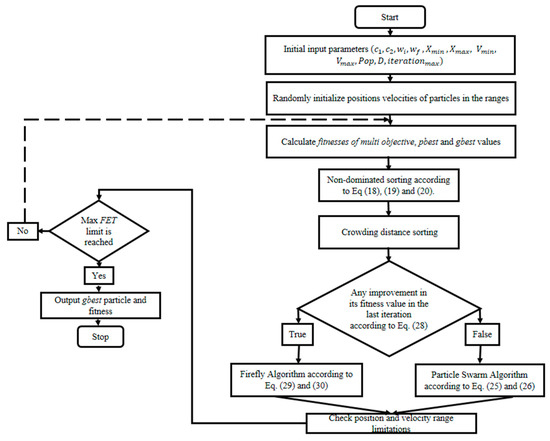
Figure 1.
Flowchart demonstrates the optimization procedure of the basic multi-objective hybrid firefly and particle swarm optimization (MOHFPSO) method.
Firstly, different input parameters are stated. Afterwards, initial positions and velocities of partials within their limits are initialized and global and local best particles are calculated according to Equations (18)–(20). After that, resulting fitness values are sorted based on non-dominated sorting, according to Equations (21) and (22), and compared in the last alteration. Finally, the current situation is kept and velocity vector and position are executed as following [34]:
where symbolizes fitness value of the particle and represents current position of particle, whereas denotes the previous global best value. r represents the specific distance and shows attraction.
FOA part will be executed if fitness value is same or improved as compared to the previous final best fitness value according to Equations (29) and (30). Else, the fitness value will be taken by the PSO part according to the Equations (25) and (26) for further improvement.
6. Application of the MOHFPSO Algorithm to Optimal Power Flow Problems
In this section, the proposed MOHFPSO algorithm was applied to OPF problems with a step by step procedure.
- Step 1.
- Describe the power system data that include real and reactive power limits, generators data, voltage limits of generator buses, initial values of active power, reactive power of capacitors and turn ratios of the tap-controlled transformers.
- Step 2.
- Simulate the basic power flow case and calculate the primary solutions of the particular objective functions, such as total generation cost, real power losses, voltage stability enhancement and voltage profile improvement, on the basis of Equations (1), (3), (4), and (6).
- Step 3.
- Define the general parameters, such as initial population (Pop), maximum iterations designed variables ) and its limits ), dimensions and algorithm specified parameters .
- Step 4.
- Locate positions of swarm population within a particular range as independent variables based on the following equations:where n and m denote the control and different solutions. Calculation of the j-th variable and k-th candidate solution is done as follows:k = 1, 2, 3, …, m, and j = 1, 2, 3, …, nwhere and are the limits of the j-th designed variables and denotes the random number within limits of (0–1). For more clarification, the physical components of can be formulated as follows:
- Step 5.
- Execute the load flow for every multi-objective function and compute the value of the specific objective function that relates to the solution.
- Step 6.
- Evaluate the fitness value for multi-objective and find the personal best (pbest) and global best (gbest) solutions according to Equations (18)–(20).
- Step 7.
- Sort the obtained fitness values based on non-dominated sorting according to Equations (21) and (22).
- Step 8.
- At this stage, crowding distance approach is applied.
- Step 9.
- Check the progress in the calculated values in the final iteration as stated by Equation (28).
- Step 10.
- Compute the result according to the modified vector of controlled variables. Calculate the new values of the objective functions and include the allocated penalty(ies) to the objective function if it violates the control variable limits, according to Equation (16).
- Step 11.
- Match the optimized value of objective function. If final values are optimized to earlier ones, then perform the Equations (29) and (30), otherwise apply the Equations (25) and (26) separately.
- Step 12.
- If termination criteria are met, then print the optimal solution values after stopping, else go back to stage 7.
For further explanation, flowchart of the proposed OPF problems based MOHFPSO algorithm is shown in Figure 2.
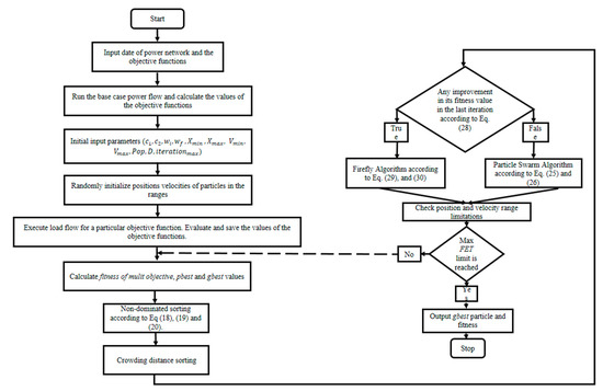
Figure 2.
The flowchart demonstrates the application of the MOHFPSO method for optimal power flow (OPF) problems.
7. Computational Results and Discussion
In this paper, MOHFPSO algorithm was used for optimization of total fuel cost (FC), optimization of real power loss (PL), optimization of voltage profile improvement or voltage deviations (VD) and optimization of voltage stability improvement (L-index). Five multi-objective functions with various combinations were taken to deal with the OPF problems. The program has been coded using MATLAB R2011a on a PC having 4 GHz Intel® Core™ i7 CPU with 8 GB RAM. The algorithm was executed 30 times. The achieved simulation results of the current work are discussed below. In order to show effectiveness of the proposed MOHFPSO algorithm, optimum values of the results were indicated with bolt face in corresponding tables. Standard IEEE 30-bus and 57-bus test [47] systems were applied to verify performance and effectiveness of the proposed algorithm.
The standard IEEE 30-bus test system comprises of six generator units installed at bus number 1, 2, 5, 8, 11 and 13. Loads are placed at 24 load buses. Four tap-controlled transformers are installed between branches 6–9, 6–10, 4–12 and 27–28 within the limits of 0.9–1.1. Turn ratios of the tap-controlled transformers, voltages of the generation units and reactive power injection, such as shunt capacitors, are taken as independent variables. The voltage magnitudes of generators and load buses are restricted within the limits of 0.95–1.05 p.u. and 0.9–1.05 p.u. Nine shunt-capacitors (VAr injectors), each having capacity of 5 MVAr and range of 0–30 MVAr, are placed at buses 10, 12, 15, 17, 20, 21, 23, 24 and 29. More detail of the IEEE 30-bus test system is mentioned in [47]. Firstly, the three bi-objective functions of OPF problems, such as FC and PL (Case-I), FC and VD (Case-II) and FC and L-index (Case-III) are optimized at the same time by applying MOHFPSO based method. In addition, two triple-objective functions of OPF problems, namely FC, PL and L-index (Case-IV) and FC, PL and VD (Case-V), are evaluated simultaneously by applying the proposed HFPSO method. Best results and optimal control variables of the above cases are mentioned in Table 1 (in bold) and Table A1, respectively. The obtained solutions of the MOHFPSO method for different cases are also compared with simulated results of the original PSO algorithm and various algorithms from current literature.

Table 1.
Optimum simulation results of Cases I–V for IEEE 30-bus power network “Multi-objective”.
7.1. Case I: Minimization of FC and PL
In this section, FC and PL are measured simultaneously as a first multi objective function in order to solve the OPF problems besides confirming its efficiency. Table 1 and Table A1 illustrate the acquired best results and optimum values of control variables of the proposed MOHFPSO technique (see Case I). Optimum results of the current case using the proposed method are compared with simulated results of original PSO and various methods mentioned in the current literature, such as NSGA-II [48], MJaya [49], QOMJaya [50], MOABC/D [51], MOTALBO [52] and MOMICA [53]. Detailed comparison of the optimum results is shown in Table 2 (with obtained values in Bold). Obtained values, considering FC and PL simultaneously as an objective function by applying the proposed HFPSO method, are 819.53 $/h and 5.6827 MW. However, minimum values of the original MOPSO method are 822.32 $/h and 5.7015 MW and require more CPU time per simulation (sec). It can be found that the proposed method achieved the best minimized values as compared to other techniques. Consequently, it is clear from Table 2 that the algorithmic efficiency of MOHFPSO concerns solution superiority. It is also clear from Figure 3 that the achieved Pareto optimal front of MOHFPSO algorithm is more optimized as compared to Pareto optimal front of original PSO algorithm.
Table 2.
Comparison studies for Case-I applying various bi-objective methods.
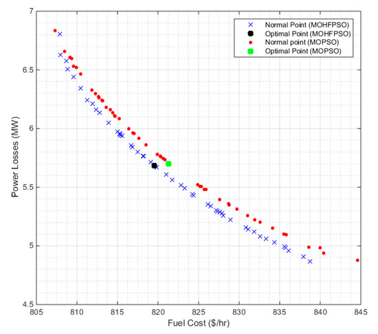
Figure 3.
The MOHFPSO and original PSO based Pareto optimal fronts for Case-I.
7.2. Case II: Minimization of FC and VD
In this part, FC and VD are calculated simultaneously as a second multi objective function to deal with the OPF problems as well as to check the effectiveness of the proposed MOHFPSO method. Table 1 explains the obtained best solutions and Table A1 shows the optimal control variables of the method (see Case II). Optimum solutions of this case from the proposed method are also compared with simulated results of original PSO and different techniques cited in the current literature work, such as BB-MPSO [54], MINSGA-II [54] and MOMICA [53]. Comparison of the optimum results in this case is presented in Table 3 (with optimum values in Bold). Achieved optimum solutions, in view of FC and VD simultaneously as a bi-objective function, by applying the proposed method are 803.2668 $/h and 0.1161 p.u. with less computational time per simulation (sec). On the other hand, the minimum values from the original MOPSO method are 803.694 $/h and 0.1122 p.u. Hence, it is concluded that the proposed MOHFPSO technique reached the best optimum solutions as compared to other methods. The achieved Pareto optimal front of proposed MOHFPSO method is compared to optimize the original MOPSO method, as plotted in Figure 4.
Table 3.
Comparison studies for Case-II applying various bi-objective methods.
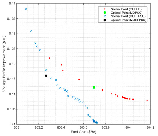
Figure 4.
The proposed MOHFPSO and original multi-objective particle swarm optimization (MOPSO) based Pareto optimal fronts for Case-II.
7.3. Case III: Minimization of FC and L-Index
In this section, FC and L-index or Lmax are simulated at the same time as a third multi objective function concerning the OPF problems in order to find usefulness of the proposed MOHFPSO technique. Table 1 describes the optimal solutions of the proposed MOHFPSO and original PSO methods (see Case III). Optimum values of the current case using the proposed technique are also matched with simulated values of original PSO and several methods taken from the present literature, such as NSGA-II [4], MOHS [4], MODE [55], MOTLBO [52], MOSPEA [56] and QOM-Jaya [50] separately. Broad comparison of the optimum solutions of this case and other algorithms is presented in Table 4 (with optimum solutions in Bold). Achieved optimum solutions, concerning FC and L-index simultaneously as a bi-objective function, by using the suggested MOHFPSO technique are 800.138 $/h and 0.1161 p.u. However, the minimum solutions of the original MOPSO method are 800.2531 $/h and 0.1122. It is, therefore, obvious from the comparison that the proposed technique reached the best minimum values as compared to those associated with other methods. It is evident from Table 4 that the algorithmic effectiveness of the proposed method is regarding solution dominance. The simulated Pareto optimal front of proposed MOHFPSO technique is better as compared to the original MOPSO technique, as graphed in Figure 5.
Table 4.
Comparison studies for Case-III applying various bi-objective methods.
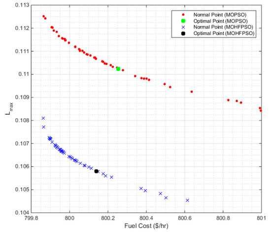
Figure 5.
The proposed MOHFPSO and original MOPSO based Pareto optimal fronts for Case-III.
7.4. Case IV: Minimization of FC, PL and L-Index
In this section, three objectives, such as FC, PL and L-index (i.e., max Lmax), were simulated simultaneously, as a fourth multi-objective function, using the proposed MOHFPSO and original PSO methods for OPF problems. Table 1 shows obtained optimum results for this case (see Case IV) and the optimal control variables of the case are represented in Table A1. Table 5 (with obtained optimum results in Bold) compares optimum solutions of this case by applying the proposed MOHFPSO method with original PSO and various methods from the current literature work, such as MJaya [50] and QOMJaya [50]. Obtained optimum results, as a triple-objective function, by using the recommended HFPSO method are 828.4980 $/h, 5.5700 MW and 0.1212. On the other hand, minimum values of the original MOPSO technique are 832.2023 $/h, 5.5024 MW and 0.1269. So, it is obvious from Table 5 that the proposed method achieves the best solutions as compared to other methods, in terms of its optimization efficacy. Furthermore, Figure 6 describes Pareto optimum fronts of FC, PL and L-index by applying proposed MOHFPSO and original MOPSO methods. It can be seen from the graphical representation in Figure 4 that the proposed method has finer Pareto front and improved solutions.
Table 5.
Comparison analysis for case-IV using different triple-objective methods.
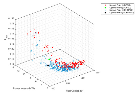
Figure 6.
Pareto fronts with MOHFPSO and MOPSO methods for Case-IV.
7.5. Case V: Minimization of FC, PL and VD
In this case, FC, PL and VD are simulated simultaneously, as a fifth triple-objective function for the OPF problems, by applying the proposed MOHFPSO technique. Optimum results of this case are presented in Table 1 (see Case-V). Comparison of optimum values of this case with original PSO technique is mentioned in Table 6 (with best obtained values in Bold). Moreover, best solution values of the proposed MOHFPSO method are 828.9908 $/h, 5.8563 MW, and 0.3392 p.u. However, best solution values of the original PSO technique are 830.6012 $/h, 5.8563 MW, and 0.3215 p.u. So, it is noticeable from the Table 6 that the proposed method obtained the best optimized values as compared to original methods. Furthermore, Figure 7 describes Pareto optimum fronts of FC, PL and VD by using the proposed MOHFPSO and original MOPSO methods. Graphical representation in Figure 5 shows that the proposed method has better Pareto optimal front.
Table 6.
Comparison analysis for Case-V using various triple-objective methods.
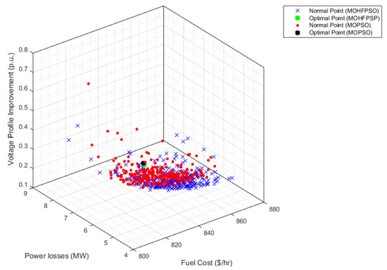
Figure 7.
Pareto fronts with proposed MOHFPSO and original MOPSO algorithms for Case-V.
A large scale, standard IEEE 57-bus test power system has been used to prove the robustness of the proposed method for OPF problems. The standard IEEE 57-bus test system includes seven generator units connected at bus number 1, 2, 3, 8, 6, 8, 9 and 12. Loads are installed at 42 load buses. 17 tap-controlled transformers are located at branches 19, 20, 31, 35, 36, 37, 41, 46, 54, 58, 59, 65, 66, 71, 73, 76 and 80 within the ranges of 0.9–1.1. Turn ratios of the tap-controlled transformers, voltages of the generation units and reactive power injection such as shunt capacitors are considered as independent variables. The voltage magnitudes of generators and load buses are restricted within the limits of 0.95–1.05 p.u. and 0.9–1.05 p.u. Three shunt-capacitors (VAr injectors), each having capacity of 5MVAr and range of 0–30 MVAr, are placed at buses 18, 25 and 53. More detail of the IEEE 57-bus test system is cited in [47]. Rest of the cases are tested based on IEEE 57-bus test system. Cases VI to VIII are bi-objective functions of OPF problems, such as FC and PL (Case-VI), FC and VD (Case-VII) and FC and L-index (Case-VIII) and optimized at the same time by using proposed MOHFPSO based method. In addition, Cases IX and X are triple-objective functions of OPF problems, namely FC, PL and L-index (Case-IX) and FC, PL and VD (Case-X) and are elevated simultaneously by applying the proposed method. Best results of the above all cases are mentioned in Table 7 (in Bold) and optimal values of control variables are represented in Table A2. The obtained solutions of the MOHFPSO method for various cases are also matched with simulated optimized results of the original MOPSO algorithm and various algorithms from present literature.
Table 7.
Optimum simulation results of Cases VI–X for IEEE 57-bus power network “Multi objective”.
7.6. Case VI: Minimization of FC and PL
In this case, two objectives functions, such as FC and PL, are simulated simultaneously, using the MOHFPSO and MOPSO techniques, as a bi-objective function for OPF problems. Control variables and optimum results of the current case are tabulated in Table A2 and Table 7 (see Case-VI) respectively. Furthermore, in Table 8 (with obtained results in Bold), the obtained optimum results are compared with the simulated values of PSO and different methods from literature, such as MOALO [57] and APFPA [58]. Best values of FC and PL, based on the proposed MOHFPSO technique, are 41,629.387 $/h and 12.4145 MW, as shown in Table 8. Figure 8 describes Pareto optimum fronts from the proposed MOHFPSO. It can be seen that the proposed method has finer Pareto front and improved solutions.
Table 8.
Comparison studies for Case-VI applying various bi-objective methods.
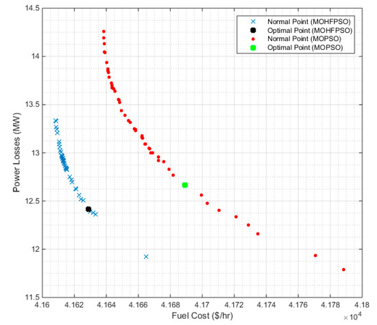
Figure 8.
The proposed MOHFPSO and original MOPSO based Pareto optimal fronts for Case-VI.
7.7. Case VII: Minimization of FC and VD
The current case shows the optimization of objectives functions, such as FC and DV simultaneously, as a seventh bi-objective function based on the proposed MOHFPSO method. Best solutions of the present case are shown in Table 7 (see Case-VII). Resulting minimum values from the proposed MOHFPSO, original MOPSO method and the literature, such as MODA [59], ECHT [60], PSO [61], SSO [61] and PSO-SSO [61] are compared in Table 9 (with obtained minimum values in Bold). Minimum values using the proposed method are 41,700.416 $/h and 0.8647 p.u., while the minimum values from the original MOPSO method are 41,782.65 $/h and 0.9592 p.u. Hence, Table 9 proves the capacity of the MOHFPSO over the PSO method based on optimization superiority. The proposed method also results in better Pareto optimal front as compared to the original PSO method, as shown in Figure 9.
Table 9.
Comparison studies for Case-VII applying various bi-objective methods.
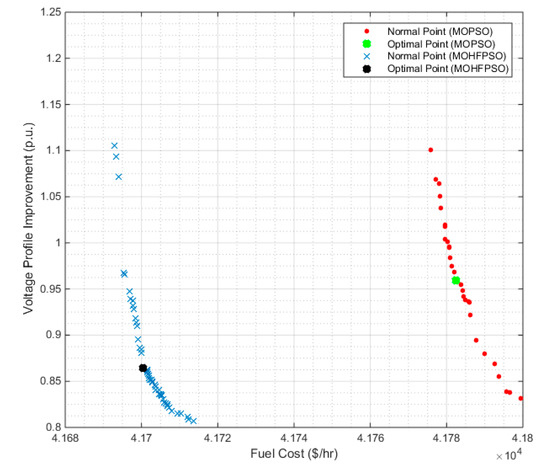
Figure 9.
The proposed MOHFPSO and original MOPSO based Pareto optimal fronts for Case-VII.
7.8. Case VIII: Minimization of FC, and L-Index
In this section, FC and L-index or Lmax are simulated as an eighth multi-objective function in order to solve the OPF problems based on the proposed MOHFPSO technique. Table A2 shows the optimal values of control variable of the proposed MOHFPSO and original MOPSO technique (see Case-VIII). Minimum values of the present case using the proposed technique are also matched with simulated values of original PSO in Table 10 (with obtained minimum values in Bold). Minimum values solving bi-objective function such as FC and L-index simultaneously of the proposed method are 41,601.043 $/h and 0.2001 p.u., and the minimum values of the original MOPSO technique are 41,606.46 $/h and 0.2018. Hence, the MOPSO method results in greater optimal values as compared to the proposed method, and Pareto optimal front of the original MOPSO technique is also worse as compared to the proposed MOHFPSO technique, as shown in Figure 10.
Table 10.
Comparison studies for Case-VIII applying various bi-objective methods.
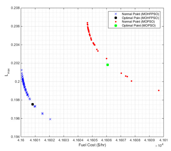
Figure 10.
The proposed MOHFPSO and original MOPSO based Pareto optimal fronts for Case-VIII.
7.9. Case IX: Minimization of FC, PL and L-Index
In this part, FC, PL and L-index (i.e., Lmax) have been taken as a ninth multi-objective, OPF function. Optimum values of control variable settings of the present case based on HFPSO are tabulated in Table A2 (see Case IX). Table 11 (with values in Bold) shows minimum value obtained from the proposed MOHFPSO algorithm, such as 41,726.379 $/h, 11.1026 MW and 0.2049 p.u., and the original PSO method, such as 41,836.5 $/h, 10.3812 MW and 0.2433 p.u. It is, therefore, evident that the proposed method achieves more optimized results as compared to the MOPSO method. Figure 11 shows Pareto optimum fronts using the proposed MOHFPSO and original MOPSO methods. It can be seen from the plot in Figure 9 that the proposed method has finer Pareto front.
Table 11.
Comparison analysis for Case-IX using various triple-objective methods.
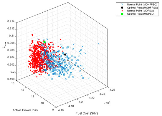
Figure 11.
Pareto fronts with the proposed MOHFPSO and original MOPSO methods for Case-IX.
7.10. Case X: Minimization of FC, PL and VD
In this section, FC, PL and VD are calculated simultaneously as a tenth multi-objective function for the OPF problems. Obtained results of the present case based on the proposed and MOPSO method are shown in Table 7 (see Case-X). Results are compared in Table 12 (with values in Bold to indicate the best results). Best solutions of the proposed method are 828.9908 $/h, 5.8563 MW and 0.3392 p.u., and best values of the original MOPSO technique are 830.6012 $/h, 5.8563 MW and 0.3215 p.u. Therefore, in the Table 12, it is evident that the proposed method achieves the best optimized values as compared to the original methods. Furthermore, Figure 12 describes Pareto optimum fronts of the current case.
Table 12.
Comparison study for Case-X using various triple-objective techniques.
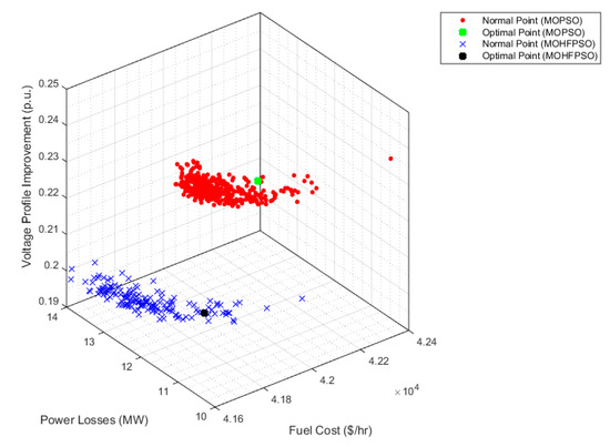
Figure 12.
Pareto fronts with proposed MOHFPSO and original MOPSO methods for Case-X.
8. Conclusions
In this paper, the basic purpose was to design and apply the MOHFPSO and MOPSO algorithms in order to solve the MOOPF problem based on non-dominated sorting and ideal distance minimization approach. In this research, three bi-objectives, which include simultaneous minimization of fuel cost and transmission loss, simultaneous minimization of fuel cost and voltage deviation and simultaneous minimization of fuel cost and L-index, and two tri-objective functions, which include simultaneous minimization of fuel cost with L-index and loss and simultaneous minimization of fuel cost with loss and voltage deviation were studied to authenticate the efficiency and capability of the MOHFPSO and MOPSO methods. The recommended algorithms were successfully tested on the IEEE 30-bus and IEEE 57-bus test networks to achieve optimal adjustment of the control variables to near global setting. The obtained simulated results of the proposed methods were compared with various optimization algorithms reported in the present literature. The comparison showed that the proposed MOHFPSO approach was more effective to achieve the best solution than MOPSO and the approaches in the current literature. It was also found that the MOHFPSO and MOPSO were potential means for treating multi-objective optimization problem, where several Pareto-optimal solutions could be found, in a single run, from the simulation results. However, the generated Pareto fronts were better and required short simulation time by applying MOHFPSO approach as compared to MOPSO method. Simulation time of the developed approach was high for a large scale system. Finally, it can be concluded that the above-mentioned MOHFPSO algorithm is motivating in consideration of simulation time for further work.
9. Future Work
The proposed techniques can be applied to more large-scale practical power systems based consideration of simulation time improvement to solve the other variants, such as optimal minimization of total emission and reactive power.
Author Contributions
A.K., H.H., N.I.A.-W. and M.L.O. developed the MOHFPSO algorithm for OPF problems. A.K. analyzed the data and algorithm, proved it and wrote the paper. H.H., N.I.A.-W. and M.L.O. contributed to ideas for the detailed discussion. A.K., H.H., N.I.A.-W. and M.L.O. reviewed the paper. All authors have read and agreed to the published version of the manuscript.
Funding
This research received no external funding.
Conflicts of Interest
The authors declare no conflicts of interest.
Appendix A
Table A1.
Optimum simulation control variables of Cases I–V for IEEE 30-bus power network “Multi-objective”.
Table A1.
Optimum simulation control variables of Cases I–V for IEEE 30-bus power network “Multi-objective”.
| Control Variable | Initial Status | Case I | Case II | Case III | Case IV | Case V | |||||
|---|---|---|---|---|---|---|---|---|---|---|---|
| MOHFPSO | MOPSO | MOHFPSO | MOPSO | MOHFPSO | MOPSO | MOHFPSO | MOPSO | MOHFPSO | MOPSO | ||
| PG1 (MW) | 99.248 | 132.9672 | 69.887 | 175.030 | 175.725 | 176.964 | 178.0319 | 137.08 | 71.093 | 140.773 | 119.1704 |
| PG2 (MW) | 80 | 50.8487 | 63.138 | 49.5777 | 49.3114 | 48.8429 | 49.2006 | 39.861 | 64.8319 | 41.4072 | 52.3021 |
| PG5 (MW) | 50 | 28.6418 | 50.000 | 21.7406 | 21.4884 | 21.3551 | 21.4066 | 37.067 | 48.2392 | 35.9052 | 33.7852 |
| PG8 (MW) | 20 | 35 | 35.000 | 22.6142 | 22.247 | 21.1517 | 21.8374 | 28.187 | 35 | 27.3027 | 31.198 |
| PG11 (MW) | 20 | 22.8993 | 30.000 | 12.2134 | 12.4712 | 11.9193 | 10 | 22.131 | 30 | 24.7157 | 30 |
| PG13 (MW) | 20 | 18.8816 | 38.443 | 12.0000 | 12 | 12 | 12 | 25.684 | 37.5742 | 20.2878 | 22.3005 |
| VG1 (p.u) | 1.05 | 1.1 | 1.1000 | 1.0421 | 1.0414 | 1.1 | 1.1 | 1.0478 | 1.1 | 1.1 | 1.0787 |
| VG2 (p.u) | 1.04 | 1.0892 | 1.0946 | 1.0251 | 1.024 | 1.1 | 1.1 | 1.0481 | 1.1 | 1.0649 | 1.0676 |
| VG5 (p.u) | 1.01 | 1.0643 | 1.0775 | 1.0142 | 1.014 | 1.0737 | 1.0734 | 1.0313 | 1.0824 | 1.0658 | 1.0421 |
| VG8 (p.u) | 1.01 | 1.0773 | 1.0869 | 1.0045 | 1.0053 | 1.0814 | 1.0819 | 1.0491 | 1.0881 | 1.0543 | 1.0507 |
| VG11 (p.u) | 1.05 | 1.1 | 1.1000 | 1.0466 | 1.0679 | 1.1 | 1.1 | 0.966 | 1.061 | 1.012 | 1.0542 |
| VG13 (p.u) | 1.05 | 1.0999 | 1.1000 | 0.9811 | 0.9856 | 1.1 | 1.1 | 1.053 | 1.0708 | 1.0421 | 1.0314 |
| T6,9 | 1.078 | 1.0423 | 1.0466 | 1.0688 | 1.0751 | 0.9976 | 0.9817 | 0.9405 | 0.9945 | 1.0216 | 1.0251 |
| T6,10 | 1.069 | 0.9 | 0.9000 | 0.9000 | 0.9 | 0.9 | 0.9 | 0.9948 | 0.9988 | 1.0353 | 1.0185 |
| T4,12 | 1.032 | 0.9941 | 0.9761 | 0.9379 | 0.9362 | 0.9499 | 0.9427 | 0.9755 | 1.0043 | 0.9154 | 1.0332 |
| T28,27 | 1.068 | 0.9785 | 0.9745 | 0.9705 | 0.9651 | 0.9205 | 0.9 | 0.9686 | 1.0083 | 0.9712 | 1.0015 |
| QC10 (Mvar) | 0 | 5 | 4.9546 | 2.7691 | 0.0057 | 5 | 5 | 1.5327 | 4.1368 | 1.5814 | 2.6662 |
| QC12 (Mvar) | 0 | 2.4017 | 4.4331 | 2.4519 | 0.7511 | 5 | 0 | 2.1635 | 3.0014 | 3.5097 | 2.7866 |
| QC15 (Mvar) | 0 | 4.1609 | 4.8996 | 4.9953 | 5 | 5 | 5 | 1.6641 | 3.1318 | 3.5327 | 2.6061 |
| QC17 (Mvar) | 0 | 3.3938 | 4.9325 | 5.0000 | 0.5524 | 5 | 0 | 2.4001 | 2.6075 | 2.8148 | 3.4346 |
| QC20 (Mvar) | 0 | 3.9695 | 5.0000 | 5.0000 | 5 | 5 | 5 | 4.753 | 1.0603 | 1.4796 | 1.7429 |
| QC21 (Mvar) | 0 | 0 | 5.0000 | 4.4838 | 5 | 5 | 5 | 4.213 | 1.601 | 1.3909 | 3.5982 |
| QC23 (Mvar) | 0 | 5 | 4.2653 | 4.9962 | 5 | 4.9999 | 5 | 3.383 | 4.6702 | 0.1871 | 2.0906 |
| QC24 (Mvar) | 0 | 0 | 5.0000 | 5.0000 | 5 | 5 | 5 | 4.1564 | 1.9945 | 3.0401 | 2.6266 |
| QC29 (Mvar) | 0 | 5 | 2.3369 | 2.6731 | 1.952 | 5 | 5 | 1.285 | 4.181 | 3.7882 | 1.7781 |
Table A2.
Optimum simulation control variables of Cases VI–X for IEEE 57-bus power network “Multi-objective”.
Table A2.
Optimum simulation control variables of Cases VI–X for IEEE 57-bus power network “Multi-objective”.
| Control Variable | Case VI | Case VII | Case VIII | Case IX | Case X | |||||
|---|---|---|---|---|---|---|---|---|---|---|
| MOHFPSO | MOPSO | MOHFPSO | MOPSO | MOHFPSO | MOPSO | MOHFPSO | MOPSO | MOHFPSO | PSO | |
| PG1 (MW) | 140.6333 | 155.1915 | 145.9066 | 123.75 | 141.3625 | 142.3974 | 137.9766 | 155.7437 | 154.0375 | 132.2372 |
| PG2 (MW) | 100 | 80.9419 | 89.558 | 75.466 | 100 | 87.7263 | 86.4643 | 65.4923 | 67.786 | 100 |
| PG3 (MW) | 40 | 44.7842 | 40 | 40 | 40 | 44.8455 | 40 | 45.3583 | 44.3832 | 57.6318 |
| PG6 (MW) | 68.3132 | 69.1368 | 73.7595 | 60.492 | 69.162 | 71.175 | 69.3992 | 63.9422 | 100 | 92.4105 |
| PG8 (MW) | 445.7546 | 435.2929 | 455.9187 | 473.44 | 458.6034 | 460.2767 | 469.2318 | 421.2054 | 387.1094 | 440.4937 |
| PG9 (MW) | 100 | 100 | 100 | 82.463 | 100 | 100 | 100 | 100 | 97.6074 | 30 |
| PG13 (MW) | 359.6073 | 377.0029 | 361.1385 | 410 | 355.7381 | 357.8237 | 361.4745 | 410 | 410 | 410 |
| VG1 (p.u) | 1.1 | 1.1 | 1.0313 | 1.0443 | 1.1 | 1.1 | 1.0965 | 1.1 | 1.1 | 1.1 |
| VG2 (p.u) | 1.1 | 1.1 | 1.0324 | 1.0558 | 1.1 | 1.1 | 1.0973 | 1.1 | 1.1 | 1.1 |
| VG3 (p.u) | 1.0917 | 1.0929 | 1.0178 | 1.0447 | 1.0924 | 1.0924 | 1.0893 | 1.1 | 1.1 | 1.0937 |
| VG6 (p.u) | 1.1 | 1.1 | 1.0406 | 1.0456 | 1.1 | 1.1 | 1.0895 | 1.1 | 1.1 | 1.1 |
| VG8 (p.u) | 1.1 | 1.1 | 1.0607 | 1.0706 | 1.1 | 1.1 | 1.1 | 1.1 | 1.1 | 1.1 |
| VG9 (p.u) | 1.1 | 1.0959 | 1.0388 | 1.0348 | 1.1 | 1.0959 | 1.0999 | 1.1 | 1.1 | 1.1 |
| VG13 (p.u) | 1.0864 | 1.0847 | 1.0245 | 1.037 | 1.0865 | 1.0861 | 1.0746 | 1.091 | 1.1 | 1.1 |
| QC18 (Mvar) | 20 | 6.3146 | 20 | 5.0984 | 20 | 20 | 2.5444 | 17.1254 | 10.3047 | 3.0548 |
| QC25 (Mvar) | 15.4808 | 14.1836 | 10.1919 | 14.236 | 11.9803 | 10.9924 | 15.2447 | 13.6022 | 15.6684 | 16.5082 |
| QC53 (Mvar) | 10.5882 | 10.0646 | 13.702 | 13.998 | 9.7685 | 0 | 7.3698 | 11.4095 | 8.2762 | 9.0105 |
| T4,18 | 0.9 | 1.0826 | 0.9591 | 0.9876 | 1.1 | 0.9 | 0.9 | 0.9 | 1.0226 | 0.9 |
| T4,18 | 1.1 | 0.9 | 1.1 | 1.0046 | 0.9 | 0.9 | 1.0094 | 1.0097 | 0.9014 | 0.9 |
| T21,20 | 1.0765 | 0.9231 | 1.1 | 0.9907 | 0.9 | 0.9 | 1.1 | 1.0464 | 1.0418 | 1.0184 |
| T24,25 | 1.0405 | 0.9459 | 0.9765 | 0.9815 | 0.9 | 0.9 | 0.9646 | 1.1 | 0.9186 | 1.0999 |
| T24,25 | 1.1 | 0.9275 | 1 | 1.0077 | 0.9347 | 0.9404 | 0.9431 | 1.0447 | 1.1 | 0.9016 |
| T24,26 | 0.9951 | 0.9 | 1.0179 | 1.0233 | 0.9612 | 0.9959 | 0.9913 | 0.9893 | 0.9967 | 1.008 |
| T7,29 | 0.9 | 0.9239 | 1.0081 | 1.0229 | 0.9 | 0.9 | 0.9 | 0.9 | 0.9 | 0.9 |
| T34,32 | 1.0123 | 0.9 | 0.9288 | 0.9451 | 0.9 | 0.9 | 0.9 | 1.1 | 0.9275 | 0.9 |
| T11,41 | 0.9 | 0.9 | 0.9 | 0.9 | 0.9 | 0.9363 | 0.932 | 0.9178 | 0.9437 | 0.9 |
| T15,45 | 0.9044 | 1.1 | 0.9713 | 0.9831 | 0.9344 | 0.9049 | 0.9 | 0.9 | 0.9 | 0.9 |
| T14,46 | 0.9 | 1.0457 | 0.9661 | 0.9809 | 0.93 | 0.9031 | 0.9 | 0.9023 | 0.9017 | 0.9 |
| T10,51 | 0.9107 | 1.0511 | 0.9844 | 0.9917 | 0.9267 | 0.9072 | 0.9 | 0.9 | 0.9107 | 0.9 |
| T13,49 | 0.9 | 1.0072 | 0.9433 | 0.9477 | 0.9113 | 0.9 | 0.9 | 0.9 | 0.9 | 0.9 |
| T11,43 | 0.9 | 1.0068 | 0.9645 | 0.9983 | 0.9 | 0.9117 | 0.9 | 1.1 | 0.9 | 1.1 |
| T40,56 | 1.1 | 0.9 | 1.0174 | 0.9735 | 0.9813 | 1.1 | 1.008 | 1.1 | 1.0188 | 1.1 |
| T39,57 | 0.9 | 0.9142 | 0.947 | 0.9697 | 0.9 | 1.0026 | 0.9 | 1.0836 | 1.0304 | 1.0794 |
| T9,55 | 0.9 | 0.9379 | 1.0198 | 1.0323 | 0.9 | 0.9 | 0.9 | 0.9 | 0.9 | 0.9 |
References
- Carpentier, J. Contribution à l’étude du Dispatching Economique. Bull. Soc. Fr. Electr. 1962, 8, 431–447. [Google Scholar]
- Carpentier, J. Optimal power flows. Int. J. Electr. Power Energy Syst. 1979, 1, 3–15. [Google Scholar] [CrossRef]
- Deb, K. Multi-Objective Optimization Using Evolutionary Algorithms: An Introduction. In Multi-Objective Evolutionary Optimisation for Product Design And Manufacturing; Wiley-Interscience Series in Systems and Optimization; Wiley-Interscience: New York, NY, USA, 2001. [Google Scholar]
- Sivasubramani, S.; Swarup, K.S. Multi-objective harmony search algorithm for optimal power flow problem. Int. J. Electr. Power Energy Syst. 2011, 33, 745–752. [Google Scholar] [CrossRef]
- Chen, Y.L. Weighted-norm Approach for Multiobjective VAr Planning; IET: London, UK, 1998. [Google Scholar] [CrossRef]
- Yalcinoz, T.; Köksoy, O. A multiobjective optimization method to environmental economic dispatch. Int. J. Electr. Power Energy Syst. 2007, 29, 42–50. [Google Scholar] [CrossRef]
- Dhillon, J.S.; Parti, S.C.; Kothari, D.P. Multiobjective optimal thermal power dispatch. Int. J. Electr. Power Energy Syst. 1994, 16, 383–389. [Google Scholar] [CrossRef]
- Chen, Y.L.; Liu, C.C. Multiobjective VAR planning using the goal-attainment method. IEE Proc. Gener. Transm. Distrib. 1994. [Google Scholar] [CrossRef]
- Ali Abou El-Ela, A.; El-Sehiemy, R.A.A.; Taha Mouwafi, M.; Salman, D.A.F. Multiobjective Fruit Fly Optimization Algorithm for OPF Solution in Power System. In Proceedings of the 20th International Middle East Power Systems Conference (MEPCON 2018), Cairo, Egypt, 18–20 December 2019. [Google Scholar] [CrossRef]
- Nguyen, T.T. A high performance social spider optimization algorithm for optimal power flow solution with single objective optimization. Energy 2019, 171, 218–240. [Google Scholar] [CrossRef]
- Bouchekara, H.R.E.H.; Chaib, A.E.; Abido, M.A.; El-Sehiemy, R.A. Optimal power flow using an Improved Colliding Bodies Optimization algorithm. Appl. Soft Comput. J. 2016, 42, 119–131. [Google Scholar] [CrossRef]
- Shafik, M.B.; Chen, H.; Rashed, G.I.; El-Sehiemy, R.A. Adaptive multi objective parallel seeker optimization algorithm for incorporating TCSC Devices into Optimal Power Flow Framework. IEEE Access 2019. [Google Scholar] [CrossRef]
- Zhang, J.; Wang, S.; Tang, Q.; Zhou, Y.; Zeng, T. An improved NSGA-III integrating adaptive elimination strategy to solution of many-objective optimal power flow problems. Energy 2019, 172, 945–957. [Google Scholar] [CrossRef]
- Attia, A.F.; El Sehiemy, R.A.; Hasanien, H.M. Optimal power flow solution in power systems using a novel Sine-Cosine algorithm. Int. J. Electr. Power Energy Syst. 2018, 99, 331–343. [Google Scholar] [CrossRef]
- El-Sattar, S.A.; Kamel, S.; El Sehiemy, R.A.; Jurado, F.; Yu, J. Single- and multi-objective optimal power flow frameworks using Jaya optimization technique. Neural Comput. Appl. 2019. [Google Scholar] [CrossRef]
- Elattar, E.E.; ElSayed, S.K. Modified JAYA algorithm for optimal power flow incorporating renewable energy sources considering the cost, emission, power loss and voltage profile improvement. Energy 2019, 178, 598–609. [Google Scholar] [CrossRef]
- Duman, S.; Güvenç, U.; Sönmez, Y.; Yörükeren, N. Optimal power flow using gravitational search algorithm. Energy Convers. Manag. 2012, 59, 86–95. [Google Scholar] [CrossRef]
- Niknam, T.; Narimani, M.r.; Jabbari, M.; Malekpour, A.R. A modified shuffle frog leaping algorithm for multi-objective optimal power flow. Energy 2011, 36, 6420–6432. [Google Scholar] [CrossRef]
- Rezaei Adaryani, M.; Karami, A. Artificial bee colony algorithm for solving multi-objective optimal power flow problem. Int. J. Electr. Power Energy Syst. 2013, 53, 219–230. [Google Scholar] [CrossRef]
- Bouchekara, H.R.E.H. Optimal power flow using black-hole-based optimization approach. Appl. Soft Comput. J. 2014, 24, 879–888. [Google Scholar] [CrossRef]
- Bouchekara, H.R.E.H.; Abido, M.A. Optimal power flow using differential search algorithm. Electr. Power Compon. Syst. 2014, 42, 1683–1699. [Google Scholar] [CrossRef]
- Mandal, B.; Kumar Roy, P. Multi-objective optimal power flow using quasi-oppositional teaching learning based optimization. Appl. Soft Comput. J. 2014, 21, 590–606. [Google Scholar] [CrossRef]
- Ghasemi, M.; Ghavidel, S.; Gitizadeh, M.; Akbari, E. An improved teaching-learning-based optimization algorithm using Lévy mutation strategy for non-smooth optimal power flow. Int. J. Electr. Power Energy Syst. 2015, 65, 375–384. [Google Scholar] [CrossRef]
- Roy, P.K.; Paul, C. Optimal power flow using krill herd algorithm. Int. Trans. Electr. Energy Syst. 2015, 25. [Google Scholar] [CrossRef]
- Elsakaan, A.A.; El-Sehiemy, R.A.; Kaddah, S.S.; Elsaid, M.I. An enhanced moth-flame optimizer for solving non-smooth economic dispatch problems with emissions. Energy 2018. [Google Scholar] [CrossRef]
- Shaheen, A.M.; Farrag, S.M.; El-Sehiemy, R.A. MOPF Solution Methodology. IET Gener. Transm. Distrib. 2017. [Google Scholar] [CrossRef]
- Bhowmik, A.R.; Chakraborty, A.K. Solution of optimal power flow using non dominated sorting multi objective opposition based gravitational search algorithm. Int. J. Electr. Power Energy Syst. 2015, 64, 1237–1250. [Google Scholar] [CrossRef]
- Ngo, T.T.; Sadollah, A.; Kim, J.H. A cooperative particle swarm optimizer with stochastic movements for computationally expensive numerical optimization problems. J. Comput. Sci. 2016, 13, 68–82. [Google Scholar] [CrossRef]
- Agarwal, P.; Mehta, S. Nature-Inspired Algorithms: State-of-Art, Problems and Prospects. Int. J. Comput. Appl. 2014. [Google Scholar] [CrossRef]
- Uymaz, S.A.; Tezel, G.; Yel, E. Artificial algae algorithm (AAA) for nonlinear global optimization. Appl. Soft Comput. J. 2015. [Google Scholar] [CrossRef]
- Wen, J.; Ma, H.; Zhang, X. Optimization of the occlusion strategy in visual tracking. Tsinghua Sci. Technol. 2016, 21, 221–230. [Google Scholar] [CrossRef]
- Tanweer, M.R.; Suresh, S.; Sundararajan, N. Self regulating particle swarm optimization algorithm. Inf. Sci. 2015, 294, 182–202. [Google Scholar] [CrossRef]
- Blum, C.; Belsa Aguilera, M.J.; Roli, A.; Sampels, M. Hybrid Metaheuristics—An Emerging Approach to Optimization; Springer: Berlin/Heidelberg, Germany, 2008; ISBN 978-3-540-78294-0. [Google Scholar] [CrossRef]
- Aydilek, İ.B. A hybrid firefly and particle swarm optimization algorithm for computationally expensive numerical problems. Appl. Soft Comput. J. 2018, 66, 232–249. [Google Scholar] [CrossRef]
- Thangaraj, R.; Pant, M.; Abraham, A.; Bouvry, P. Particle swarm optimization: Hybridization perspectives and experimental illustrations. Appl. Math. Comput. 2011, 217, 5208–5226. [Google Scholar] [CrossRef]
- Yang, X.S. Firefly algorithms for multimodal optimization. In Stochastic Algorithms: Foundations and Applications; Lecture Notes in Computer Science (Including Subseries Lecture Notes in Artificial Intelligence and Lecture Notes in Bioinformatics); Springer: Berlin/Heidelberg, Germany, 2009. [Google Scholar] [CrossRef]
- Fister, I.; Yang, X.S.; Brest, J. A comprehensive review of firefly algorithms. Swarm Evol. Comput. 2013, 13, 34–46. [Google Scholar] [CrossRef]
- Bhowmik, A.R.; Chakraborty, A.K. Solution of optimal power flow using nondominated sorting multi objective gravitational search algorithm. Int. J. Electr. Power Energy Syst. 2014, 62, 323–334. [Google Scholar] [CrossRef]
- Abou El Ela, A.A.; Abido, M.A.; Spea, S.R. Optimal power flow using differential evolution algorithm. Electr. Power Syst. Res. 2009, 91, 878–885. [Google Scholar] [CrossRef]
- Bouchekara, H.R.E.H.; Abido, M.A.; Boucherma, M. Optimal power flow using Teaching-Learning-Based Optimization technique. Electr. Power Syst. Res. 2014, 114, 49–59. [Google Scholar] [CrossRef]
- Nangia, U.; Jain, N.K.; Wadhwa, C.L. Multiobjective optimal load flow based on ideal distance minimization in 3D space. Int. J. Electr. Power Energy Syst. 2001, 23, 847–855. [Google Scholar] [CrossRef]
- Kennedy, J.; Eberhart, R. Particle Swarm Optimization. In Proceedings of the International Conference on Neural Networks (ICNN’95), Perth, Australia, 27 November–1 December 1995; Volume IV, pp. 1942–1948. [Google Scholar] [CrossRef]
- Yang, X.S. Firefly algorithm, Lévy flights and global optimization. In Research and Development in Intelligent Systems XXVI: Incorporating Applications and Innovations in Intelligent Systems XVII; Springer: London, UK, 2010. [Google Scholar] [CrossRef]
- Yang, X.-S. Firefly Algorithm, Stochastic Test Functions and Design Optimisation. Int. J. Bio-Inspired Comput. 2010, 2, 78–84. [Google Scholar] [CrossRef]
- Kora, P.; Rama Krishna, K.S. Hybrid firefly and Particle Swarm Optimization algorithm for the detection of Bundle Branch Block. Int. J. Cardiovasc. Acad. 2016. [Google Scholar] [CrossRef]
- Abd-Elazim, S.M.; Ali, E.S. A hybrid Particle Swarm Optimization and Bacterial Foraging for optimal Power System Stabilizers design. Int. J. Electr. Power Energy Syst. 2013. [Google Scholar] [CrossRef]
- Anonymous. Power Systems Test Case Archive; University of Washington: Washington, DC, USA, 2006. [Google Scholar]
- Jeyadevi, S.; Baskar, S.; Babulal, C.K.; Willjuice Iruthayarajan, M. Solving multiobjective optimal reactive power dispatch using modified NSGA-II. Int. J. Electr. Power Energy Syst. 2011. [Google Scholar] [CrossRef]
- Warid, W.; Hizam, H.; Mariun, N.; Abdul-Wahab, N.I. Optimal power flow using the Jaya algorithm. Energies 2016, 9, 678. [Google Scholar] [CrossRef]
- Warid, W.; Hizam, H.; Mariun, N.; Abdul Wahab, N.I. A novel quasi-oppositional modified Jaya algorithm for multi-objective optimal power flow solution. Appl. Soft Comput. J. 2018. [Google Scholar] [CrossRef]
- Medina, M.A.; Das, S.; Coello Coello, C.A.; Ramírez, J.M. Decomposition-based modern metaheuristic algorithms for multi-objective optimal power flow—A comparative study. Eng. Appl. Artif. Intell. 2014. [Google Scholar] [CrossRef]
- Nayak, M.R.; Nayak, C.K.; Rout, P.K. Application of Multi-Objective Teaching Learning based Optimization Algorithm to Optimal Power Flow Problem. Procedia Technol. 2012. [Google Scholar] [CrossRef]
- Ghasemi, M.; Ghavidel, S.; Ghanbarian, M.M.; Gharibzadeh, M.; Azizi Vahed, A. Multi-objective optimal power flow considering the cost, emission, voltage deviation and power losses using multi-objective modified imperialist competitive algorithm. Energy 2014. [Google Scholar] [CrossRef]
- Zeng, Y.; Sun, Y. Solving multiobjective optimal reactive power dispatch using improved multiobjective particle swarm optimization. In Proceedings of the The 26th Chinese Control and Decision Conference (2014 CCDC), Changsha, China, 31 May–2 June 2014. [Google Scholar]
- Varadarajan, M.; Swarup, K.S. Solving multi-objective optimal power flow using differential evolution. IET Gener. Transm. Distrib. 2008. [Google Scholar] [CrossRef]
- Kumari, M.S.; Maheswarapu, S. Enhanced Genetic Algorithm based computation technique for multi-objective Optimal Power Flow solution. Int. J. Electr. Power Energy Syst. 2010. [Google Scholar] [CrossRef]
- Herbadji, O.; Slimani, L.; Bouktir, T. Optimal power flow with four conflicting objective functions using multiobjective ant lion algorithm: A case study of the algerian electrical network. Iran. J. Electr. Electron. Eng. 2019. [Google Scholar] [CrossRef]
- Mahdad, B.; Srairi, K. Security constrained optimal power flow solution using new adaptive partitioning flower pollination algorithm. Appl. Soft Comput. J. 2016. [Google Scholar] [CrossRef]
- Herbadji, O.; Slimani, L.; Bouktir, T. Multi-objective optimal power flow considering the fuel cost, emission, voltage deviation and power losses using Multi-Objective Dragonfly algorithm. In Proceedings of the International Conference on Recent Advances in Electrical Systems, Hammamet, Tunisia, 22–24 December 2017; pp. 191–197. [Google Scholar]
- Biswas, P.P.; Suganthan, P.N.; Mallipeddi, R.; Amaratunga, G.A.J. Optimal power flow solutions using differential evolution algorithm integrated with effective constraint handling techniques. Eng. Appl. Artif. Intell. 2018. [Google Scholar] [CrossRef]
- Sehiemy, R.A.E.; Selim, F.; Bentouati, B.; Abido, M.A. A novel multi-objective hybrid particle swarm and salp optimization algorithm for technical-economicalenvironmental operation in power systems. Energy 2020, 193, 116817. [Google Scholar] [CrossRef]


© 2020 by the authors. Licensee MDPI, Basel, Switzerland. This article is an open access article distributed under the terms and conditions of the Creative Commons Attribution (CC BY) license (http://creativecommons.org/licenses/by/4.0/).