1. Introduction
The Off-Grid systems used nowadays are often referred to as Smart Grids, as they are based on intelligent data analysis, predictive models and optimizations in real time. They are yet another step in the development of a sustainable supply of electrical energy used for both industrial and household purposes. It is planned that in the future Smart Grids will integrate the activities of all participants of the energy market and will cover many processes: producing, transmitting, distributing, selling and managing energy by the end-users [
1]. It will surely be a complex energy solution which will enable effective steering of all elements of the power grid. Moreover, Smart Grid will also be an intelligent measurement system which will provide detailed information about all power grids in real time. The collected data will be sent to the control nodes administrating, managing and taking decisions, and everything will be supervised by intelligent information and predictive and decisive algorithms.
Currently used autonomous energy systems (Off-Grid systems) are already supplied by renewable sources (RES) and supported by energy storage. In such cases, various circumstances should be taken into consideration in comparison to standard systems of energy distribution and transmission. The stochastic and unstable character of the renewable energy sources results in low short-circuit power, which decreases the stability of parameters of the power quality (PQ) in the Off-Grid system [
2,
3]. The frequency (FREQ), voltage disturbance, total harmonic distortion of voltage (THDV) and current (THDC) and flicker severity are the most important power quality parameters [
4]).
It is then necessary to keep these parameters within required boundaries in order to provide reliable and safe performance of household appliances. These various circumstances have led many researchers to work on optimization tools that can detect and backwardly optimize the power quality parameters in order to fulfill the required limits in accordance with international standards. Relevant standards and methods of data analysis are presented in [
5,
6]. Algorithms based on machine learning [
7], known as Support Vector Machines (SVM) [
8,
9], Artificial Neural Networks (ANN) [
10,
11], Genetic Algorithms (GA) [
12] and their combinations, are the main approaches to this issue. On the other hand, there are scientific works in which methods, such as Wavelet Transformations (WT) [
13] or Fuzzy based detection [
14], are used for detecting the decrease of the power quality on the basis of learned patterns. Most research, as it results from [
5,
6], focuses on on-line executing and softening the effects of the power quality aggravation, but does not concentrate on predicting or avoiding such phenomena where they occur. While most available works consider predicting the total amount of energy production or consumption [
15], this paper focuses on the analysis of the influence of switching on devices in order to examine their influence on the power quality in a microgrid.
The ability to avoid a power quality disturbance was conceptually proposed and generally designed in an earlier study [
16], and this concept was entitled as Active Demand Side Management (ADSM). The following study proposed by Vantuch et al. headed towards the design and verification of the power quality forecasting module of the ADSM concept [
17]. The approximation of the power quality parameters future value is vital for the proper and timely reactions of ADSM, which brings the ability to avoid the predicted power quality disturbance by modifying the energy consumption (shifting load). According to our previous studies [
17,
18], power quality prediction represents a complex issue dependent on many variables. The stochastic natures of RES accompanied by randomly perturbed electric load patterns were successfully examined as the input variables for the power quality predictions. The question now arises—would it be valuable to use the decomposition on load patterns in order to use only its relevant parts? Or is the contribution of all appliances equal in the task of the power quality prediction?
Our goal is to find out which appliances have a negative impact on the power quality in the Off-Grid system. To test this, each time we combined three different appliances to create a total of 120 combinations. They were switched on and off in a defined interval. The response of the system, in the view of the power quality parameters, was measured and stored for statistical evaluations. They revealed the fact that the appliances were responsible for irregular power quality behavior, and which one of their features was the most relevant for this prediction. This study may be used to design deeper feature engineering procedures in the tasks of power quality parameters forecasting to increase their accuracy.
2. Methods
There are two fundamental international standards defining the power quality as a term. The first one is the European standard EN 50160, that is the main technical norm for the voltage quality in Europe. The second one is the series of technical norms and reports on electromagnetic compatibility EN 61000, which is very comprehensive and contains references concerning the limits, equipment and measurements for the voltage quality. Many parameters of the power quality are defined in EN 50160 and EN 61000. Although these standards complement each other, they also differ. One of the differences is that EN 50160 sets the limits for a higher number of harmonics; on the other hand, while not having any limits for as many harmonics as EN 50160, EN 61000 sets a limit for THDV [
19]. Voltage Variation (V), Frequency of the supply voltage (FREQ) and Harmonic voltage (THDV) are the power quality parameters necessary for the purpose of our study. Their defined limiting values are pointed out with regard to the standards mentioned in
Table 1.
To interpret the table, a short definition of voltage parameters used in the table follows. Firstly, Voltage Frequency is the fundamental frequency of the supply voltage. The harmonic voltage is a sinusoidal voltage with a frequency equal to an integer multiple of the fundamental frequency. Harmonic voltage is evaluated individually by its relative amplitude
Uh related to the fundamental Voltage
U1, where
h is the order of the harmonic. In general, the total harmonic distortion factor, (THDV), is calculated using the following equation:
The third parameter, the voltage magnitude variation, is defined as an increase or decrease of voltage caused by a variation of the total load of the distribution system. This requires defining two other terms. One of them is the supply voltage which is the RMS value at a given moment at a point of a common coupling measured over a given time interval. The second term, the nominal voltage of the system, is the voltage which designates the system and to which certain parameters are calculated, in our case voltage variations [
20,
21].
2.1. General Description of the Research Procedure
In order to carry out the research on the impact of household appliances on the quality of energy consumed by the end user, a series of laboratory tests and appropriate numerical calculations were previously performed. Preliminary studies using statistical methods have shown that there are several types of devices that have a large impact on changes in the power quality parameters. Therefore, it was decided to carry out a holistic analysis of the impact of home appliances on the power quality according to the procedure presented in
Figure 1.
The first stage of the presented procedure is laboratory measurement of individual appliances and their combinations (
Figure 1). Basic appliances that can be commonly used in a household were selected for the measurement, but the portfolio is further expanded and in case of finding interesting results, these will be published in a separate article. The main emphasis is on the division of devices due to the uninterrupted flow of electricity—some devices can be disconnected for the time needed for power supply, while some absolutely cannot be disconnected e.g., water heating, as it is always necessary to supply electricity for its proper functioning. For the resulting statistical evaluation, the voltage, current, phase and frequency on the AC (Alternating Current) side of the hybrid converter were measured, and the real and apparent power were determined from these values.
For repeatability of the measurements, the photovoltaic cells and other temporary energy sources were completely disconnected, and the source of energy was only a NiCd batteries bank. For the purpose of the experiment, batteries with a relatively large capacity (375 Ah) were used; however, for further experiments, the capacity will be reduced so that it better reflects the possibilities of purchasing energy storage for household needs. This type of battery was chosen mainly for its high resistance to discharge and longer life even during longer storage.
An interesting aspect was the measurement with fully charged batteries and at half the available energy (experimentally determined). The aim was to find out what effect the state of charge has on the operation of electrical appliances or on the failure-free operation of the DC/AC converter. The individual batteries were, therefore, separately charged to a maximum level of 1.35 V and experimental measurements were performed with SoC 100%. Furthermore, the batteries were discharged to about 1.2 V and test measurements were performed again at SoC 50%.
The measurements of electrical quantities in the system were provided by two National Instruments multifunction DAQ devices (
Figure 2). Such NI-USB 6216 [
22] were additionally equipped with the Elcom SCM-101 and Elcom SCM-111 devices that act as signal converters of electric voltage and AC current signals (
Table 2).
Then, the measurement devices sent the data via USB interface to the local computer on which the Off-Grid system application was running. The measurement of the energy quality in the Off-Grid system was provided by a KMB SMC 144 analyzer [
23]. The visualization of the control and the measurement data flow is shown in
Figure 2.
The next stage contains the data analysis, which is the basis of the study results. Such an analysis was performed in four steps which reflect the methods used in this application area. The first step is the Pearson and Kendall correlation analysis which is widely used to measure the degree of the relationship between linearly related variables. Further processing, conducted with the use of a method called t-distributed Stochastic Neighbor Settlement (t-SNE), allows the transformation of the resulting data into a space with a smaller number of dimensions, which is more suitable for implementing it in the control algorithms. The K-means algorithm is often used to determine a non-hierarchical cluster analysis.
It assumes that the clustered objects can be understood as points in some Euclidean space and that the number of clusters k is predetermined. Clusters are then defined by their centroids, which are points in the same space as the clustered objects. Objects are included in the cluster whose centroid is closest to them. The algorithm proceeds iteratively by starting from some (usually randomly selected) centroids, assigning points to them, recalculating the centroids so that it is the center of gravity of the cluster of points, then again assigning points to the newly determined centroids and so on, until the position of the centroid becomes stable. In this way, information about the main groups of appliances can be obtained, while the original correlation is specified using the Kraskov estimator, which estimates mutual information about a small data set with a nonlinear dependence structure.
The final objective is to achieve data that will lead to the implementation of a predictor that can be used in real household management in order to minimize a negative impact on the power quality. The obtained information has to be applied into the control algorithm of the system working under the Active Demand Side Management (ADSM) algorithm, which is based on the Demand Response (DR) principle.
The current development version of the Off-Grid system has fixed sockets assigned to the appliances. The consumption control system evaluates the appliance connection based on the socket ID and the pre-prepared measured waveforms of the appliances. Based on the evaluation of the ADSM algorithm, the control system starts the appliance or delays its start. During the evaluation, ADSM works with the prediction of electricity consumption and production. Based on this, the system predicts necessary energy resources for a given day.
2.2. Experiment Description
As mentioned above, ten selected appliances were combined into triplets resulting in 120 combinations. There are three connected appliances at once because single running appliances in a household are rather uncommon. In order to conduct measurements of the changes of the power quality parameters on a testing Off-Grid platform, the devices were always switched on for an identical period of time of 12 min. To avoid the stochastic and unstable character of a renewable power source and to keep short circuit power of the same value at all times, the system was supplied by charged batteries. Each combination of switched-on appliances was measured at two different States of Charge (SoC). A hybrid inverter was used to recharge the batteries after executing each experiment in order to achieve the same, defined, SoC. It should be mentioned that recharging the batteries of the testing system between experiments lasted 18 min. So, one cycle consisting of the load and recharge periods was 30 min long. Therefore, the measurement takes 60 h at one SoC. As we examined two SoCs, it is 120 h in total. The appliances were selected to represent all kinds of most common appliances in a household configuration (see
Table 3) and two battery levels were applied equally for all measurements (fully and half charged). These appliances were physically present during the tests, so nothing had to be substituted. The experiment did not use simulated appliances but real appliances, commonly available in the household goods stores.
The PQ parameter values were measured by a KMB SMC 144 device with an adjusted one-minute time scale. For each minute, the minimum, maximum and average values were stored and formed into a vector for further analysis. The frequency (FREQ), total harmonic distortion on voltage (THDV) and voltage (V) were the power quality parameters examined for the purpose of this paper.
2.3. Platform Description
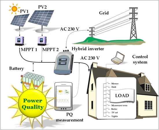
Figure 3 shows the Off-Grid system where two photovoltaic panels produce 2 kWp per each under normal conditions. However, for the reasons mentioned before, all the energy consumed by appliances was supplied from the batteries. A solar panel was not part of the experiment, nor the electricity grid, due to the same conditions for all tests (solar radiation intensity changes during the day). The Off-Grid system in this experiment was also equipped with a hybrid inverter, a battery bank, and a PQ measuring device. Conext XW + 8548 with the rated output power of 6.8 kW was used as the hybrid inverter. It also controlled the charging of the battery bank comprising of 40 Ferak 375 KPL batteries, where each NiCd battery had 375 Ah capacity and 1.2 V nominal voltage.
Table 4 gives a detailed information about the batteries.
The battery changes the voltage value during the discharge [
25]. When it is fully charged, each cell in the series produces approximately 1.5 V. At a 50% SoC, the cell voltage should be about 1.2 V and at the discharged state the voltage is close to 1 V. These values are applicable when the value of the discharge current is 0.1 C (nominal C-rate). Based on this, we performed an experiment at full and half SoC because the output on the alternating current side of the hybrid inverter could be affected by these parameters [
26]. The purpose was to eliminate the effect of the influence of the battery SoC on the power quality in a local Off-Grid system.
The appliances and the alternating current distribution grid were connected to the hybrid inverter via a switchboard controlled by control system software. This software controlled whether the defined appliance triplets were turned on in the defined schedule following the re-charging battery phase automatically. The measured data were also automatically stored in the system database for further analysis.
3. Testing and Analysis
The obtained measurements represented time series of continuous data where the switch-on phases were followed by the charging phases as it was set in our lab environment. The response of the power quality parameters to switching between those two phases is clearly visible in
Figure 4. One may assume a strong correlation between a higher load and a higher volatility of the PQ parameters, but this visible response of the power quality parameters is driven only by the changes between charging and discharging phases.
To prove this fact, we filtered the measured observations to examine only those where the load (S) was higher than 500 W. The estimation of correlation among load and power quality parameters on this filtered data will answer whether the volatility of the load parameter can reflect all power quality disturbances. Pearson [
27] and Kendall [
28] correlations were applied as correlation measures.
Figure 5 and
Figure 6 depict the pairwise relations between the power quality parameters responses to the varying load showing minimum or no correlation. This examination was performed on both scenarios having fully charged and half charged batteries.
Table 5 underlines these observations by computed correlations measures stating minimal or no progress similarity among the parameters. These results only reflect the true nature and difficulty of the problem, which is that the power quality response depends significantly not only on the current total load but on its varying character brought by one or several specific characters of an appliance. The following experiment is, therefore, designed to explore the dependencies between different combinations of appliances.
3.1. t-SNE Dimensionality Reduction
The proper normalization and dimensionality reduction were considered as necessary issues in order to set the common scale and omit redundancies and uncertainties in the obtained data. The t−SNE [
29] is a dimensionality reduction technique applied to process or visualize high-dimensional data. It converts similarities between data points
and
of a high dimensional space into a conditional probability
making use of
where
is the variance of the Gaussian centered on
. A perfect transformation will result into conditional probabilities
equal to
where
is a low-dimensional representation of
and their conditional probabilities are given by
The specific locations of the mapping points
should minimize the Kullback–Leibler divergence [
30,
31] of the distribution
from the distribution
which is performed making use of the gradient descent algorithm [
32] with respect to
.
It is highly recommended to use another dimensionality reduction method (e.g., principal component analysis [
33]) to reduce the number of dimensions to a lower level if the number of features is very high. This will suppress some noise [
34] and speed up the computation of the pairwise distances between samples. This approach has been successfully applied in many studies dealing with data mining or knowledge discovery tasks [
35,
36].
3.2. Gap Statistic Driven K-Means Clustering
The cluster analysis is a mechanism that labels the given samples according to their similarity or distance, which results in a clustering solution [
37]. Such process was found helpful in various applications [
38,
39], and, in our case, this process aims at extracting the groups of similar system responses to the power quality parameters. The clarity of a clustering solution with a minimum overlap can imply lower noisiness and uncertainty in data, while the inseparable highly overlapped clusters imply the presence of irrelevant data representation.
K-means clustering is an unsupervised machine learning approach that distinguishes the given samples
into an adjusted set of categories (clusters) in an iterative way. During each iteration, the observations are labelled
according to their closest centroid
(see Equation (5)). The centroids are further updated by averaging the positions of all members of their cluster (see Equation (6)). The first set of centroids are adjusted randomly and their number reflects the desired number of clusters. This converging process may be stopped after a fixed number of iterations or, simply, when the position alternation of a centroid is no longer required.
The number of clusters was determined by the gap statistic [
40]. It compares the total intra-cluster variation for different values of
k with their expected values under the data null reference distribution. The estimate of the optimal clusters will be a value that maximizes the gap statistic (i.e., one that yields the largest gap statistic). This means that the clustering structure is far from the random uniform distribution of points.
K-means fits into our work-flow due to its simplicity and interpretability. The motivation was not to produce state of the art relevancy estimation procedure, but rather to reveal that any work-flow built-up on reasonable, well described and widely applied algorithms could prove our findings. K-means is a typical representative of such building blocks.
3.3. Relevancy Estimation
The Kraskov algorithm is one of many approaches to estimate mutual information among two random variables. The Kraskov algorithm is widely used as it is considered as one of the most effective and accurate. It is able to evaluate the dependency among two multivariate variables in the same way as in the case of univariate variables. The Kraskov estimation is based on the Kozachenko–Leonenko entropy estimation [
41]:
where
N means the number of samples in
X,
d is the dimensionality of samples
x,
cd means the volume of a d-dimensional unitary ball and
is twice the distance (usually chosen as the Euclidean distance) from
xi to its
k-th neighbor. The most known derivate of the mutual information estimation has the following form (Equation (6)) [
41]:
where
is the number of points whose distance from
xi is not greater than
As we can see, the Kraskov’s mutual information does not require the computation of underlying probability distributions of the given variables, but it simply estimates the dependency by its neighbor-based clustering, which simplifies the entire approach.
4. Numerical Research Results
The examination procedure of power quality parameters was aligned as follows. The minimum, maximum and average values within a minute were measured for a 12-minute period, where the first and last minutes were skipped as transition events. The rest of the values were kept in a vector form. For each appliance configuration, we captured complete progress vectors. The values of the power quality parameter, in order to be clustered correctly, were normalized into a scale from 0 to 1. The t-SNE later performed the dimensionality reduction forming two-dimensional representations of the power quality data. They were clustered making use of a K-means clustering algorithm with an adjustable number of clusters decided by the applied gap statistic.
Within the separated groups, so called clusters, the average minimum, maximum, mean and standard deviations were computed to describe the nature of the power quality parameter progress defining a particular cluster. The probability of an appliance being a part of a configuration in a given cluster was computed to obtain additional information about which appliance may have the highest probability to perform a given progress of a power quality parameter.
To complete the appliance analysis on a deeper level, the appliance attributes were defined and their relevancy according to the given cluster was computed. This relevancy was estimated by mutual information estimation making use of the Kraskov algorithm. At this scale, the result will define which appliance attribute class possesses the highest nonlinear relation with the power quality parameter disturbance.
Each of the techniques mentioned above only pre-process the observed data or produce some partial results. The aim was to group the appliances behavior and on top of that identify which parameters are the most relevant for the found groups-as well as how significantly groups differ in the view of the power quality. This was demonstrated via the applied multi-step statistical analysis.
4.1. Fully Charged Battery
The first testing scenario was performed on the fully charged batteries. In total, 120 appliance combinations were separately switched on for 12-minute intervals and after each interval, the battery charging period followed. The batteries were charged to the full capacity in order to keep equal testing conditions for all examined appliance combinations.
The clustered behavior of appliance combinations with calculated probabilities of them being part of a given cluster is depicted in
Figure 7. As we can see, the visually clear separability was not obtained by all power quality parameters, the clusters are rather spread across the search space not forming separable entities. This may be caused by a varying impact of the appliances on the network or the network adjustment; therefore, the power quality responses are not significant enough.
However, some appliances, especially the microwave, the drill, the mower and the air conditioning heating, are able to be separated with a high accuracy, which means that their presence drives the system towards the specific behavior on a given power quality parameter. This behavior is defined by ranges of the power quality parameter values per cluster, which can be seen in
Table 6. A high probability of appliance being part of such a cluster may imply the causality that this specific appliance is a driver of a cluster specific power quality response. On the other hand, appliances with rather equal cluster membership probabilities may cause a minimal impact on the power quality behavior.
Specifically, FREQ values in the red cluster performed the highest standard deviation (as well as the highest min-max range), which is caused by the microwave due to its 100% probability of being in this cluster. This appliance possesses the highest load range, which may cause this power quality disturbance on a frequency parameter.
In the case of THDV, three appliances seem to possess a significant impact on the different behavior of this parameter. They are the drill, the microwave and the air conditioning heating having high probabilities forming the 2nd, the 3rd and the 4th cluster, respectively. The progress of the voltage parameter performed the visual separability of the lowest quality, but still, two appliances appeared to be significant for their kind of impact on this power quality parameter. The high probability of being part of the first cluster was gained by the mower, while the air conditioning heating obtained a comparable probability of being part of the second cluster.
Looking at the specific differences among the clusters, we can see the previously mentioned higher frequency standard deviation in the case of its second cluster, higher mean values of THDV in the cases of its second and third clusters and significant drops of power in the case of the first and second clusters of the V parameter.
Having the knowledge which appliance causes a specific behavior on the power quality parameter defined by a particular cluster, one may pose a question which parameter of the appliance may have the highest relevancy for this impact. The mutual information among the appliance features (see
Table 6) was estimated (see
Table 7). The electric load defining values possessed the highest relevancy towards the power quality parameter cluster labels followed by the switch type of the appliances. The resolution into inductive, capacitive or resistive characteristics for the appliance did not seem as relevant for the power quality disturbance.
4.2. Half Charged Battery
The second scenario performed similar metering steps, but the batteries were only half-charged for each appliance combination testing.
The appliance combinations clustered by their power quality parameters progress with estimated probabilities of their presence in the cluster are depicted in
Figure 8. The clearest separability was, as previously, achieved by the most sensitive parameter, the frequency. Similarly, the appliances with higher impact were the microwave, the air conditioning heating and the mower.
The statistical description of the modelled clusters performs differently, compared to the previous phase (see
Table 8 and
Table 9). In most cases, the ranges of minimum and maximum values were increased, with an increase of the standard deviation, which is caused by the lower short-circuit power of the system powered only by half-charged batteries.
The estimation of the relevancy among the appliance parameters and the cluster labels of power quality parameters revealed results comparable to the previous scenario, where the most relevant power factor of the appliance was its load and the switch type.
4.3. Example of Using the Achieved Research Results in a Real Off-Grid System
The managing of appliances in the Off-Grid system is provided by a control system built on the QUIDO input and output relay module [
42] with an Active Demand Side Management (ADSM) control algorithm based on the Demand Response (DR) principle. The Off-Grid system contains a number of common household appliances necessary for the simulation of a normal household. Appliances that are not physically connected in the system can be simulated by a controlled electronic load. The electronic load can be adjusted to a power of up to 4 kW with a step of 100 W and a power factor cos φ = 0.5, 0.95, 1. It is worth mentioning that the electronic load control program is a part of the developed LabVIEW application for controlling the hybrid Off-Grid system, which runs locally on a local computer placed directly in the Off-Grid system. The current state of application of the Off-Grid system is in the intermediate step before a complete migration from a local system control based on a PC to a cloud system.
To demonstrate the current version of the ADSM, the day when battery power is low in the morning has been chosen.
Table 10 shows the optimization of the operation of appliances carried out by the ADSM, so as not to discharge the batteries completely and thus shut down the Off-Grid system. This table is a demonstration and was made on the basis of the operation of a family home for a family of four. A change in the behavior of the control system for some items, where energy prediction would lead to the discharge of batteries, and are, therefore, decommissioned by the Off-Grid system or connected to the standard electrical network, can be read in the table. The laptop and microwave have a delayed supplying start while other appliances remain unchanged.
Figure 9 shows an example daily waveform of the total power consumption of appliances that would be powered by the batteries of the Off-Grid system before and after the ADSM intervention. The graph compares the operation of the Off-Grid system without optimization and with the ADSM optimization, where it can be seen that without its intervention there would be a complete discharge around 2 a.m. in the morning.
Figure 10 shows web-based user interfaces based on the QUIDO control system adapted for experimental measurement and visualization. The overview of all power sources and appliances is visualized in real-time in the system shown in
Figure 11. There are fundamental physical values such as electrical voltage, current, power etc. Moreover, state of devices and the energy flow direction in the Off-Grid system are presented.
Findings obtained by our study may significantly influence the future experiments related to the power quality predictive modeling. The quality of such models is heavily dependent on a set of relevant features, so called predictors, as it was identified in many studies presented in similar fields [
43,
44]. Those predictors are selected from the given dataset or aggregated making use of time shifts or statistical operations (floating mean, standard deviation, etc.). As our study revealed, the power quality is related to the kind of appliance that is executed at a given time. More specifically, based on the given appliance attributes, we may produce a categorical feature reflecting the current type of appliances operating in a system. Such feature will contribute to clarify whether a given load is likely to cause the power quality disturbance or not.
5. Conclusions
The research results presented in this article clearly show the negative influence of some devices on the microgrid power quality. For the purpose of the investigations, the most common household appliances were selected. Before the experiment, a market study of what appliances people normally have at home was conducted. It was proved that the influence of appliances on the power quality in the Off-Grid solar systems can be divided into clusters. Each cluster has a different level of influence on the parameters of the power quality in the Off-Grid system. Due to the conducted experiments, it is possible to focus on appliances having the greatest impact on the microgrid and to predict more precisely the disturbances of the power quality in this grid. It was also stated that each household appliance may be qualified to one of the determined clusters. Because each cluster has a specific influence on the power quality parameters in an Off-Grid, the control system can then optimize the schedule of switching on the appliances in order to avoid serious disturbances of the power quality.
The results of the experiments, presented in this paper, indicate that it was the microwave oven that affected the frequency parameter the most. As a result, a separate cluster, approved and visualized by a K-means algorithm and based on the Gap statistic, was created. Nevertheless, the frequency itself was stable and the standard deviation was not higher than 0.03.
The situation was similar for the THDV parameter, where the microwave oven, the air conditioning heating system and the drill were appliances that affected the system. The voltage was the last tested parameter. The experiments showed that its values were mainly affected by the lawn mower, the microwave oven and the air conditioning heating. In both cases, similar behaviors of the system were observed when the batteries were fully charged and half-charged of their nominal value. In the second mentioned case, the disturbances of the power quality were more significant, but their character and the source were of the same type.
The load value was determined as the most relevant feature of a device for the response to the power quality parameter. It was estimated with the use of Kraskov mutual information estimation, and then proved with probabilities of the most significant appliances generating the greatest loads and of the biggest standard deviations.
Summarizing the results of the research, it can be stated that the worked-out analysis may be applied to widen the functionality of the existing control systems in Off-Grids where the technology of the demand response is used. In such systems, control algorithms could also take into account the values of the power quality parameters before allowing particular appliances to start their function. Using such a functionality would significantly improve the power quality, especially in Off-Grid systems with high disturbances.
The subject of the present work seems interesting in terms of keeping satisfactory parameters of the power quality. In further work, it is planned to conduct other experiments, for example testing the connection and disconnection of the inverter to the electricity network and its effect on the operation of appliances and the quality of electricity, and data will be recorded in shorter time intervals in order to obtain more precise measurement values. Moreover, the enhancement of the number of appliances and combinations of their connections, as well as conducting a bigger number of experiments for various SoCs of batteries, will be the next element of our research. This will enable us to obtain additional data sets which will also contain the power quality disturbances of significantly greater values.
Author Contributions
V.B., M.P., Z.S. and S.M.; Methodology: V.B., M.P., Z.S. and T.V.; Software: T.V. and V.B.; Validation: Z.S., V.B., M.P. and W.W.; Visualization: T.V., W.W., Z.S.; Investigation: T.V., V.B., M.P. and Z.S.; Resources: V.B.; Data Curation: M.P.; Writing Original Draft Preparation: V.B., M.P., Z.S. and W.W.; Writing Review and Editing: Z.S. and W.W.; Supervision: S.M.; Project Administration: S.M. All authors have read and agreed to the published version of the manuscript.
Funding
This work has been supported by project TH02020191 High Density Modular Power Controllers for Automotive and Aerospace Systems, also by projects CZ.1.05/2.1.00/19.0389. Research Infrastructure Development of the CENET, SP2020/42. Development of algorithms and systems for control, measurement and safety applications VI and the research was carried out as part of the work WZ/WE-IA/2/2020 of the Bialystok University of Technology and financed from a subsidy provided by the Minister of Science and Higher Education.
Conflicts of Interest
The authors declare no conflict of interest.
References
- Vacheva, G.; Hinov, N.; Kanchev, H.; Stanev, R.; Cornea, O. Energy flows management of multiple electric vehicles in smart grid. Elektron. Elektrotechnika 2019, 25, 14–17. [Google Scholar] [CrossRef] [Green Version]
- Eckerbert, D.; Larsson-Edefors, P. Interconnect-driven short-circuit power modeling. In Proceedings of the Proceedings Euromicro Symposium on Digital Systems Design, Warsaw, Poland, 4–6 September 2001; pp. 414–421. [Google Scholar]
- Saradarzadeh, M.; Farhangi, S.; Schanen, J.L.; Jeannin, P.O.; Frey, D. Combination of power flow controller and short-circuit limiter in distribution electrical network using a cascaded h-bridge distribution-static synchronous series compensator. IET Gener. Transm. Distrib. 2012, 6, 1121–1131. [Google Scholar] [CrossRef]
- Broshi, A. Monitoring power quality beyond EN 50160 and IEC 61000-4-30. In Proceedings of the 9th International Conference on Electrical Power Quality and Utilisation, Barcelona, Spain, 9–11 October 2007. [Google Scholar]
- Saini, M.K.; Kapoor, R. Classification of power quality events—A review. Int. J. Electr. Power Energy Syst. 2012, 43, 11–19. [Google Scholar] [CrossRef]
- Mahela, O.P.; Shaik, A.G.; Gupta, N. A critical review of detection and classification of power quality events. Renew. Sustain. Energy Rev. 2015, 41, 495–505. [Google Scholar] [CrossRef]
- Stanelyte, D.; Radziukynas, V. Review of Voltage and Reactive Power Control Algorithms in Electrical Distribution Networks. Energies 2019, 13, 58. [Google Scholar] [CrossRef] [Green Version]
- Biswal, B.; Biswal, M.K.; Dash, P.K.; Mishra, S. Power quality event characterization using support vector machine and optimization using advanced immune algorithm. Neurocomputing 2013, 103, 75–86. [Google Scholar] [CrossRef]
- De Yong, D.; Bhowmik, S.; Magnago, F. An effective power quality classifier using wavelet transform and support vector machines. Expert Syst. Appl. 2015, 42, 6075–6081. [Google Scholar] [CrossRef]
- Valtierra-Rodriguez, M.; De Jesus Romero-Troncoso, R.; Osornio-Rios, R.A.; Garcia-Perez, A. Detection and classification of single and combined power quality disturbances using neural networks. IEEE Trans. Ind. Electron. 2014, 61, 2473–2482. [Google Scholar] [CrossRef]
- Raptis, T.E.; Vokas, G.A.; Langouranis, P.A.; Kaminaris, S.D. Total Power Quality Index for Electrical Networks Using Neural Networks. Energy Procedia 2015, 74, 1499–1507. [Google Scholar] [CrossRef] [Green Version]
- EL-Naggar, K.M.; AL-Hasawi, W.M. A genetic based algorithm for measurement of power system disturbances. Electr. Power Syst. Res. 2006, 76, 808–814. [Google Scholar] [CrossRef]
- Nath, S.; Dey, A.; Chakrabarti, A. Detection of power quality disturbances using wavelet transform. World Acad. Sci. Eng. Technol. 2009, 49, 869–873. [Google Scholar]
- Anis Ibrahim, W.R.; Morcos, M.M. An adaptive fuzzy self-learning technique for prediction of abnormal operation of electrical systems. IEEE Trans. Power Deliv. 2006, 21, 1770–1777. [Google Scholar] [CrossRef]
- Vantuch, T.; Vidal, A.G.; Ramallo-Gonzalez, A.P.; Skarmeta, A.F.; Misak, S. Machine learning based electric load forecasting for short and long-term period. In Proceedings of the IEEE World Forum on Internet of Things (WF-IoT 2018), Singapore, 5–8 February 2018; pp. 511–516. [Google Scholar]
- Misak, S.; Stuchly, J.; Vantuch, T.; Burianek, T.; Seidl, D.; Prokop, L. A holistic approach to power quality parameter optimization in AC coupling Off-Grid systems. Electr. Power Syst. Res. 2017, 147, 165–173. [Google Scholar] [CrossRef]
- Vantuch, T.; Misak, S.; Jezowicz, T.; Burianek, T.; Snasel, V. The Power Quality Forecasting Model for Off-Grid System Supported by Multiobjective Optimization. IEEE Trans. Ind. Electron. 2017, 64, 9507–9516. [Google Scholar] [CrossRef]
- Vantuch, T.; Stuchly, J.; Misak, S.; Burianek, T. Data mining application on complex dataset from the Off-Grid systems. Adv. Intell. Syst. Comput. 2015, 378, 63–75. [Google Scholar]
- Markiewicz, H.; Klajn, A. Voltage Disturbances Standard EN 50160—Voltage Characteristics in Public Distribution Systems. Wroc. Univ. Technol. 2004, 21, 215–224. [Google Scholar]
- British Standards Institution; DECC UK; Office for National Statistic; Met Office UK. Voltage characteristics of electricity supplied by public distribution systems. Whether Clim. Chang. 2010, 1, 1–18. [Google Scholar]
- European Std Committee EN 50160-2002. Voltage Characteristics of Electricity Supplied by Public Distribution Systems; European Std Committee EN 50160-2002: Brussels, Belgium, 2003. [Google Scholar]
- National Instruments USB-6216—NI. Available online: https://www.ni.com/pl-pl/support/model.usb-6216.html (accessed on 7 August 2020).
- K M B Systems s.r.o. SMC 144—KMB Systems. Available online: http://www.kmbsystems.cz/index.php/en/power-monitor-data-logger/smc-144 (accessed on 7 August 2020).
- Saft Ferak. Product Brochure: Ferak Ni-Cd Battery Range KPH-KPM-KPL-KPL LM; Saft Ferak: Pražmo, Czech Republic, 2020. [Google Scholar]
- Linden, D.; Reddy, T.B. Handbook of Batteries; McGraw-Hill: New York, NY, USA, 2002; ISBN 9780071359788. [Google Scholar]
- Ehnberg, J.; Liu, Y.; Grahn, M. Systems Perspectives on Renewable Power 2014; Sandén, B., Ed.; Chalmers: Göteborg, Sweden, 2015; p. 182. ISBN 9789198097405. [Google Scholar]
- Benesty, J.; Chen, J.; Huang, Y.; Cohen, I. Pearson correlation coefficient. Noise Reduct. Speech Process. 2009, 2, 1–4. [Google Scholar]
- Kendall, M.G. A New Measure of Rank Correlation. Biometrika 1938, 30, 81. [Google Scholar] [CrossRef]
- Van Der Maaten, L.; Hinton, G. Visualizing data using t-SNE. J. Mach. Learn. Res. 2008, 9, 2579–2625. [Google Scholar]
- Kullback, S.; Leibler, R.A. On Information and Sufficiency. Ann. Math. Stat. 1951, 22, 79–86. [Google Scholar] [CrossRef]
- Solomon, K. Letter to the Editor: The Kullback–Leibler distance. Am. Stat. 1987, 41, 340–341. [Google Scholar] [CrossRef]
- Ruder, S. An overview of gradient descent optimization algorithms. arXiv 2016, arXiv:1609.04747. [Google Scholar]
- Wold, S.; Esbensen, K.; Geladi, P. Principal component analysis. Chemom. Intell. Lab. Syst. 1987, 2, 37–52. [Google Scholar] [CrossRef]
- Li, W.; Cerise, J.E.; Yang, Y.; Han, H. Application of t-SNE to human genetic data. J. Bioinform. Comput. Biol. 2017, 15. [Google Scholar] [CrossRef]
- Vantuch, T.; Snasel, V.; Zelinka, I. Dimensionality Reduction Method’s Comparison Based on Statistical Dependencies. Procedia Comput. Sci. 2016, 83, 1025–1031. [Google Scholar] [CrossRef] [Green Version]
- Traven, G.; Matijevič, G.; Zwitter, T.; Žerjal, M.; Kos, J.; Asplund, M.; Bland-Hawthorn, J.; Casey, A.R.; De Silva, G.; Freeman, K.; et al. The Galah Survey: Classification and Diagnostics with t-SNE Reduction of Spectral Information. Astrophys. J. Suppl. Ser. 2017, 228, 24. [Google Scholar] [CrossRef]
- Kaufman, L.; Rousseeuw, P.J. Finding Groups in Data: An Introduction to Cluster Analysis; Wiley: Hoboken, NJ, USA, 1990; ISBN 9780471878766. [Google Scholar]
- Vantuch, T.; Fulneček, J.; Holuša, M.; Mišák, S.; Vaculík, J. An examination of thermal features’ relevance in the task of battery-fault detection. Appl. Sci. 2018, 8, 182. [Google Scholar] [CrossRef] [Green Version]
- Cecotti, H. Hierarchical κ-Nearest Neighbor with GPUs and a High Performance Cluster: Application to Handwritten Character Recognition. Int. J. Pattern Recognit. Artif. Intell. 2017, 31, 1750005. [Google Scholar] [CrossRef] [Green Version]
- Tibshirani, R.; Walther, G.; Hastie, T. Estimating the number of clusters in a data set via the gap statistic. J. R. Stat. Soc. Ser. B Stat. Methodol. 2001, 63, 411–423. [Google Scholar] [CrossRef]
- Kraskov, A.; Stögbauer, H.; Grassberger, P. Estimating mutual information. Phys. Rev. E Stat. Phys. Plasmas, Fluids Relat. Interdiscip. Top. 2004, 69, 16. [Google Scholar] [CrossRef] [Green Version]
- Papouch I/O modules | Papouch.com. Available online: https://en.papouch.com/io-modules/ (accessed on 7 August 2020).
- Zor, K.; Timur, O.; Teke, A. A state-of-the-art review of artificial intelligence techniques for short-term electric load forecasting. In Proceedings of the 2017 6th International Youth Conference on Energy (IYCE), Budapest, Hungary, 21–24 June 2017; pp. 1–7. [Google Scholar]
- Ghadimi, N.; Akbarimajd, A.; Shayeghi, H.; Abedinia, O. Two stage forecast engine with feature selection technique and improved meta-heuristic algorithm for electricity load forecasting. Energy 2018, 161, 130–142. [Google Scholar] [CrossRef]
Figure 1.
Diagram showing the scope of research presented in this article.
Figure 1.
Diagram showing the scope of research presented in this article.
Figure 2.
The Off-Grid measurement and the control system data flow.
Figure 2.
The Off-Grid measurement and the control system data flow.
Figure 3.
Scheme of the tested platform.
Figure 3.
Scheme of the tested platform.
Figure 4.
Sample of PQ parameters time plot shows the load and charging phase.
Figure 4.
Sample of PQ parameters time plot shows the load and charging phase.
Figure 5.
Pairwise relations among PQ parameters and the related load on a 100% SoC battery for: (a) voltage total harmonic distortion, (b) frequency, (c) voltage.
Figure 5.
Pairwise relations among PQ parameters and the related load on a 100% SoC battery for: (a) voltage total harmonic distortion, (b) frequency, (c) voltage.
Figure 6.
Pairwise relations among PQ parameters and the related load on a 50% SoC battery setup for: (a) voltage total harmonic distortion, (b) frequency, (c) voltage.
Figure 6.
Pairwise relations among PQ parameters and the related load on a 50% SoC battery setup for: (a) voltage total harmonic distortion, (b) frequency, (c) voltage.
Figure 7.
Clustering solutions of PQ parameters progresses at SoC 100% with the calculated probabilities of appliances being part of the particular cluster: (a,d)—voltage frequency (FREQ) with appliance probabilities, (b,e)—total harmonic distortion of voltage (THDV) with appliance probabilities and (c,f)—V with appliance probabilities.
Figure 8.
Clustering solutions of PQ parameters progress on SoC 50% with the calculated probabilities of appliances being part of the particular cluster: (a,d)—FREQ with appliance probabilities, (b,e)—THDV with appliance probabilities and (c,f)— voltage (V) with appliance probabilities.
Figure 8.
Clustering solutions of PQ parameters progress on SoC 50% with the calculated probabilities of appliances being part of the particular cluster: (a,d)—FREQ with appliance probabilities, (b,e)—THDV with appliance probabilities and (c,f)— voltage (V) with appliance probabilities.
Figure 9.
The comparison of non-optimized and optimized energy components in an Off-Grid system.
Figure 9.
The comparison of non-optimized and optimized energy components in an Off-Grid system.
Figure 10.
The web page generated by the control system, visualizing home appliances actual states.
Figure 10.
The web page generated by the control system, visualizing home appliances actual states.
Figure 11.
Smart Grid Laboratory (SGL) on-line visualization of the used appliances and the power sources.
Figure 11.
Smart Grid Laboratory (SGL) on-line visualization of the used appliances and the power sources.
Table 1.
Values of International Standards for power quality (PQ) [
20,
21].
Table 1.
Values of International Standards for power quality (PQ) [
20,
21].
| Parameter | EN 50160 | EN 61000 |
|---|
| Voltage frequency | Mean value measured over 10 s
±1% (49.5 Hz ÷ 50.5 Hz) for 99.5%
of week
−6%/+4% (47 ÷ 52 Hz) for 100% of week | ±2% |
| Voltage magnitude variations | Mean 10 min RMS values
±10% for 95% of week | ±10% applied for 15 min |
| Harmonic Voltage (% of fundamental supply voltage) | 5% 3rd, 6% 5th, 5% 7th, 1.5% 9th, 3.5 % 11th 3% 13th, 0.5% 15th 2% 17th, 1.5% 19th 23rd and 25th | 6% 5th, 5% 7th, 3.5% 11th, 3% 13th, THD < 8% |
Table 2.
Elcom SCM-101 and SCM-111 products parameters.
Table 2.
Elcom SCM-101 and SCM-111 products parameters.
| Device Name | Device Range | Input Value | Transfer Constant | Typical Input Resistance | Limiting
Error Value | Overload Capacity t < 1 s |
|---|
| SCM-101 | 600 V | ±600V | 100 V/1 V | 90 kΩ | 0.25% | 1000 V AC |
| 300 V | ±300 V | 50 V/1 V | 45 kΩ | 0.25% | 500 V AC |
| SCM-111 | 25 A | ±25 A | 4 A/1 V | <3 mΩ | 0.25% | 36 A |
| 12 A | ±12 A | 2 A/1 V | <6 mΩ | 0.25% | 18 A |
Table 3.
The properties of the appliances for their relevancy estimation.
Table 3.
The properties of the appliances for their relevancy estimation.
| Appliance | Load (W) | Power Factor (-) | Power Supply 1 |
|---|
| Avg | Min | Max | Value | Type | Type |
|---|
| Mower | 537.6 | 532.1 | 549.27 | 0.52 | Inductive | Continuous |
| Drill | 157.1 | 149.5 | 167 | 0.49 | Inductive | Continuous |
| Kettle | 919.1 | 917 | 928.3 | 1 | Resistive | Continuous |
| Fridge | 207.6 | 195.5 | 219.5 | 0.72 | Inductive | Continuous |
| Switched power supply | 410 | 409.7 | 420.2 | 0.78 | Capacitive | Switched |
| Air conditioner (AC) heating | 880 | 852.5 | 910 | 0.91 | Inductive | Continuous |
| Microwave oven | 203 | 76.8 | 1348.3 | 0.84 | Inductive | Switched |
| Boiler | 307 | 305.8 | 346.5 | 0.99 | Resistive | Continuous |
| TV set | 44 | 42.8 | 50.5 | 0.6 | Capacitive | Switched |
| Lights (CFL, LED) | 156 | 152.5 | 165.1 | 0.84 | Capacitive | Switched |
Table 4.
Features of the Ferak KPL 375 NiCd batteries [
24].
Table 4.
Features of the Ferak KPL 375 NiCd batteries [
24].
| Parameters | Value |
|---|
| Nominal Voltage (V) | 1.2 |
| Rated capacity (Ah) | 375.0 |
| Nominal C-rate (-) | 0.1 |
| Max C-rate (-) | 2.0 |
Table 5.
Correlations coefficients between PQ parameters and load parameter.
Table 5.
Correlations coefficients between PQ parameters and load parameter.
| Correlation | SoC (%) | THDV | FREQ | V |
|---|
| Pearson | 100 | −0.396 | 0.001 | −0.154 |
| 50 | −0.563 | 0.043 | −0.354 |
| Kendall | 100 | −0.285 | −0.116 | −0.154 |
| 50 | −0.388 | −0.131 | −0.173 |
Table 6.
Statistical description of the PQ parameters of the obtained clusters at SoC 100%.
Table 6.
Statistical description of the PQ parameters of the obtained clusters at SoC 100%.
| PQ Parameter | Cluster | Avg Min | Avg Max | Avg std | Avg Mean |
|---|
| FREQ (Hz) | 1st | 50.00 | 50.06 | 0.01 | 50.01 |
| 2nd | 49.97 | 50.07 | 0.03 | 50.01 |
| 3rd | 49.99 | 50.02 | 0.01 | 50.01 |
| THDV (%) | 1st | 1.20 | 6.91 | 0.76 | 3.66 |
| 2nd | 1.15 | 7.44 | 1.49 | 4.35 |
| 3rd | 1.27 | 7.26 | 0.85 | 5.04 |
| 4th | 1.19 | 7.74 | 1.24 | 3.30 |
| V (V) | 1st | 203.83 | 241.56 | 4.99 | 224.63 |
| 2nd | 208.28 | 242.27 | 5.24 | 225.53 |
| 3rd | 216.95 | 240.79 | 3.39 | 227.85 |
Table 7.
Mutual information estimated among the appliance features and cluster labels derived from the PQ parameters measured at SoC 100%.
Table 7.
Mutual information estimated among the appliance features and cluster labels derived from the PQ parameters measured at SoC 100%.
| | Loads | Power Factor | Switch Type |
|---|
| FREQ | 0.46 | 0.06 | 0.42 |
| THDV | 0.35 | 0.09 | 0.25 |
| V | 0.33 | 0.1 | 0.03 |
Table 8.
Statistical description of the PQ parameters of the obtained clusters for system 50% SoC.
Table 8.
Statistical description of the PQ parameters of the obtained clusters for system 50% SoC.
| PQ Parameter | Cluster | Avg Min | Avg Max | Avg std | Avg Mean |
|---|
| FREQ (Hz) | 1st | 49.99 | 50.09 | 0.02 | 50.01 |
| 2nd | 49.97 | 50.07 | 0.03 | 50.01 |
| 3rd | 49.98 | 50.03 | 0.01 | 50.01 |
| THDV (%) | 1st | 1.24 | 7.88 | 0.95 | 5.40 |
| 2nd | 1.24 | 7.88 | 1.27 | 3.24 |
| 3rd | 1.14 | 7.96 | 1.52 | 4.30 |
| 4th | 1.17 | 6.74 | 0.72 | 3.70 |
| V (V) | 1st | 198.51 | 241.53 | 5.67 | 224.80 |
| 2nd | 218.29 | 240.34 | 3.34 | 227.65 |
| 3rd | 209.66 | 241.86 | 4.98 | 225.56 |
Table 9.
Mutual information estimated among the appliance features and cluster labels derived from PQ parameters measured at SoC 50%.
Table 9.
Mutual information estimated among the appliance features and cluster labels derived from PQ parameters measured at SoC 50%.
| | Loads | Power Factor | Switch Type |
|---|
| FREQ | 0.38 | 0.02 | 0.32 |
| THDV | 0.31 | 0.06 | 0.28 |
| V | 0.34 | 0.01 | 0.04 |
Table 10.
The example appliance plan after the Active Demand Side Management (ADSM) optimization achieved in the experiment.
Table 10.
The example appliance plan after the Active Demand Side Management (ADSM) optimization achieved in the experiment.
| Appliance | Start | Stop | Start | Stop | System Schedule Change |
|---|
| Fridge | 00:00 | 00:00 | - | - | Unchanged |
| Air conditioning | 00:00 | 00:00 | - | - | Unchanged |
| Washing machine | 07:00 | 09:00 | - | - | Excluded from the plan,
the appliance will be powered from the grid |
| Kettle | 08:00 | 08:05 | - | - | Unchanged |
| TV set | 09:00 | 11:00 | - | - | Unchanged |
| Boiler | 00:00 | 08:00 | - | - | Excluded from the plan,
the appliance will be powered from the grid |
| Personal computer | 05:00 | 10:00 | - | - | Excluded from the plan,
the appliance will be powered from the grid |
| Notebook | 05:00 | 10:00 | 10:15 | 17:30 | Start delayed |
| Microwave oven | 06:00 | 06:05 | 11:25 | 11:30 | Start delayed |
| Boiler | 20:00 | 21:00 | - | - | Excluded from the plan,
the appliance will be powered from the grid |
| TV set | 07:00 | 09:00 | - | - | Unchanged |
| Lights | 07:00 | 09:00 | - | - | Unchanged |
| Kettle | 17:00 | 17:05 | - | - | Unchanged |
| Lights | 17:00 | 23:00 | - | - | Unchanged |
| Kettle | 09:00 | 09:05 | - | - | Unchanged |
© 2020 by the authors. Licensee MDPI, Basel, Switzerland. This article is an open access article distributed under the terms and conditions of the Creative Commons Attribution (CC BY) license (http://creativecommons.org/licenses/by/4.0/).

 ,
, 


