AE-LSTM Based Deep Learning Model for Degradation Rate Influenced Energy Estimation of a PV System

Abstract

With the increase in penetration of photovoltaics (PV) into the power system, the correct prediction of return on investment requires accurate prediction of decrease in power output over time. Degradation rates and corresponding degraded energy estimation must be known in order to predict power delivery accurately. Solar radiation plays a key role in long-term solar energy predictions. A combination of auto-encoder and long short-term memory (AE-LSTM) based deep learning approach is adopted for long-term solar radiation forecasting. First, the auto-encoder (AE) is trained for the feature extraction, and then fine-tuning with long short-term memory (LSTM) is done to get the final prediction. The input data consist of clear sky global horizontal irradiance (GHI) and historical solar radiation. After forecasting the solar radiation for three years, the corresponding degradation rate (DR) influenced energy potentials of an a-Si PV system is estimated. The estimated energy is useful economically for planning and installation of energy systems like microgrids, etc. The method of solar radiation forecasting and DR influenced energy estimation is compared with the traditional methods to show the efficiency of the proposed method.

1. Introduction

Forecasting correct power energy over a span of time is essential for the growth of, and getting benefits from, photovoltaic (PV) technology. Most important factors are the efficiency with which sunlight is converted into power and how this relationship changes with passing time. The degradation rate (DR) is a useful parameter to understand the power decline over a span of time, which plays a key role for PV technology beneficiaries like power companies, businesses and researchers, etc. DR is important from the economical point of view, as higher DR results in decreased power generation over time, consequently decreasing future cash flow [1]. Inaccurate calculation of degradation rates results in increased financial risk [2]. Degradation mechanisms are also important from a technical point of view, as they lead to failure of the system [3]. Therefore, finding out the science of degradation through modeling and experiments will lead to lifetime improvements.

Due to the low costs of production and having smaller coefficients of temperature, thin-film modules are becoming more popular day by day in the solar power market [4,5]. However, due to their susceptibility to changes in temperature and spectrums, the efficiency of these thin modules degrades with the passage of time. Mostly, research is being carried out for power delivery prediction using statistical and physical methods without any consideration of the DR impact [6,7,8,9]. Only limited studies are carried out on energy estimation considering the influence of degradation rates [10,11]. Solar radiation is the key parameter in solar generation and DR influenced energy estimation. Using only historical solar radiation as input, the paper [10] adopted different machine learning methods to predict solar radiation for three years ahead, and then derived the conclusion that random forest regression (RFR) brought out the most accurate estimation. However, the said paper lacks a clear explanation about the method of data management and processing for long-term prediction, which is very important.

The nature of the solar radiation forecasting problem is the time series. In time series problems, next time step output is dependent on past time step outputs. Deep learning has shown great success in dealing with time series problems [12,13,14]. Specifically, extensions of recurrent neural network, i.e., long short-term memory unit (LSTM) and gated recurrent unit (GRU) are more suitable for time series problems, due to their inherent characteristics of learning long-term dependencies [15,16]. Mostly, deep learning model-based forecasting is short-term forecasting ranging from a few hours to days [17,18,19]. Multi-time steps ahead solar irradiance forecasting of up to 120 minutes is performed in [20]. However, DR influenced energy estimation requires solar radiation data over a longer span of time. Year ahead solar radiation was forecasted using simple LSTM and GRU models [17]. However, these methods were trained in a supervised manner without optimal feature extraction and did not estimate the DR influenced energy of PV systems.

Auto-encoders (AEs) are effective in unsupervised feature extraction and dimensionality reduction [21,22]. In AE, the model is trained to reconstruct the input using a backpropagation algorithm [23]. AE first encodes the input into low dimensionality representations, and then reconstructs the input through the decoding process. In this paper, a combination of AE and LSTM, i.e., an AE-LSTM model is proposed for long-term solar radiation forecasting and PV energy estimation, in order to utilize the feature extraction ability of AE and the long-term dependency learning ability of LSTM. Firstly, features are extracted by training an AE model with input data. Then fine-tuning of the trained encoder part of the AE with the LSTM model is done to forecast solar radiation for the year ahead. Therefore, the main contributions of this paper are an AE-LSTM based deep learning model for three years ahead solar radiation forecasting and then corresponding DR influenced energy estimation of the PV system. Historical solar radiation data as well as clear sky global horizontal irradiance (GHI) are used as input data. The paper is divided into six sections: Section 2 contains methodology, which includes data selection and management. Section 3 explains the proposed AE-LSTM deep learning model. Section 4 gives the experiments and results. A comprehensive discussion is made in Section 5. Section 6 is the conclusion.

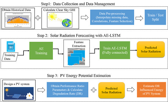
2. Methodology

Figure 1 shows the overall methodology. It can be seen from this figure that the proposed methodology is divided into three steps. The first step consists of data gathering and preprocessing. The preprocessing includes filling in of missing data by interpolation techniques [24], selection of appropriate input features by finding correlations and splitting the data into training and testing sets. The second step consists of the proposed deep learning model for solar radiation forecasting. In this step, first the AE model is trained to extract the underlying features in the input data. The extracted AE features are combined with LSTM layers to form a fully connected predictive model (AE-LSTM). In the final step, a PV system is designed in the horizon of forecasted solar radiation. Using appropriate parameters along with the forecasted radiation, DR influenced energy of the designed PV system is estimated for three years ahead. The following subsections explain the data selection and management in detail.

2.1. Input Feature Selection

For year-ahead radiation forecasting, historical solar radiation and clear sky GHI data can be used as input features. In order to estimate the clear sky GHI, different parametric models can be found in literature [25,26,27]. Depending on the availability of parameters, an appropriate parametric model can be chosen for the clear sky GHI estimation. Figure 2 shows the Pearson correlation between next year’s solar radiation data Y and the input data, which consists of historical solar radiation X and clear sky GHI. From this figure, it can be seen that all the inputs have a good correlation with the output. Specifically, clear sky GHI has the highest correlation among all the inputs. Similarly, Figure 3 shows the relationship of clear sky GHI and the actual measured GHI for the year 2018 in Seoul, South Korea. From this figure also, it can be seen that these two quantities have very good correlation.

2.2. Data Management Technique

The method of training the deep learning model for one year ahead is shown in Figure 4a. Input consists of 11 entries with 10 entries for historical solar radiation of the past ten years and 1 entry for the predicting year’s clear sky GHI. Output Y is the target year’s solar radiation to be predicted. In order to predict multiple years ahead, the model is trained by using the sliding window as shown in Figure 4b. The features are extracted after each year of training. The extracted features and the forecasted solar radiation are further used to forecast multiple years ahead.

3. Deep Learning Model

3.1. Auto-Encoder (AE)

As mentioned above, AEs are unsupervised neural networks that use a backpropagation mechanism to obtain useful features and represent the information in a compressed manner. In order to learn useful features, the input is set as the target value and the AE reconstructs the input in the best possible way through encoding-decoding process. A simple AE model is shown in Figure 5, which consists of an input layer, hidden layers representing the compressed representation of input data, and a final output layer that reconstructs the input. Equation (1) shows the encoding process where input is changed into compressed representation, while Equation (2) shows the decoding process where input is reconstructed from the compressed representation:

h(t) = f(wX(t) + b),

(1)

X′(t) = f′(w′h(t) + b′),

(2)

where h represents the encoded representation or the code of input X(t), X′(t) is decoded or reconstructed input. w and w′ are the weights of encoder and decoder, respectively. Similarly, b and b′ are the corresponding biases of encoder and decoder. f and f′ are the activation functions. AEs are trained by minimizing reconstruction error or the loss, which is given in Equation (3):

$$\mathrm{L}(\mathrm{X},{\mathrm{X}}^{\prime })={\left|\right|\mathrm{X}-{\mathrm{X}}^{\prime }\left|\right|}^2={\left|\right|\mathrm{X}-{\mathrm{f}}^{\prime }\left({\mathrm{W}}^{\prime }\left(\mathrm{f}\left(\mathrm{Wx}+\mathrm{b}\right)\right)+{\mathrm{b}}^{\prime }\right)\left|\right|}^2$$

(3)

To prevent the AEs from learning identity functions, and simultaneously to learn rich representations and improve their ability to capture important information, sparsity [28] has been added to the AE in the proposed model. A sparse AE training criterion involves a sparsity penalty $\mathsf{\Omega }\left(\mathrm{h}\right)$ on the code h, i.e., L(X,X′) + $\mathsf{\Omega }\left(\mathrm{h}\right)$. In order to achieve the sparsity in Keras [29], activity regularizer term L1/L2 is applied on the hidden layers, scaled by a certain parameter λ [30]. In this case the loss function will be:

$$\mathrm{L}(\mathrm{X},{\mathrm{X}}^{\prime })=\mathrm{L}(\mathrm{X},{\mathrm{X}}^{\prime })+\mathsf{\lambda }\left|{{\displaystyle \sum }}_i{h}_i\right|$$

(4)

3.2. Proposed AE-LSTM Model

To train an AE-LSTM model, first the AE is trained by reconstructing the input as shown in Figure 6. In training, this AE model will learn important features from the input data depending on different weathers or seasons. The AE model consists of an input layer, hidden encoder/decoder layers, and an output layer. The input layer consists of 11 nodes with 10 entries of historical solar radiation data and 1 entry for clear sky GHI. The optimal hidden layers consist of two encoder layers and two decoder layers. The optimal number of hidden layers is selected after running the model several times by varying the number of hidden layers as shown in Figure 7. In this Figure, root mean square error (RMSE) is taken as an error criterion. The final layer is the output layer that reconstructs the input. The actual input and the reconstructed input for a year is shown in Figure 8, where Figure 8a is the actual input given to the model, and Figure 8b is the reconstructed input by the AE model. ‘Tanh’ is used as the activation function in the hidden layers, while the linear activation function is used in the output layer. The optimizer used in the AE model is the Adam optimizer. Dropout from Keras API is added in the hidden layers of the AE model to avoid overfitting during training. Activity regularization is used to add sparsity. The optimal parameter settings for the training of AE model is given in

Table 1. Optimal parameter settings to train the AE model.

Parameter	Values
Adam optimizer (learning rate)	0.001
Batch size	16
Epochs	150
Activity regularizer (l1)	0.0001
Dropout rate	0.2

.

Once the AE is trained, the encoder is cut at the bottleneck and attached with an LSTM model to form a fully connected predictive model as shown in Figure 9. The final predictive model consists of the trained encoder part of AE, three LSTM layers with 32 LSTM units in each layer, and a final dense layer with a single node for prediction. Each LSTM unit consists of an internal memory with three gates, i.e., input gate, output gate and forget gate as shown in Figure 10. The input gate decides how much current information needs to be passed, the forget gate decides the information needing to be forgotten from the previous state, while the output gate decides the internal state information that needs to be passed [17]. The internal memory, also called the cell state, remembers important information. Equations for LSTM gates and internal memory are given in [17]. With these gates and memory, LSTM can learn important initial information and carry it over long-distance, hence, capturing long-term dependencies.

The fully connected AE-LSTM model is trained using the backpropagation algorithm. Fine-tuning of this model is done by tuning with optimal parameters. This combination of AE and LSTM will utilize the properties of both AE and LSTM and produce a combined result, hence, improving the efficiency.

4. Experiments and Results

Real-time daily solar radiation data of the Seoul region, South Korea, were obtained from the Korea Meteorological Administration (KMA) [31]. The proposed AE-LSTM deep learning model was compared with the state-of-the-art deep learning models, i.e., LSTM and GRU, and machine learning model, i.e., RFR. LSTM and GRU models consist of 4 hidden layers with 32 units in each layer [17]. All the models are implemented in Jupyter Notebook (Version 6.0.0, Anaconda, USA) environment using Python (Version 3.7.3, Anaconda, USA) with Keras and TensorFlow at the backend. The models were trained in a system with AMD Ryzen Threadripper 2950X and 64 GB RAM, and only CPU was used for model training and prediction. The error criteria used in this paper are root mean square error (RMSE), mean absolute error (MAE) and R² score. The models were run for 50 epochs with 16 batch size. Adam optimizer with learning rate of 0.001 was used to train the deep learning models. Each model was run 10 times to get the mean value of RMSE, MAE and R² score. The equations to calculate RMSE, MAE and R² score are given below:

$$\mathrm{RMSE}({\mathrm{x}}^{\prime },\mathrm{x})=\sqrt{\frac{1}{N}.{{\displaystyle \sum }}_{n=1}^N{({x^{\prime }}_n–x_n)}^2}$$

(5)

$$\mathrm{MAE}({\mathrm{x}}^{\prime },\mathrm{x})=\frac{1}{N}.{{\displaystyle \sum }}_{n=1}^N\left|{x^{\prime }}_n-x_n\right|$$

(6)

$${\mathrm{R}}^2({\mathrm{x}}^{\prime },\mathrm{x})=1-\frac{{\displaystyle {{\displaystyle \sum }}_{n=1}^N}{\left({x^{\prime }}_n-x_n\right)}^2}{{\displaystyle {{\displaystyle \sum }}_{n=1}^N}{\left(x_n-\overline{x}\right)}^2}$$

(7)

where x′ is the predicted value, x is the actual value, and $\overline{x}$ is the mean of actual value. The units of RMSE and MAE are in MJ/m².

4.1. Solar Radiation Forecasting

Solar radiation data from 2000 until 2015 and corresponding clear sky GHI were used to predict the solar radiation data of 2016. Similarly, solar radiation data from 2001 to 2016 with corresponding clear sky GHI were used to predict 2017 solar radiation. In the same way, 2018 data was predicted with the solar radiation data from 2002 to 2017 and corresponding clear sky GHI.

Table 2. RMSE, MAE and R² score values of solar radiation for different models.

RMSE Values
Year	RFR	LSTM	GRU	AE-LSTM
2018	6.5817	6.3750	6.3313	6.2191
2017	5.6705	5.3696	5.3315	5.3060
2016	5.1201	4.7768	4.8233	4.7577
MAE values
Year	RFR	LSTM	GRU	AE-LSTM
2016	3.9595	3.7845	3.8760	3.7358
2017	4.5513	4.2836	4.3134	4.2809
2018	5.0418	4.9738	5.0329	4.9521
R2 Score values
Year	RFR	LSTM	GRU	AE-LSTM
2016	0.2767	0.3723	0.3550	0.3749
2017	0.3472	0.4349	0.4283	0.4381
2018	0.2585	0.2779	0.2672	0.3034

shows the comparison of RMSE, MAE and R² score of each model. Similarly,

Table 3. Total yearly radiation for different models.

Year	Actual (MJ/m2)	RFR (MJ/m2)	GRU (MJ/m2)	LSTM (MJ/m2)	AE-LSTM (MJ/m2)
2018	5078.36	4779.46	4791.15	4869.95	4881.474
2017	4577.29	4326.26	4430.23	4443.65	4527.382
2016	4520.88	4377.96	4450.80	4422.67	4589.863

compares total radiation for a year predicted by each model with the actual value.

Figure 11 shows the comparison of the daily predicted solar radiation by the AE-LSTM model and the actual values for the year 2018. Similarly, Figure 12 shows the comparison of the monthly prediction of different models with the actual values for the year 2018. Monthly data was obtained by summing the data of each month.

4.2. Degradation Rate Influenced Energy Estimation of PV System

The forecasted values of solar radiation data are further used to estimate the energy potentials of an a-Si PV system by using the following equation [10]:

E = A * I * η_a−Si * PR

(8)

Here, A is the area of the PV modules exposed to sunlight, which is equal to 11 m²; I is the predicted solar radiation in MJ/ m²; η_a-Si is the conversion efficiency of the a-Si PV module, which is taken as 12%. PR is the performance ratio that represents the quality of the PV system. For calculating the PR, a hypothetical power plant with a-Si PV is simulated in PVsyst [32] by considering all the weather and installation influences. In order to obtain the energy estimates in a more realistic way, the DR of a-Si PV plant is considered. For the first year, i.e., 2016, the PR would be the same as the value obtained from the PVsyst simulation, which ranges from 79% to 82%. For the coming years, the PR is reduced by the DR. The DR of the a-Si system is evaluated applying linear least square fitting method for the obtained PR as follows:

Y = m ∗ X + c,

(9)

where m is the slope of the trend line, and c is the intercept of the trend line obtained for the performance ratio (PR) [33]. Figure 13 shows the PR for the years 2016, 2017 and 2018.

After obtaining the DR influenced PR, the PV energy for the years 2016, 2017 and 2018 can be obtained as shown in Figure 14, Figure 15 and Figure 16. The estimated values were compared with the actual values. Actual values represent the estimated energy of a particular year considering the real solar radiation of the corresponding year.

5. Discussion

Table 2 shows the comparison of solar radiation forecasting of the different models based on RMSE, MAE and R² score. From this table it can be seen that the state-of-the-art deep learning models, i.e., LSTM and GRU are better than the machine learning model RFR. This is due to the fact that these deep learning models can learn long-term dependencies and hence, are suitable for time series forecasting. However, AE-LSTM is even better than these deep learning models, because AE-LSTM combines the benefits of both AE and LSTM. This means, it utilizes the feature extraction property of AE and the long-term dependency learning ability of LSTM. As is obvious from the results, this combination of both properties is suitable for time series forecasting. Similarly, Table 3 shows the comparison of total yearly predicted solar radiation by each model with the actual values. It can be seen from this table also that the AE-LSTM prediction is closer to the actual values as compared to the other models. Figure 11 gives graphical comparison of daily predicted radiation with the actual values. Similarly, Figure 12 graphically compares monthly actual values with the different models’ predicted data. From all these tables and figures, it can be concluded that the AE-LSTM is a better predictive model for long-term solar radiation forecasting as compared to the traditional state-of-the-art deep learning and machine learning methods. Since AE-LSTM is better than the other models for solar radiation forecasting, therefore, by using Equation (8), the DR influenced energy estimation of a-Si PV system from AE-LSTM predicted data is comparatively more accurate. This fact can be seen from Figure 14, Figure 15 and Figure 16, where the estimated DR influenced energy from AE-LSTM is closer to the actual values as compared to the other models. The proposed method can be useful for long-term planning and installation of PV systems from the economic point of view, especially in microgrids.

6. Conclusions

Thin-film modules used for PVs suffer from degradation as they are susceptible to spectral and temperature effects. Hence, a DR influenced energy estimation is required for an accurate power delivery prediction. Solar radiation is the key parameter for solar energy estimation. Solar radiation is a time series problem. Traditionally, machine learning methods, specifically, RFR is used as the most appropriate technique for solar radiation forecasting by using only historical solar radiation data. However, these methods are not very efficient in solving time series problems, as they cannot efficiently capture long-term dependencies. Traditionally, the methodology to deal with data in long-term radiation forecasting is not clearly explained.

Deep learning models, specifically the extension of the recurrent neural network, i.e., LSTM, have shown great success in dealing with time series data due to its characteristic of capturing long-term dependencies. On the other hand, AEs are good at feature extraction and representation learning. Therefore, a combination of AE and LSTM, i.e., AE-LSTM is proposed in this paper to obtain the combined benefits of both. In this paper, solar radiation forecasting of three years ahead is performed using the AE-LSTM model, and then the corresponding DR influenced energy estimation of PV panels is carried out. The results of AE-LSTM are compared with the state-of-the-art deep learning models, i.e., LSTM and GRUs, and the machine learning model, i.e., RFR. The proposed AE-LSTM model outperformed the other methods in terms of accuracy, proving its efficiency for long-term solar radiation forecasting and PV energy estimation.

References

- Short, W.; Packey, D.J.; Holt, T. A Manual for the Economic Evaluation of Energy Efficiency and Renewable Energy Technologies; U.S. Department of Energy Managed by Midwest Research Institute for the U.S. Department of Energy: Golden, CO, USA, 1995.
- Jordan, D. Methods for Analysis of Outdoor Performance Data. In Proceedings of the Photovoltaic Module Reliability, Golden, CO, USA, 16 February 2011; Workshop: Golden, CO, USA, 2011. Available online: https://www.nrel.gov/docs/fy11osti/51120.pdf (accessed on 29 July 2020).
- Meeker, W.; Escobar, L. Statistical Methods for Reliability Data; Wiley-Interscience: Hoboken, NJ, USA, 2014. [Google Scholar]
- Silvestre, S.; Kichou, S.; Guglielminotti, L.; Nofuentes, G.; Alonso-Abella, M. Degradation analysis of thin film photovoltaic modules under outdoor long term exposure in Spanish continental climate conditions. Sol. Energy 2016, 139, 599–607. [Google Scholar] [CrossRef]
- Jordan, D.; Kurtz, S. Photovoltaic Degradation Rates-an Analytical Review. Prog. Photovolt. Res. Appl. 2011, 21, 12–29. [Google Scholar] [CrossRef]
- Leva, S.; Dolara, A.; Grimaccia, F.; Mussetta, M.; Ogliari, E. Analysis and validation of 24 hours ahead neural network forecasting of photovoltaic output power. Math. Comput. Simul. 2017, 131, 88–100. [Google Scholar] [CrossRef]
- Monteiro, C.; Fernandez-Jimenez, L.; Ramirez-Rosado, I.; Muñoz-Jimenez, A.; Lara-Santillan, P. Short-Term Forecasting Models for Photovoltaic Plants: Analytical versus Soft-Computing Techniques. Math. Probl. Eng. 2013, 2013, 1–9. [Google Scholar] [CrossRef]
- Naveen Chakkaravarthy, A.; Subathra, M.; Jerin Pradeep, P.; Manoj Kumar, N. Solar irradiance forecasting and energy optimization for achieving nearly net zero energy building. J. Renew. Sustain. Energy 2018, 10, 035103. [Google Scholar] [CrossRef]
- Ogliari, E.; Grimaccia, F.; Leva, S.; Mussetta, M. Hybrid Predictive Models for Accurate Forecasting in PV Systems. Energies 2013, 6, 1918–1929. [Google Scholar] [CrossRef]
- Manoj Kumar, N.; Subathra, M. Three years ahead solar irradiance forecasting to quantify degradation influenced energy potentials from thin film (a-Si) photovoltaic system. Results Phys. 2019, 12, 701–703. [Google Scholar] [CrossRef]
- Kumar, N.; Gupta, R.; Mathew, M.; Jayakumar, A.; Singh, N. Performance, energy loss, and degradation prediction of roof-integrated crystalline solar PV system installed in Northern India. Case Stud. Therm. Eng. 2019, 13, 100409. [Google Scholar] [CrossRef]
- Gasparin, A.; Lukovic, S.; Alippi, C. Deep Learning for Time Series Forecasting: The Electric Load Case. arXiv 2019, arXiv:1907.09207. [Google Scholar]
- Jafar, A.; Lee, M. Performance Improvements of Deep Residual Convolutional Network with Hyperparameter Opimizations; The Korea Institute of Information Scientists and Engineers: Seoul, Korea, 2019; pp. 13–15. [Google Scholar]
- Sezer, O.B.; Gudelek, M.U.; Ozbayoglu, A.M. Financial time series forecasting with deep learning: A systematic literature review: 2005–2009. arXiv 2019, arXiv:1911.13288. [Google Scholar]
- Bengio, Y.; Simard, P.; Frasconi, P. Learning long-term dependencies with gradient descent is difficult. IEEE Trans. Neural Netw. 1994, 5, 157–166. [Google Scholar] [CrossRef] [PubMed]
- Chung, J.; Gulcehre, C.; Cho, K.; Bengio, Y. Empirical evaluation of gated recurrent neural networks on sequence modeling. arXiv 2014, arXiv:1412.3555. [Google Scholar]
- Aslam, M.; Lee, J.; Kim, H.; Lee, S.; Hong, S. Deep Learning Models for Long-Term Solar Radiation Forecasting Considering Microgrid Installation: A Comparative Study. Energies 2019, 13, 147. [Google Scholar] [CrossRef]
- Che, Y.; Chen, L.; Zheng, J.; Yuan, L.; Xiao, F. A Novel Hybrid Model of WRF and Clearness Index-Based Kalman Filter for Day-Ahead Solar Radiation Forecasting. Appl. Sci. 2019, 9, 3967. [Google Scholar] [CrossRef]
- Zhang, X.; Wei, Z. A Hybrid Model Based on Principal Component Analysis, Wavelet Transform, and Extreme Learning Machine Optimized by Bat Algorithm for Daily Solar Radiation Forecasting. Sustainability 2019, 11, 4138. [Google Scholar] [CrossRef]
- Huang, C.; Wang, L.; Lai, L. Data-Driven Short-Term Solar Irradiance Forecasting Based on Information of Neighboring Sites. IEEE Trans. Ind. Electron. 2019, 66, 9918–9927. [Google Scholar] [CrossRef]
- Cavallari, G.; Ribeiro, L.; Ponti, M. Unsupervised Representation Learning Using Convolutional and Stacked Auto-Encoders: A Domain and Cross-Domain Feature Space Analysis. In Proceedings of the 31st SIBGRAPI Conference on Graphics, Patterns and Images (SIBGRAPI), Rio de Janeiro, Brazil, 28–31 October 2018; IEEE: Piscataway, NJ, USA, 2018. [Google Scholar]
- Charte, D.; Charte, F.; García, S.; del Jesus, M.; Herrera, F. A practical tutorial on autoencoders for nonlinear feature fusion: Taxonomy, models, software and guidelines. Inf. Fusion 2018, 44, 78–96. [Google Scholar] [CrossRef]
- Hecht-Nielsen Theory of the backpropagation neural network. In Proceedings of the International Joint Conference on Neural Networks, San Diego, CA, USA, 18–22 June 1989; IEEE: Washington, DC, USA, 1989.
- Available online: https://leportella.com/missing-data.html (accessed on 29 July 2020).
- Bird, R.; Hulstorm, R. A Simplified Clear Sky Model for Direct and Diffuse Insolation on Horizontal Surfaces; Solar Energy Research Institute: Golden, CO, USA, 1981. [Google Scholar]
- Ineichen, P. A broadband simplified version of the Solis clear sky model. Sol. Energy 2008, 82, 758–762. [Google Scholar] [CrossRef]
- Ineichen, P.; Perez, R. A new airmass independent formulation for the Linke turbidity coefficient. Sol. Energy 2002, 73, 151–157. [Google Scholar] [CrossRef]
- Makhzani, A.; Frey, B. k-Sparse autoencoders. arXiv 2013, arXiv:1312.5663. [Google Scholar]
- Building autoencoders in Keras. Available online: https://blog.keras.io/building-autoencoders-in-keras.html (accessed on 29 July 2020).
- Arpit, D.; Zhou, Y.; Ngo, H.; Govindaraju, V. Why regularized auto-encoder learn sparse representation? arXiv 2015, arXiv:1505.05561. [Google Scholar]
- Korea Meteorological Administration. Available online: https://web.kma.go.kr/eng/index.jsp (accessed on 29 July 2020).
- Mermoud, A.; Bruno, W. PVSYST User’s Manual; PVSYST SA: Satigny, Switzerland, 2014. [Google Scholar]
- Sharma, V.; Sastry, O.; Kumar, A.; Bora, B.; Chandel, S. Degradation analysis of a-Si, (HIT) hetro-junction intrinsic thin layer silicon and m-C-Si solar photovoltaic technologies under outdoor conditions. Energy 2014, 72, 536–546. [Google Scholar] [CrossRef]