An Integration Optimization Strategy of Line Voltage Cascaded Quasi-Z-Source Inverter Parameters Based on GRA-FA

Abstract

Setting reasonable circuit parameters is an important way to improve the quality of inverters, including waveform quality and power loss. In this paper, a circuit system of line voltage cascaded quasi-Z-source inverter (LVC-qZSI) is built. On this basis, the double frequency voltage ripple ratio and power loss ratio are selected as optimization targets to establish a multi-objective optimization model of LVC-qZSI parameters. To simplify the calculation, an integration optimization strategy of LVC-qZSI parameters based on GRA-FA is proposed. Where, the grey relation analysis (GRA) is used to simplify the multi-objective optimization model. In GRA, the main influence factors are selected as optimization variables by considering the preference coefficient. Then, firefly algorithm (FA) is used to obtain the optimal solution of the multi-objective optimization model. In FA, the weights of objective functions are assigned based on the principle of information entropy. The analysis results are verified by simulation. Research results indicate that the optimization strategy can effectively reduce the double frequency voltage ripple ratio and power loss ratio. Therefore, the strategy proposed in this paper has a superior ability to optimize the parameters of LVC-qZSI, which is of great significance to the initial values setting.

1. Introduction

Since it was proposed, the quasi-Z-source inverter (qZSI) has effectively overcome the shortcomings of traditional voltage source inverter (VSI) and current source inverter (CSI), and has attracted a lot of attention for many unique advantages. Some advantages of qZSI compared to the previous structures are the ability of shoot-through without damaging the circuit components, the ability to increase or decrease the voltage by setting the shoot-through time interval, and higher electromagnetic compatibility and reliability [1,2]. Nowadays, qZSI has been widely used in microgrids and other fields. In [3], a qZSI is presented for the application in parallel operation of battery energy storage systems (BESS) in microgrids. In the islanded mode of microgrid operation, the shoot-through duty cycle of the qZSI is utilized to share the load current between the battery systems, and the inverter modulation index is used to control the inverter AC-side voltage. In the grid-connected mode of microgrid operation, the current of each battery system is independently regulated by adjusting the inverter modulation index and the shoot-through duty cycle. In [4], a parallel PVG-DG-ESS hybrid system integrating a Z-source inverter (ZSI) is proposed. In the system, the ZSI can replace a two-stage converter to solve the issue of the DC bus voltage step-up and achieve the MPPT, so as to optimize the system size and cost. In [5], a control scheme for the photovoltaic (PV)-battery hybrid power conversion system (HPCS) based on qZSI is proposed. In the system, a controller regulates the PV voltage to its reference value provided by the MPPT algorithm by adjusting the shoot-through duty cycle of the qZSI. In addition to microgrids, qZSIs are also widely used as modules in solar power generation systems, alternative current motor drives, electric vehicles, and cascaded inverters [6,7,8,9].

The line voltage cascaded (LVC) network can achieve high grid-connected voltage by using switch devices with a limited withstand voltage level, and can also generate high-quality output current at low switching frequency, which improves the grid friendliness of the system. Our research team takes three three-phase qZSIs as basic power modules and combines the three-phase LVC network to construct the LVC-qZSI [10]. This topology can achieve the complementary advantages of qZSI and LVC network. However, a high ripple content and high switching power loss are the main problems of LVC-qZSI, which limit its further development and application.

In the previous literature, some techniques have been proposed to reduce the ripple content and the switching power loss. Reference [11] proposes a new SiC (silicon carbide) MOSFET to replace the standard Si-IGBT to enhance the efficiency. After comparison, the total losses decrease up to 35% achieving an efficiency improvement up to 10%. Although silicon carbide power devices can partially reduce the total losses, the low processing yield, high cost, limited availability, and the need for undeveloped high-temperature packaging technology limit its wide application [12]. Reference [13] reduces the switching losses by changing the PWM pattern and shoot-through time interval, but the effect is not obvious. In addition, this method may have a negative impact on the boost factor. In reference [14], an analytical model for calculating the double frequency ripple of capacitance voltage and inductance current in single-phase qZSI is proposed. By calculating the double frequency ripple component accurately, a guideline for selecting the capacitance and inductance in the quasi-Z-source network to limit the DC-link voltage and input current double frequency ripples within a tolerable range is presented. Although the analytical model can determine the value range of inductance and capacitance, it completely relies on theoretical analysis, which has a high computational complexity, and the adjustment of control parameters will result in a change in the value range. Reference [15] proposes a self-injection APF control strategy. It restrains the input power fluctuation of the quasi-Z-source network by injecting the double frequency energy into the H-bridge inverter. However, the strategy will change the energy distribution of the qZSI and reduce the efficiency of the system.

It is possible to effectively reduce the overall power loss of LVC-qZSI by selecting appropriate parameters values. However, on the other hand, a large variation in the LVC-qZSI parameters will cause a decrease in waveform quality and an increase in double frequency ripple. Therefore, finding the optimal solution to establish a balance requires solving a multi-parameter optimization problem. There are obvious shortcomings in determining the LVC-qZSI parameters using the traditional mathematical calculation method or trial and error method. The reasons are summarized as follows:

(1)

In the LVC-qZSI system, there are complex coupling relations between DC voltage and current vectors, AC voltage and current vectors, total output voltage and current vectors after cascading, etc. Therefore, it is not feasible to establish a mathematical model to determine the reasonable range of LVC-qZSI parameters;

(2)

LVC-qZSI is a complex dynamic system composed of a quasi-Z network, three three-phase inverter bridges, and a LVC network. There are many circuit parameters in the system, and most of the parameter design methods rely on repeated tests. Under different experimental conditions, it is time-consuming and laborious to determine multiple LVC-qZSI parameters and circuit performance evaluation indexes;

(3)

The influence of circuit parameters on LVC-qZSI performance indexes is nonlinear and antagonistic. For example, increasing the quasi-Z network inductance and capacitance can effectively reduce the double frequency ripple, but it will increase the power loss. Therefore, there are contradictions in the selection of $L–C$ parameters. The trial and error method based on previous experience is not easy to find the optimal parameters.

It is of great significance to establish an effective and comprehensive mathematical optimization model to obtain optimal LVC-qZSI parameters. Due to the nonlinear nature of the equations, the multi-objective optimization algorithm can achieve better results. Therefore, the establishment of a multi-objective optimization model for circuit parameters has obvious advantages. For example, reference [16] takes the power loss of Z-source APF, the initial cost of the system components, the voltage and current ripples and the boost factor of the Z-source network as optimization targets, and chooses the multi-objective genetic algorithm (MOGA) as the optimization algorithm to establish a multi-objective optimization model. The simulation results show that the loss reduction is equal to 39.5%, the cost reduction is 8.43%, and the current ripple improvement is 57.03%.

In this paper, the multi-objective optimization is applied to LVC-qZSI parameters, and GRA is taken to improve FA. Therefore, an integration optimization strategy of LVC-qZSI parameters based on GRA-FA is proposed. The innovations and main contributions of this paper are summarized as follows:

(1)

In this paper, a single module model of qZSI and a cascaded network coupling model of LVC-qZSI are established. According to the analysis of LVC-qZSI, three optimization objective functions including double frequency voltage ripples ratios and power loss ratio are listed;

(2)

In GRA, six parameters in LVC-qZSI that affect the optimization objective functions are summarized and sorted in descending order of correlation degrees, then three main parameters are selected to construct the FA solution vector based on the introduction of preference coefficient;

(3)

The paper adopts the information entropy weighting method to establish a multi-objective optimization model of LVC-qZSI parameters, and uses penalty factors to modify the model;

(4)

The paper establishes GRA-FA to simplify the multi-objective optimization model, and proposes an integration optimization strategy of LVC-qZSI parameters based on GRA-FA;

(5)

The effectiveness of the proposed integration optimization strategy is verified by simulation experiments. The experimental results show that the double frequency voltage ripples ratios are reduced by 87.48% and 87.57%, and the power loss ratio is reduced by 82.78%.

This paper consists of six sections and the rest is as follows: Section 2 introduces the LVC-qZSI model; Section 3 introduces GRA of LVC-qZSI parameters; Section 4 proposes an integration optimization strategy of LVC-qZSI parameters based on GRA-FA; Section 5 tests and verifies the strategy; Section 6 summarizes the whole paper and puts forward research objectives of the next stage.

2. Establishment and Analysis of LVC-qZSI Model

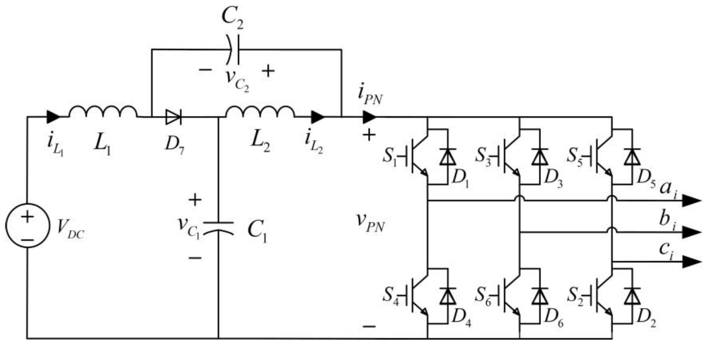
2.1. LVC-qZSI

The working modes of LVC-qZSI are divided into through state and non-through state, corresponding to whether the switching devices of the same bridge arm are turned on at the same time. The single module topology of LVC-qZSI is a three-phase qZSI, as shown in Figure 1.

In Figure 1, $C_1$, $C_2$, $L_1$, and $L_2$ are the Z-source network capacitances and inductances, $D_7$ is the DC diode, $S_1$ to $S_6$ represent six IGBTs, and $D_1$ to $D_6$ represent six freewheeling diodes. The small signal model is established in a switching period, as shown in Formula (1).

$$\{\begin{array}{l}{L}_1\frac{d{\hat{i}}_{L_1}}{dt}=\hat{d}\left(V_{C_1}+V_{C_2}\right)-\left(1-D\right){\hat{v}}_{C_1}+D{\hat{v}}_{C_2}\\ L_2\frac{d{\hat{i}}_{L_2}}{dt}=\hat{d}\left(V_{C_1}+V_{C_2}\right)-\left(1-D\right){\hat{v}}_{C_2}+D{\hat{v}}_{C_1}\\ C_1\frac{d{\hat{v}}_{C_1}}{dt}=\hat{d}\left(I_{PN}-I_{L_1}-I_{L_2}\right)+\left(1-D\right){\hat{i}}_{L_1}-\left(1-D\right){\hat{i}}_{PN}-D{\hat{i}}_{L_2}\\ C_2\frac{d{\hat{v}}_{C_2}}{dt}=\hat{d}\left(I_{PN}-I_{L_1}-I_{L_2}\right)+\left(1-D\right){\hat{i}}_{L_2}-\left(1-D\right){\hat{i}}_{PN}-D{\hat{i}}_{L_1}\end{array}$$

(1)

To simplify the calculation, it is assumed that the network parameters are symmetric, i.e., $C=C_1=C_2$ and $L=L_1=L_2$. When the parameters are symmetric, the corresponding small signals are also symmetric, i.e., ${\widehat{v}}_C={\widehat{v}}_{C_1}={\widehat{v}}_{C_2}$ and ${\widehat{i}}_L={\widehat{i}}_{L_1}={\widehat{i}}_{L_2}$. Transform Formula (1) into linear equations by the Laplace transformation, as shown in Formula (2):

$$\left[\begin{array}{l}{\widehat{i}}_L\left(s\right)\\ {\widehat{v}}_C\left(s\right)\end{array}\right]=\left[\begin{array}{l}\begin{array}{ccc}{G}_{{\widehat{v}}_{DC}}^{{\widehat{i}}_L}\left(s\right)& G_{{\widehat{i}}_{PN}}^{{\widehat{i}}_L}\left(s\right)& G_{\widehat{d}}^{{\widehat{i}}_L}\left(s\right)\end{array}\\ \begin{array}{ccc}{G}_{{\widehat{v}}_{DC}}^{{\widehat{v}}_C}\left(s\right)& G_{{\widehat{i}}_{PN}}^{{\widehat{v}}_C}\left(s\right)& G_{\widehat{d}}^{{\widehat{v}}_C}\left(s\right)\end{array}\end{array}\right]\left[\begin{array}{l}{\widehat{v}}_{DC}\left(s\right)\\ {\widehat{i}}_{PN}\left(s\right)\\ \widehat{d}\left(s\right)\end{array}\right]$$

(2)

where

$$\begin{array}{l}{G}_{{\widehat{i}}_{PN}}^{{\widehat{i}}_L}\left(s\right)=\frac{\left(1-D\right)\left(1-2D\right)}{LC{s}^2+{\left(1-2D\right)}^2}\\ G_{{\widehat{i}}_{PN}}^{{\widehat{v}}_C}\left(s\right)=\frac{-\left(1-D\right)Ls}{LC{s}^2+{\left(1-2D\right)}^2}\end{array}$$

(3)

LVC-qZSI is composed of three traditional three-phase qZSIs cascaded by line voltage. The main circuit topology is shown in Figure 2.

where $L_x$ is the cascaded inductance between modules; $L_f$ is the filter inductance; $e_A$, $e_B$, and $e_C$ are three-phase voltages of the grid. According to the LVC topology and Kirchhoff law, there is:

$$\{\begin{array}{l}{\dot{I}}_{ai}+{\dot{I}}_{bi}+{\dot{I}}_{ci}=0\\ {\dot{U}}_{AB}={\dot{U}}_{a1b1}+{\dot{U}}_{a2b2}+{\dot{U}}_{b1a2}=j\omega L_f{\dot{I}}_{b2}-j\omega L_f{\dot{I}}_{a1}+{\dot{E}}_{AB}\\ {\dot{U}}_{BC}={\dot{U}}_{b2c2}+{\dot{U}}_{b3c3}+{\dot{U}}_{c2b3}=j\omega L_f{\dot{I}}_{c3}-j\omega L_f{\dot{I}}_{b2}+{\dot{E}}_{BC}\\ {\dot{U}}_{CA}={\dot{U}}_{c3a3}+{\dot{U}}_{c1a1}+{\dot{U}}_{a3c1}=j\omega L_f{\dot{I}}_{a1}-j\omega L_f{\dot{I}}_{c3}+{\dot{E}}_{CA}\end{array}$$

(4)

The voltage and current of the cascaded network are assumed to be ${\dot{U}}_O$ and ${\dot{I}}_O$, respectively:

$$\{\begin{array}{l}{\dot{U}}_{a3b3}+{\dot{U}}_{b1c1}+{\dot{U}}_{c2a2}={\dot{U}}_{a3c1}+{\dot{U}}_{b1a2}+{\dot{U}}_{c2b3}={\dot{U}}_O\\ {\dot{I}}_{a3}+{\dot{I}}_{b1}+{\dot{I}}_{c2}=-j({\dot{U}}_O/\omega L_x)={\dot{I}}_O\end{array}$$

(5)

Substitute Formula (5) into Formula (4) to obtain Formula (6) and Formula (7):

$$\begin{array}{ccc}\{\begin{array}{l}{\dot{I}}_{a1}={\dot{I}}_A\hfill \\ {\dot{I}}_{b1}=\left(2{\dot{I}}_B+{\dot{I}}_C+{\dot{I}}_O\right)/3\hfill \\ {\dot{I}}_{c1}=\left({\dot{I}}_B+2{\dot{I}}_C-{\dot{I}}_O\right)/3\hfill \end{array}& \{\begin{array}{l}{\dot{I}}_{a2}=\left(2{\dot{I}}_A+{\dot{I}}_C-{\dot{I}}_O\right)/3\hfill \\ {\dot{I}}_{b2}={\dot{I}}_B\hfill \\ {\dot{I}}_{c2}=\left({\dot{I}}_A+2{\dot{I}}_C+{\dot{I}}_O\right)/3\hfill \end{array}& \{\begin{array}{l}{\dot{I}}_{a3}=\left(2{\dot{I}}_A+{\dot{I}}_B+{\dot{I}}_O\right)/3\hfill \\ {\dot{I}}_{b3}=\left({\dot{I}}_A+2{\dot{I}}_B-{\dot{I}}_O\right)/3\hfill \\ {\dot{I}}_{c3}={\dot{I}}_C\hfill \end{array}\end{array}$$

(6)

$$\{\begin{array}{l}{\dot{U}}_{a1b1}+{\dot{U}}_{a2b2}+{\dot{U}}_O/3={\dot{E}}_{AB}-\left[{\mathrm{R}}_{\mathrm{f}}+j\omega \left(L_f+L_x/3\right)\right]\left({\dot{I}}_B-{\dot{I}}_A\right)\hfill \\ {\dot{U}}_{b2c2}+{\dot{U}}_{b3c3}+{\dot{U}}_O/3={\dot{E}}_{BC}-\left[{\mathrm{R}}_{\mathrm{f}}+j\omega \left(L_f+L_x/3\right)\right]\left({\dot{I}}_C-{\dot{I}}_B\right)\hfill \\ {\dot{U}}_{c3a3}+{\dot{U}}_{c1a1}+{\dot{U}}_O/3={\dot{E}}_{CA}-\left[{\mathrm{R}}_{\mathrm{f}}+j\omega \left(L_f+L_x/3\right)\right]\left({\dot{I}}_A-{\dot{I}}_C\right)\hfill \end{array}$$

(7)

The calculation results of instantaneous voltage and instantaneous current are shown in Formula (8) and Formula (9), respectively.

$$\{\begin{array}{l}{u}_{a1O1}=u_{a2O2}=u_{a3O3}=\sqrt{2}U\sin (\omega t-\phi )\\ u_{b1O1}=u_{b2O2}=u_{b3O3}=\sqrt{2}U\sin (\omega t-{120}^{\circ }-\phi )\\ u_{c1O1}=u_{c2O2}=u_{c3O3}=\sqrt{2}U\sin (\omega t+{120}^{\circ }-\phi )\end{array}$$

(8)

$$\begin{array}{ccc}\{\begin{array}{l}{i}_{a1}=\sqrt{2}I\sin (\omega t)\\ i_{b1}=\sqrt{2}I/\sqrt{3}\sin (\omega t-{150}^{\circ })\\ i_{c1}=\sqrt{2}I/\sqrt{3}\sin (\omega t+{150}^{\circ })\end{array}& \{\begin{array}{l}{i}_{a2}=\sqrt{2}I/\sqrt{3}\sin (\omega t+{30}^{\circ })\\ i_{b2}=\sqrt{2}I\sin (\omega t-{120}^{\circ })\\ i_{c2}=\sqrt{2}I/\sqrt{3}\sin (\omega t+{90}^{\circ })\end{array}& \{\begin{array}{l}{i}_{a3}=\sqrt{2}I/\sqrt{3}\sin (\omega t-{30}^{\circ })\\ i_{b3}=\sqrt{2}I/\sqrt{3}\sin (\omega t-{90}^{\circ })\\ i_{c3}=\sqrt{2}I\sin (\omega t+{120}^{\circ })\end{array}\end{array}$$

(9)

Formula (8) shows that the output voltage vectors of three modules differ by 120° and are three-phase symmetrical. Formula (9) shows that the current vectors are not three-phase symmetrical, the lengths of output current vectors ${\stackrel{•}{I}}_{a1}$, ${\stackrel{•}{I}}_{b2}$, and ${\stackrel{•}{I}}_{c3}$ are $\sqrt{3}$ times the lengths of cascaded current vectors. The angle between the output current vector and cascaded current vector is 150°, and the angle between the cascaded current vectors is 60°. Three-phase current vectors are shown in Figure 3.

According to the calculation of active power, the instantaneous expression of output power of each module and total output power can be obtained as follows:

$$\{\begin{array}{l}{p}_1=u_{a1O1}{i}_{a1}+u_{b1O1}{i}_{b1}+u_{c1O1}{i}_{c1}=2UI\cos \phi -UI\cos (2\omega t-\phi )\\ p_2=u_{a2O2}{i}_{a2}+u_{b2O2}{i}_{b2}+u_{c2O2}{i}_{c2}=2UI\cos \phi -UI\cos (2\omega t+120°-\phi )\\ p_3=u_{a3O3}{i}_{a3}+u_{b3O3}{i}_{b3}+u_{c3O3}{i}_{c3}=2UI\cos \phi -UI\cos (2\omega t-120°-\phi )\\ p=p_1+p_2+p_3=6UI\cos \phi \end{array}$$

(10)

2.2. Performance Index

2.2.1. Double Frequency Voltage Ripple Ratio

Formula (10) shows that the total instantaneous power of LVC-qZSI is constant, and there is a double frequency component in the instantaneous power of each module, which makes the capacitance voltage and inductance current in each module produce double frequency fluctuation. To a certain extent, the parameter optimization of LVC-qZSI can restrain the double frequency fluctuation and improve the stability of the system.

Take the capacitance voltage as an example. According to reference [17], the small signal model analysis result of the DC side current in the LVC-qZSI network is as follows:

$${\widehat{i}}_{PN}=-\frac{2\left(1-2D\right)UI}{\left(1-D\right)V_{DC}}\cos \left(2\omega t-\alpha \right)$$

(11)

where

$$\alpha =\phi +\arctan \frac{4\omega L{I}_{PN}\left(1-D\right)\left(1-2D\right)}{\left[4{\omega }^{2}LC-{\left(1-2D\right)}^2\right]V_{DC}}$$

(12)

According to Formula (2), the double frequency ripple of capacitance voltage is as follows:

$${\widehat{v}}_C\left(s\right)=G_{{\widehat{v}}_{DC}}^{{\widehat{v}}_C}\left(s\right){\widehat{v}}_{DC}\left(s\right)+G_{{\widehat{i}}_{PN}}^{{\widehat{v}}_C}\left(s\right){\widehat{i}}_{PN}\left(s\right)+G_{\widehat{d}}^{{\widehat{v}}_C}\left(s\right)\widehat{d}\left(s\right)$$

(13)

According to Formula (3), the calculation result of the double frequency voltage ripple of capacitance $C_1$ is shown in Formula (14):

$${\widehat{v}}_{C_1}=\frac{4\omega LUI\left(1-2D\right)}{\left[4{\omega }^{2}LC-{\left(1-2D\right)}^2\right]V_{DC}}\sin \left(2\omega t-\alpha \right)$$

(14)

The average value of DC voltage of capacitance $C_1$ is:

$$V_{C_1}=\frac{1-D}{1-2D}{V}_{DC}$$

(15)

Take the double frequency voltage ripple ratio of capacitance $C_1$ as the optimization objective function, as shown in Formula (16):

$$R_{C_1}=\frac{\left|{\widehat{v}}_{C_1}\right|}{V_{C_1}}\times 100\%=\frac{4\omega LUI{\left(1-2D\right)}^2}{\left[4{\omega }^{2}LC-{\left(1-2D\right)}^2\right]\left(1-D\right)V_{DC}^2}\times 100\%$$

(16)

Similarly, take the double frequency voltage ripple ratio of capacitance $C_2$ as another optimization objective function, as shown in Formula (17):

$$R_{C_2}=\frac{\left|{\widehat{i}}_{L_1}\right|}{I_{L_1}}\times 100\%=\frac{4\omega LUI{\left(1-2D\right)}^2}{\left[4{\omega }^{2}LC-{\left(1-2D\right)}^2\right]D{V}_{DC}^2}\times 100\%$$

(17)

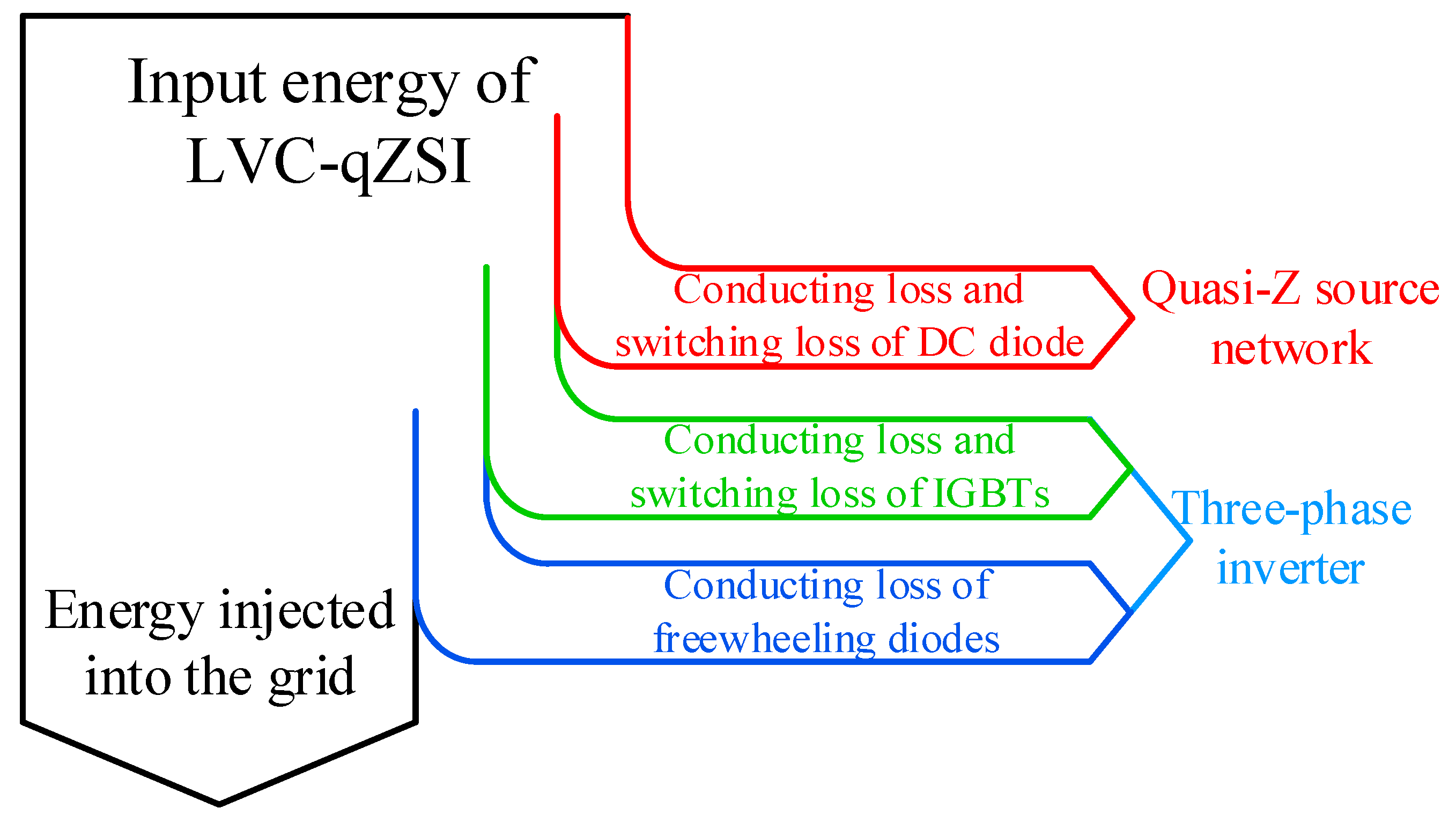
2.2.2. Power Loss Ratio

The LVC-qZSI power loss mainly includes conducting loss and switching loss, which is generated by IGBTs, DC diodes, and freewheeling diodes. The power loss is determined by circuit parameters and can be reduced. The energy flow of LVC-qZSI is shown in Figure 4.

Figure 4 describes the input energy to the output energy of LVC-qZSI. Meanwhile, the energy loss is classified in detail. Take the power loss in a single module of LVC-qZSI as the performance index:

$$P_{Loss}={\displaystyle \sum _{n=1}^6\left(P_C^{IGB{T}_n}+P_S^{IGB{T}_n}+P_C^{Diod{e}_n}\right)}+P_C^{D_7}+P_S^{D_7}$$

(18)

where $P_C^{IGBT}$ represents the conducting loss of one IGBT; $P_S^{IGBT}$ and $P_S^{D_7}$ represent switching loss of one IGBT and DC diode $D_7$, respectively; $P_C^{Diode}$ and $P_C^{D_7}$ represent conducting loss of one freewheeling diode and DC diode $D_7$, respectively.

According to references [18] and [19], we can get the conducting loss of IGBTs and freewheeling diodes as shown in Formula (19) and Formula (20), respectively:

$${\displaystyle \sum _{n=1}^6{P}_C^{IGB{T}_n}}=\left(\frac{5}{6}+\frac{20M}{9\pi }\right)\frac{V_{CEN}-V_{CEO}}{I_{CN}}{I}^2+\left(3\sqrt{2}+2\sqrt{6}\right)\left[\frac{1}{3\pi }+\frac{M}{12}\right]V_{CEO}I+\left(12I_L\frac{V_{CEN}-V_{CEO}}{I_{CN}}+6V_{CEO}\right)I_{L}D$$

(19)

$${\displaystyle \sum _{n=1}^6{P}_C^{Diod{e}_n}}=\left(\frac{5}{6}-\frac{20M}{9\pi }\right)\frac{V_{FN}-V_{FO}}{I_{CN}}{I}^2+\left(3\sqrt{2}+2\sqrt{6}\right)\left[\frac{1}{3\pi }-\frac{M}{12}\right]V_{FO}I$$

(20)

where $V_{CEO}$ is the saturation voltage drop, $I_{CN}$ is the rated current, and $V_{CEN}$ is the collector-to-emitter voltage at rated current. Meanwhile, $V_{FO}$ is the saturation voltage drop, $V_{FN}$ is the diode voltage drop at rated current, $D$ is the shoot-through duty cycle, $M$ is the modulation index, and $I_L$ is the inductance current.

The switching loss is proportional to the switching frequency, and the switching loss of IGBTs is shown in Formula (21):

$${\displaystyle \sum _{n=1}^6{P}_S^{IGB{T}_n}}=\left(2V_C-V_{DC}\right)f_S\left[\frac{12I_L{}^2{t}_{rN}}{I_{CN}}+4I_L\left(1+\frac{I_L}{I_{CN}}\right)t_{fN}+2.4t_{rrN}\left(2+\frac{I_L}{I_{CN}}\right)\left(0.35I_{rrN}+0.3\frac{I_L}{I_{CN}}{I}_{rrN}+2I_L\right)\right]$$

(21)

where $t_{rN}$ is the rated rise time at rated current, $t_{fN}$ is the rated fall time at rated current, $t_{rrN}$ is the recovery time at rated current, $I_{rrN}$ is the recovery current, and $f_S$ is the switching frequency.

The conducting loss and switching loss of DC diodes are shown in Formula (22) and Formula (23), respectively:

$$P_C^{D_7}=\left(\frac{V_{FN}^{\prime }-V_{FO}^{\prime }}{I_{CN}^{\prime }}{I}_{in}+V_{FO}^{\prime }\right)I_{in}\left(1-D\right)$$

(22)

$$P_S^{D_7}=q_{rr}{V}_R{f}_S$$

(23)

The power loss ratio $R_{Loss}$ represents the ratio of the power loss to the input power of LVC-qZSI, which is taken as the third optimization objective function:

$$R_{Loss}=\frac{P_{Loss}}{P_{In}}$$

(24)

where $P_{In}$ represents the input power of LVC-qZSI.

At the same time, the energy conversion efficiency $\eta$ represents the ratio of the effective output power to the input power of LVC-qZSI [20]:

$$\eta =1-R_{Loss}$$

(25)

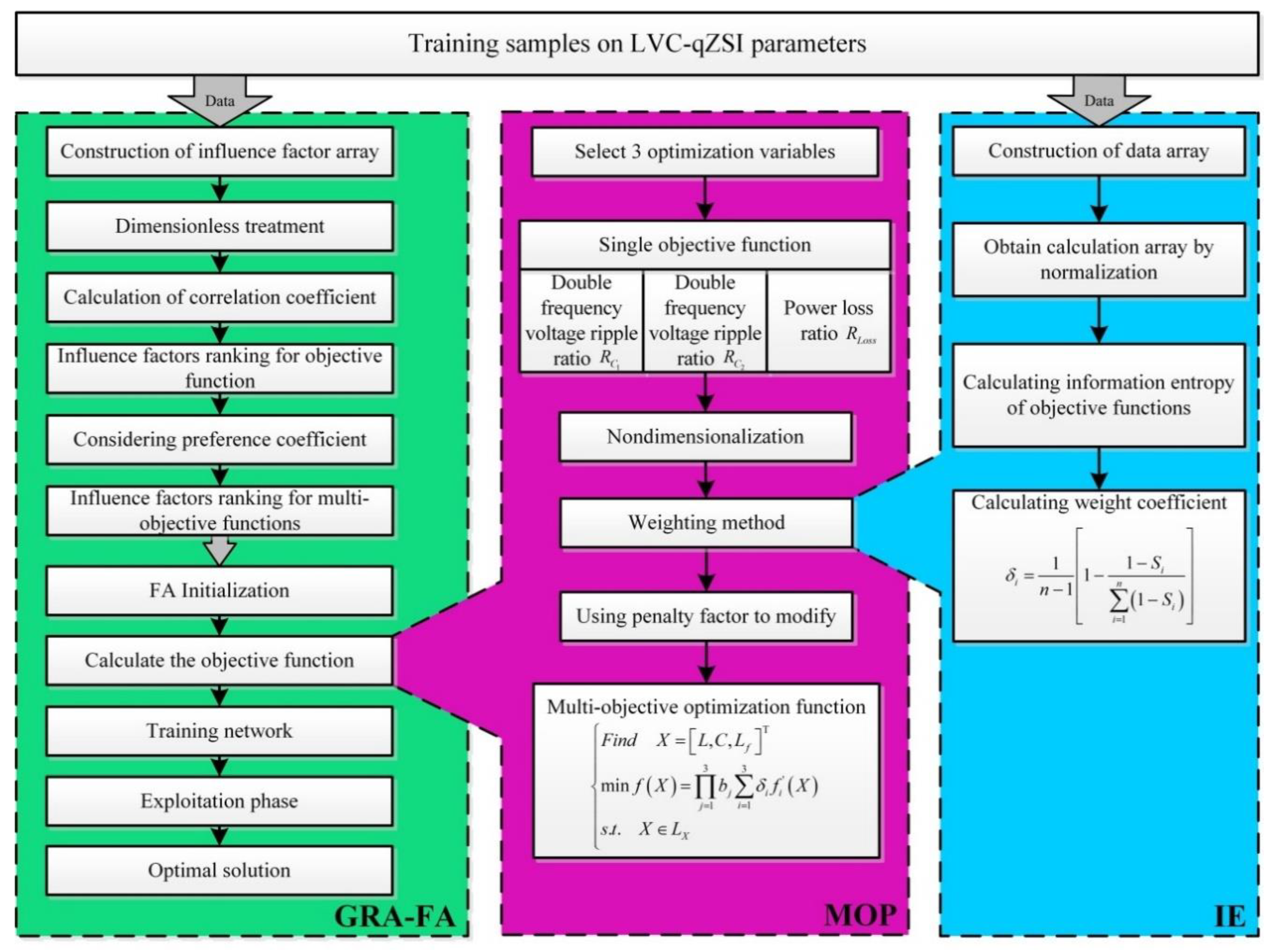
3. GRA of LVC-qZSI Parameters

3.1. Description

As LVC-qZSI is a nonlinear, multi-parameter, and strong coupling dynamic system, its optimization objectives are affected by many optimization variables, such as Z-source network inductance, Z-source network capacitance, filter inductance, etc. Since there are multiple optimization variables and the coupling relationship between optimization objectives is too strong, it is difficult to accurately calculate the influence effect of each optimization variable when establishing the optimization model. Therefore, it is necessary to analyze and sort all the influence factors by using GRA according to the recorded data in previous experiments. On this basis, we can select the main influence factors and discard the secondary ones, so as to reduce the complexity of the system and establish the basis for subsequent parameter optimization.

In GRA, the main influence factors and secondary ones leading to the development of the system are determined by analyzing the relationship between various influence factors and reference indexes. For example, in order to optimize the parameters of LVC-qZSI, we can take the double frequency voltage ripple ratio $R_{C_1}$ (%) as the reference index column and expressed by $X_0={\left[x_0\left(1\right),x_0\left(2\right),x_0\left(3\right),\cdots ,x_0\left(j\right)\cdots ,x_0\left(k\right)\right]}^T,\left(j=1,2,\cdots ,k\right)$, where $k$ is the capacity of the selected training samples. The larger the training sample size is, the smaller the random errors in the samples are, and the more accurate the analysis results of GRA are. In the process of analyzing the LVC-qZSI model, the reference index column $X_0$ is affected by various parameters in the circuit. To describe the characteristics of LVC-qZSI in detail, six circuit parameters are selected as influence factors columns (represented by $X_1$, $X_2$, $X_3$, $X_4$, $X_5$, and $X_6$, respectively), including Z-source network inductance $L$($\mathsf{\mu }\mathrm{H}$), Z-source network capacitance $C$($\mathsf{\mu }\mathrm{F}$), filter inductance $L_f$($\mathrm{mH}$), cascaded inductance $L_x$($\mathrm{mH}$), modulation index $M$, and shoot-through duty cycle $D$. The circuit parameters are shown in

Table 1. LVC-qZSI circuit parameters.

Symbol	Definition	Value Range	Unit
$L$	Z-source network inductance	450–2000	$\mathsf{\mu }\mathrm{H}$
$C$	Z-source network capacitance	300–1500	$\mathsf{\mu }\mathrm{H}$
$L_f$	Filter inductance	0.50–20	$\mathrm{mH}$
$L_x$	Cascaded inductance	0.50–20	$\mathrm{mH}$
$M$	Modulation index	0.50–1.00
$D$	Shoot-through duty cycle	0.05–0.40

.

3.2. Sorting of LVC-qZSI Parameters Based on GRA

In order to obtain accurate training samples, our research team built a LVC-qZSI circuit system in MATLAB/Simulink, as shown in Figure 5. In the simulation model, we encapsulate each functional module, including Control System, DC Source, Z-Source Network, Inverter Bridge, and Filter. Specifically, Control System is used to change the modulation index $M$ and shoot-through duty cycle $D$; DC Source contains a DC voltage source; Z-Source Network is an encapsulation of boost network; Inverter Bridge mainly includes a three-phase inverter bridge, which is composed of six IGBTs and six freewheeling diodes; Filter is an encapsulation of filter inductance $L_f$.

Set the training sample size as 30, and randomly adjust the values of Z-source network inductance, Z-source network capacitance, filter inductance, cascaded inductance, modulation index and shoot-through duty cycle, and ensure that they are within the range specified in Table 1. The recorded influence factors columns (from $X_1$ to $X_6$) and reference index column $X_0$ are shown in

Table 2. Values of LVC-qZSI parameters.

${\mathit{X}}_0$	LVC-qZSI Parameters
	${\mathit{X}}_1$	${\mathit{X}}_2$	${\mathit{X}}_3$	${\mathit{X}}_4$	${\mathit{X}}_5$	${\mathit{X}}_6$
7.17	200	200	12	10	0.69	0.16
13.33	300	250	6	16	0.52	0.37
0.88	400	300	5	7	0.75	0.09
0.59	420	300	2	3	0.90	0.14
9.77	500	400	10	9	0.70	0.33
12.73	550	500	5	11	0.72	0.30
3.39	600	1300	4	14	0.82	0.19
0.12	640	850	3	5	0.55	0.15
2.23	680	700	12	9	0.67	0.22
4.34	700	600	15	12	0.77	0.25
2.06	750	1300	7	6	0.61	0.27
5.06	800	700	13	10	0.75	0.30
11.89	830	300	10	8	0.82	0.35
10.40	880	500	8	10	0.71	0.32
1.79	920	1070	16	7	0.74	0.22
1.70	960	950	12	11	0.66	0.24
5.05	1000	800	8	15	0.65	0.35
8.99	1080	400	6	9	0.59	0.31
4.86	1150	760	10	6	0.56	0.38
3.90	1200	900	12	13	0.60	0.40
1.97	1260	1000	6	10	0.64	0.23
1.82	1300	1100	17	8	0.80	0.20
3.85	1350	1000	10	4	0.78	0.22
11.59	1470	400	5	9	0.55	0.36
2.23	1500	1200	11	5	0.85	0.15
2.02	1550	800	13	8	0.63	0.26
0.92	1600	1400	9	11	0.55	0.28
5.26	1640	900	10	16	0.83	0.35
5.03	1750	1050	8	4	0.88	0.18
0.03	1800	1500	6	7	0.57	0.10

.

In GRA, it is difficult to compare and get accurate results due to the different dimensions of the six influence factors. Therefore, to ensure the unity in quantity, the above data need to be dimensionless, as shown in Formula (26):

$$x^{\ast }{}_i\left(j\right)=\frac{x_i\left(j\right)}{\frac{1}{k}{\displaystyle \sum _{j=1}^k{x}_i\left(j\right)}},\left(i=0,1,\cdots ,m,j=1,2,\cdots ,k\right)$$

(26)

where $m$ represents the number of influence factors and takes six. Meanwhile, $k$ represents the capacity of the training samples and takes 30. The dimensionless matrix is obtained after dimensionless treatment, as shown in

Table 3. Dimensionless matrix of LVC-qZSI parameters.

${\mathit{X}}_0{}^{*}$	LVC-qZSI Parameters
	${\mathit{X}}_1{}^{*}$	${\mathit{X}}_2{}^{*}$	${\mathit{X}}_3{}^{*}$	${\mathit{X}}_4{}^{*}$	${\mathit{X}}_5{}^{*}$	${\mathit{X}}_6{}^{*}$
1.4838	0.2015	0.2561	1.3284	1.0989	0.9923	0.6258
2.7585	0.3022	0.3201	0.6642	1.7582	0.7478	1.4472
0.1821	0.4030	0.3841	0.5535	0.7692	1.0786	0.3520
0.1221	0.4231	0.3841	0.2214	0.3297	1.2943	0.5476
2.0218	0.5037	0.5122	1.1070	0.9890	1.0067	1.2907
2.6343	0.5541	0.6402	0.5535	1.2088	1.0355	1.1734
0.7015	0.6044	1.6645	0.4428	1.5385	1.1793	0.7432
0.0248	0.6447	1.0883	0.3321	0.5495	0.7910	0.5867
0.4615	0.6850	0.8963	1.3284	0.9890	0.9636	0.8605
0.8981	0.7052	0.7682	1.6605	1.3187	1.1074	0.9778
0.4263	0.7555	1.6645	0.7749	0.6593	0.8773	1.0561
1.0471	0.8059	0.8963	1.4391	1.0989	1.0786	1.1734
2.4605	0.8361	0.3841	1.1070	0.8791	1.1793	1.3690
2.1522	0.8865	0.6402	0.8856	1.0989	1.0211	1.2516
0.3704	0.9268	1.3700	1.7712	0.7692	1.0642	0.8605
0.3518	0.9671	1.2164	1.3284	1.2088	0.9492	0.9387
1.0450	1.0074	1.0243	0.8856	1.6484	0.9348	1.3690
1.8604	1.0880	0.5122	0.6642	0.9890	0.8485	1.2125
1.0057	1.1585	0.9731	1.1070	0.6593	0.8054	1.4863
0.8071	1.2089	1.1524	1.3284	1.4286	0.8629	1.5645
0.4077	1.2693	1.2804	0.6642	1.0989	0.9204	0.8996
0.3766	1.3096	1.4085	1.8819	0.8791	1.1505	0.7823
0.7967	1.3600	1.2804	1.1070	0.4396	1.1218	0.8605
2.3984	1.4809	0.5122	0.5535	0.9890	0.7910	1.4081
0.4615	1.5111	1.5365	1.2177	0.5495	1.2224	0.5867
0.4180	1.5615	1.0243	1.4391	0.8791	0.9060	1.0169
0.1904	1.6118	1.7926	0.9963	1.2088	0.7910	1.0952
1.0885	1.6521	1.1524	1.1070	1.7582	1.1937	1.3690
1.0409	1.7629	1.3444	0.8856	0.4396	1.2656	0.7040
0.0062	1.8133	1.9206	0.6642	0.7692	0.8198	0.3911

.

After calculating the dimensionless reference index column $X_0{}^{\ast }$ and dimensionless influence factors columns $X_i{}^{\ast }$, the correlation coefficient of six influence factors is shown in Formula (27):

$${\xi }_i\left(j\right)=\frac{\underset{i}{\min }\underset{j}{\min }\left|x_0{}^{\ast }\left(j\right)-x_i{}^{\ast }\left(j\right)\right|+\rho \underset{i}{\max }\underset{j}{\max }\left|x_0{}^{\ast }\left(j\right)-x_i{}^{\ast }\left(j\right)\right|}{\left|x_0{}^{\ast }\left(j\right)-x_i{}^{\ast }\left(j\right)\right|+\rho \underset{i}{\max }\underset{j}{\max }\left|x_0{}^{\ast }\left(j\right)-x_i{}^{\ast }\left(j\right)\right|},\left(i=1,2,\cdots ,6;j=1,2,\cdots ,30\right)$$

(27)

where $\rho$ is the resolution coefficient, and its value is in the range of [0,1], which usually takes 0.5. After calculating the correlation coefficient, the correlation coefficient matrix is obtained, as shown in

Table 4. Correlation coefficient matrix of LVC-qZSI parameters.

${\mathit{\xi }}_1$	${\mathit{\xi }}_2$	${\mathit{\xi }}_3$	${\mathit{\xi }}_4$	${\mathit{\xi }}_5$	${\mathit{\xi }}_6$
0.4966	0.5076	0.9011	0.7729	0.7250	0.5976
0.3384	0.3400	0.3752	0.5594	0.3849	0.4909
0.8604	0.8717	0.7794	0.6868	0.5868	0.8917
0.8153	0.8366	0.9391	0.8683	0.5194	0.7539
0.4539	0.4554	0.5818	0.5514	0.5557	0.6363
0.3768	0.3869	0.3767	0.4698	0.4410	0.4636
0.9407	0.5689	0.8384	0.6037	0.7308	0.9818
0.6746	0.5440	0.8119	0.7113	0.6251	0.6964
0.8588	0.7497	0.5950	0.7101	0.7205	0.7662
0.8773	0.9180	0.6263	0.7561	0.8673	0.9532
0.8005	0.5055	0.7906	0.8532	0.7424	0.6710
0.8484	0.9040	0.7695	0.9740	0.9897	0.9204
0.4370	0.3773	0.4829	0.4437	0.4968	0.5374
0.4999	0.4550	0.4997	0.5464	0.5284	0.5856
0.6986	0.5596	0.4742	0.7663	0.6486	0.7256
0.6763	0.5957	0.5654	0.5979	0.6829	0.6868
0.9849	0.9982	0.8984	0.6807	0.9315	0.8032
0.6232	0.4839	0.5142	0.5938	0.5565	0.6645
0.9028	0.9888	0.9377	0.7918	0.8727	0.7296
0.7648	0.7923	0.7126	0.6740	0.9709	0.6278
0.5965	0.5934	0.8397	0.6495	0.7161	0.7248
0.5769	0.5516	0.4561	0.7203	0.6227	0.7630
0.6959	0.7283	0.8103	0.7864	0.8026	0.9650
0.5810	0.4003	0.4057	0.4727	0.4396	0.5619
0.5473	0.5413	0.6282	0.9472	0.6267	0.9211
0.5257	0.6796	0.5543	0.7380	0.7264	0.6823
0.4705	0.4405	0.6129	0.5549	0.6817	0.5845
0.6958	0.9649	1.0000	0.6569	0.9350	0.8264
0.6393	0.8139	0.9011	0.6814	0.8581	0.7966
0.4107	0.3967	0.6610	0.6261	0.6106	0.7728

.

The grey correlation matrix is used to analyze the advantages of the influence factors, and the average value of the correlation coefficient is defined as the correlation degree, as shown below:

$$r_i=\frac{1}{k}{\displaystyle \sum _{j=1}^k{\xi }_i\left(j\right)}$$

(28)

where $r_i\in \left(0,1\right)$, which means that any influence factor is not strictly independent of $R_{C_1}$, and it is not the only strict determinant factor. If $l,j\in \left\{1,2,\cdots ,m\right\}$ and $r_l\ge r_j$, it means $X_i$ is better than $X_j$.

This paper compares the correlation degrees between the reference index column and the influence factors columns. The comparison results show that the shoot-through duty cycle (0.7261) has the greatest influence on $R_{C_1}$, followed by the modulation index (0.6866), cascaded inductance (0.6815), filter inductance (0.6780), and Z-source network inductance (0.6556). The Z-source network capacitance has the least influence with the correlation degree of 0.6316. According to the correlation degrees, the main influence factors are shoot-through duty cycle, modulation index, and cascaded inductance.

Similarly, take the voltage ripple ratio $R_{C_2}$ and power loss ratio $R_{Loss}$ as the reference indexes columns, the correlation degrees between the reference indexes columns and the influence factors columns are calculated and summarized in

Table 5. Correlation degrees of LVC-qZSI parameters.

Reference Index	Influence Factors
	${\mathit{X}}_1$	${\mathit{X}}_2$	${\mathit{X}}_3$	${\mathit{X}}_4$	${\mathit{X}}_5$	${\mathit{X}}_6$
$R_{C_1}$	0.6556	0.6316	0.6780	0.6815	0.6866	0.7261
$R_{C_2}$	0.7789	0.8254	0.6811	0.7461	0.6609	0.7926
$R_{Loss}$	0.9573	0.9498	0.8692	0.8045	0.5098	0.5237

.

The results of GRA indicate that $R_{C_1}$, $R_{C_2}$, and $R_{Loss}$ are affected by LVC-qZSI parameters to varying degrees. For example, the main influence factors of $R_{C_2}$ are Z-source network capacitance (0.8254), shoot-through duty cycle (0.7926), and Z-source network inductance (0.7789); the main influence factors of $R_{Loss}$ are Z-source network inductance (0.9573), Z-source network capacitance (0.9498), and filter inductance (0.8692). In order to reasonably evaluate the comprehensive influence of each LVC-qZSI parameter on the three optimization objective functions, this paper introduces ${\alpha }_1$, ${\alpha }_2$, and ${\alpha }_3$ as the preference coefficients of $R_{C_1}$, $R_{C_2}$, and $R_{Loss}$, respectively, then adjusts the value of ${\alpha }_i$ according to the decision-maker’s preference and specific decision-making conditions. To simplify the calculation, it is assumed that the preference coefficients of $R_{C_1}$ and $R_{C_2}$ are the same (i.e., ${\alpha }_1={\alpha }_2$) and satisfies ${\displaystyle \sum _{i=1}^3{\alpha }_i}=1$. In other words, ${\alpha }_1={\alpha }_2=\alpha$ and ${\alpha }_3=1-2\alpha$. Set the step size of $\alpha$ to 0.05, and the value range is 0 to 1. The comprehensive correlation degrees between LVC-qZSI parameters and optimization objective functions is shown in Figure 6.

The abscissa is the value of $\alpha$ and the ordinate is the comprehensive correlation degree. The six lines in Figure 6 represent ${\displaystyle \sum _{i=1}^3{\alpha }_i}{X}_j\left(j=1,2,\cdots ,6\right)$. The analysis results of Figure 6 are as follows:

(1)

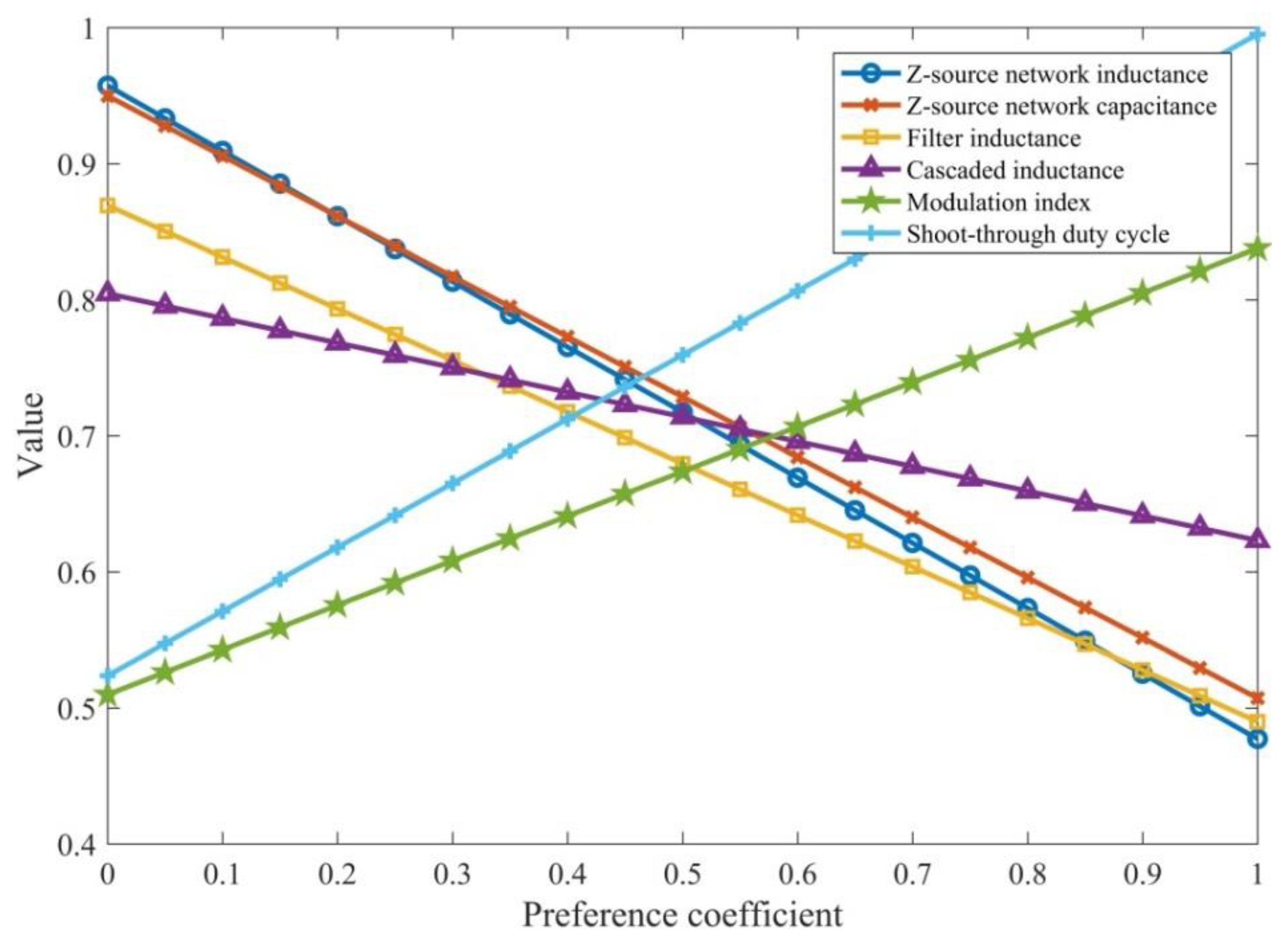
For the value range of preference coefficient $\alpha$, with the increase of $\alpha$, the main influence factors are constantly changing. When $\alpha \in \left[0,0.30\right]$, Z-source network inductance, Z-source network capacitance, and filter inductance have the greatest influence on objective functions; when $\alpha \in \left(0.30,0.43\right]$, Z-source network inductance, Z-source network capacitance, and cascaded inductance are selected as main influence factors; when $\alpha \in \left(0.43,0.58\right]$, the results of influence factors are complex and confusing, which need to be analyzed according to the specific situation; when $\alpha \in \left(0.58,1.00\right]$, shoot-through duty cycle, modulation index, and cascaded inductance have the greatest influence;

(2)

For the trend, the correlation degrees of Z-source network inductance, Z-source network capacitance, filter inductance, and cascaded inductance are negatively correlated with preference coefficient $\alpha$; the correlation degrees of modulation index and shoot-through duty cycle are positively correlated with preference coefficient $\alpha$;

(3)

When the power loss is not considered, the influence of circuit device parameters (including Z-source network inductance, Z-source network capacitance, filter inductance, and cascaded inductance) on the comprehensive correlation degrees is obvious; when the power loss is considered, the influence of circuit control parameters (including shoot-through duty cycle and modulation index) is obvious.

4. Integration Optimization Strategy of LVC-qZSI Parameters Based on GRA-FA

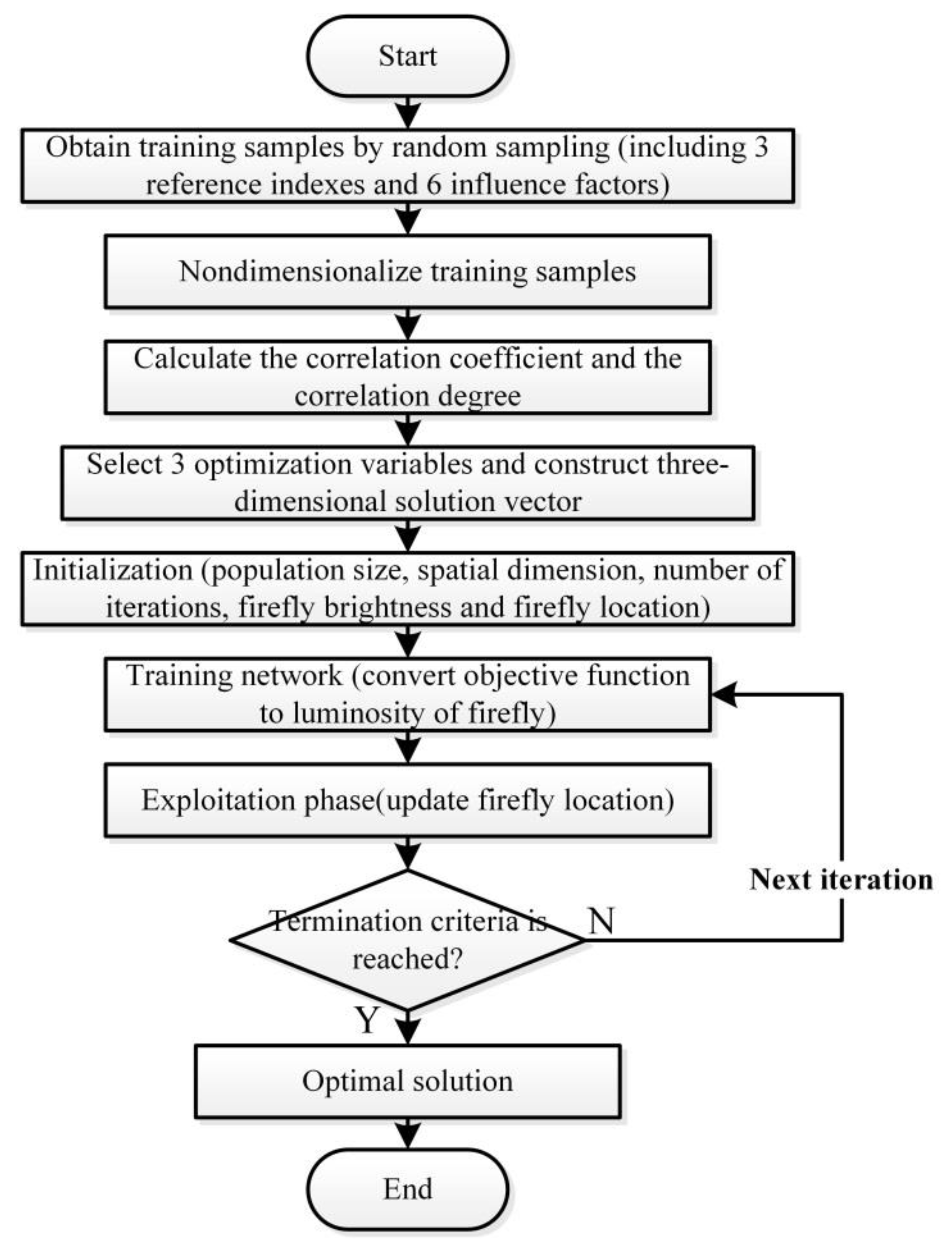
Compared with single objective optimization, multi-objective optimization is more difficult and complex because it needs to optimize multiple objective functions at the same time. There are conflicts among multiple optimization objectives, and the improvement of one objective may cause the performance degradation of other objectives. For the multi-objective optimization of LVC-qZSI parameters, this paper combines GRA in Section 3 and FA, simplifies the optimization variables according to the selecting results of GRA, and then proposes the multi-objective optimization model of LVC-qZSI parameters, so as to obtain the optimal solution of LVC-qZSI parameters.

4.1. GRA-FA

Based on the simulation and simplification of firefly population behavior, Yang proposed the firefly algorithm, which is a heuristic algorithm for swarm intelligence optimization. Due to its strong local search capability and robustness, FA is used to solve multi-objective optimization problems. In FA, each firefly represents a candidate solution in the D-dimensional search space and randomly distributes in the solution space. Due to the attraction between each other, after multiple moves, all individuals will gather in the position of the brightest firefly, so as to realize the optimization.

In FA, to ensure the diversity of population and enhance the global search ability of the algorithm, the initial positions of fireflies are randomly generated. Each firefly emits its fluorescence, and the brightness of the fluorescence is proportional to the value of the objective function. For a typical maximization problem, the relationship between the brightness $I\left(X\right)$ of the firefly $X$ and the objective function $f\left(X\right)$ can be expressed as $I\left(X\right)\propto f\left(X\right)$ [21].

In FA, every firefly is attracted to the one having comparatively greater brightness and its velocity is based on attractiveness [22]. The attractiveness of fireflies is determined by the luminosity of its fluorescence and is related to distance $r$. As the distance increases, the attractiveness decreases. The attractiveness $\beta$ of firefly is defined as:

$$\beta ={\beta }_0{e}^{-\gamma r_{ij}{}^2}$$

(29)

where ${\beta }_0$ is the attractiveness of the light source; $\gamma$ is the absorption coefficient of the light intensity and the theoretical value range is $\left[0,\infty \right)$, assumed to be a constant; $r_{ij}$ is the distance between $X_i$ (for firefly $i$) and $X_j$ (for firefly $j$), which can be expressed by the Cartesian distance:

$$r_{ij}=\Vert X_i-X_j\Vert =\sqrt{{\displaystyle \sum _{d=1}^D{\left(x_{id}-x_{jd}\right)}^2}}$$

(30)

where $D$ represents the dimension of the solution space, $x_{id}$ and $x_{jd}$ represent the element $d$ of $X_i$ and $X_j$, respectively.

Compare $X_i$ with $X_j$. If $I\left(X_i\right)<I\left(X_j\right)$, $X_i$ will move to $X_j$ with greater brightness due to attractiveness. The definition of position update is as follows:

$$x_{id}\left(t+1\right)=x_{id}\left(t\right)+{\beta }_0{e}^{-\gamma r_{ij}{}^2}\left[x_{jd}\left(t\right)-x_{id}\left(t\right)\right]+\alpha \left({\epsilon }_i-0.5\right)$$

(31)

If no firefly with greater brightness is found, $X_i$ will move randomly and its position will be updated to:

$$x_{id}\left(t+1\right)=x_{id}\left(t\right)+\alpha \left({\epsilon }_i-0.5\right)$$

(32)

where $\alpha$ represents the step factor and $\alpha \in \left[0,1\right]$; ${\epsilon }_i$ is a random number vector generated by Gaussian distribution, uniform distribution or other distributions and ${\epsilon }_i\in \left[0,1\right]$.

In Section 3.2, we use GRA to sort six parameters that affect the double frequency voltage ripple ratio and power loss ratio. After the preference coefficient is introduced, three main influence factors with the greatest comprehensive correlation degrees are selected to construct the solution vector of FA, and GRA-FA is proposed. Compared with the traditional FA, GRA-FA can reduce the number of optimization variables. In this way, the complexity of multi-objective optimization is greatly reduced, and the calculation speed is increased. The flowchart of GRA-FA is shown in Figure 7.

The main flow of GRA-FA is as follows (a–h):

• Set the sample size to 30 and randomly adjust the values of six circuit parameters in LVC-qZSI to obtain training samples (including three reference indexes and six influence factors);
• Nondimensionalize the training samples;
• Calculate the correlation degrees between three reference indexes and six influence factors;
• By introducing the preference coefficient, three main influence factors are selected as optimization variables, and the three-dimensional solution vector is constructed;
• Set the population size, the total number of iterations, and the spatial dimension, then randomly initialize the individual position and the fluorescence brightness of the fireflies;
• Train the network and transform the objective functions into the fluorescence brightness of fireflies;
• Exploitation phase (update fireflies locations);
• Judge whether the number of iterations reaches the upper limit. If the upper limit is reached, the optimal solution will be output; otherwise, return to step f for the next iteration.

4.2. Multi-Objective Optimization

Multi-objective optimization is a mathematical optimization problem in which more than one objective function is optimized simultaneously in a given region, and multiple objective functions are contradictory [23]. The multi-objective optimization of LVC-qZSI parameters includes the determination of optimization variables, the establishment of objective functions and constraints.

4.2.1. Optimization Variables

According to GRA-FA in Section 4.1, we can simplify six LVC-qZSI parameters to three main parameters. In addition, according to Figure 6 in Section 3.2, assuming the preference coefficient $\alpha \in \left[0,0.30\right]$, we select Z-source network inductance $L$ ($\mathsf{\mu }\mathrm{H}$), Z-source network capacitance $C$ ($\mathsf{\mu }\mathrm{F}$), and filter inductance $L_f$($\mathrm{mH}$) as optimization variables, as shown below:

$$X={\left[L,C,L_f\right]}^{\mathrm{T}}$$

(33)

4.2.2. Objective Functions

In Section 2.2, the double frequency voltage ripple ratio and power loss ratio are selected as objective functions. For multi-objective optimization problems, all objective functions with a certain weight are integrated, and the global objective function is taken as the optimization objective.

Obviously, the dimensions of multiple objective functions are different, which means that the direct calculation results are not available and need to be dimensionless. Nondimensionalization can eliminate the dimensionality of objects while maintaining the ability to evaluate. In this paper, the range transformation method (RTM) is used to deal with three objective functions:

$$f_i{}^{\text{'}}\left(X\right)=\frac{f_i\left(X\right)-f_{i,\min }\left(X\right)}{f_{i,\max }\left(X\right)-f_{i,\min }\left(X\right)},i=1,2,3$$

(34)

where $f_{i,\max }\left(X\right)$ and $f_{i,\min }\left(X\right)$ are the maximum and minimum values of the objective function $f_i\left(X\right)$, respectively. RTM is used to make the dimensionless value $f_i{}^{\prime }\left(X\right)$ in the range of $[0,1]$.

According to Formula (34), the global objective function of LVC-qZSI parameters multi-objective optimization model can be obtained, as shown in Formula (35):

$$\min f\left(X\right)={\displaystyle \sum _{i=1}^3{\delta }_i}{f}_i{}^{\prime }\left(X\right)$$

(35)

where ${\delta }_i\left(i=1,2,3\right)$ represents the weight coefficient, which needs to be determined using a weighting method and satisfies ${\displaystyle \sum _{i=1}^3{\delta }_i}=1$.

In the optimization, there may be such a situation where the global satisfaction is high, but the satisfaction of one of objective functions is very low, resulting in the LVC-qZSI parameters being not ideal. Therefore, the penalty factor $b$ is introduced into the global objective function and the threshold $H$ is set for this. When $f_i{}^{\prime }\left(X\right)$ exceeds its corresponding threshold $H_i$, the global objective function will be multiplied by a corresponding penalty factor $b_i$; if $f_i{}^{\prime }\left(X\right)$ does not exceed its corresponding threshold $H_i$, then $b_i=1$.

Assuming that there are $n$ objective functions beyond thresholds in the optimization model, the corresponding total penalty factor is ${\displaystyle \prod _{i=1}^n{b}_i},n=1,2,3$. When the penalty factor is considered, the global objective function is modified, as shown in Formula (36):

$$\min f\left(X\right)={\displaystyle \prod _{j=1}^3{b}_j}{\displaystyle \sum _{i=1}^3{\delta }_i}{f}_i{}^{\prime }\left(X\right)$$

(36)

where the value range of the threshold $H$ is 0.5–0.8, and the value range of the penalty factor $b$ is 0.4–0.6.

This paper uses the information entropy in information theory to determine the weight coefficient. As a measure of uncertainty, information entropy is used to measure the amount of information in information fusion. Taking the information entropy as an index to evaluate the fusion performance can realize an objective and quantitative evaluation of information fusion, which is an effective method to give the objective weight [24].

For the three objective functions proposed above, $m$ samples are randomly extracted from the training samples to construct a data array $X$. The calculation array $Y$ is obtained by normalizing $X$. In calculation array $Y$:

$$y_{ij}=\frac{x_{ij}-\overline{x_{i•}}}{\max x_{i•}-\min x_{i•}},\left(i=1,2,3,j=1,2,\cdots ,m\right)$$

(37)

where $\max x_{i•}$, $\min x_{i•}$, and $\overline{x_{i•}}$ represent the maximum, minimum, and average values of the row $i$ in data array $X$, respectively.

The value of the information entropy corresponding to the objective function $i$ is shown in Formula (38):

$$S_i=-k{\displaystyle \sum _{j=1}^m{y}_{ij}\ln y_{ij}}$$

(38)

The negative sign of Formula (38) is to ensure that the value of the information entropy is positive and the normalization coefficient satisfies $k=\frac{1}{\ln n}$.

The weight coefficient ${\delta }_i$ of the objective function $i$ is calculated according to the information entropy, as shown in Formula (39):

$${\delta }_i=\frac{1}{n-1}\left[1-\frac{1-S_i}{{\displaystyle \sum _{i=1}^n\left(1-S_i\right)}}\right]$$

(39)

where $n$ represents the number of objective functions and takes three.

4.2.3. Constraints

In practical engineering, the optimization parameters should be limited within their lower and upper bounds. According to Table 1, inequality constraints are obtained as shown in Formula (40):

$$\{\begin{array}{l}450 \mathsf{\mu }\mathrm{H}\le L\le 2000 \mathsf{\mu }\mathrm{H}\\ 300 \mathsf{\mu }\mathrm{F}\le C\le 1500 \mathsf{\mu }\mathrm{F}\\ 0.50 \mathrm{mH}\le L_f\le 20 \mathrm{mH}\end{array}$$

(40)

The inequality constraints of Formula (40) are denoted by $L_X$. Thus, $X\in L_X$ must be satisfied.

According to Formula (33) to Formula (40), the multi-objective optimization model of LVC-qZSI parameters is established as follows:

$$\{\begin{array}{l}Find\hspace{1em}X={\left[L,C,L_f\right]}^{\mathrm{T}}\\ \min \hspace{1em}f\left(X\right)={\displaystyle \prod _{j=1}^3{b}_j}{\displaystyle \sum _{i=1}^3{\delta }_i}{f}_i{}^{\prime }\left(X\right)\\ s.t.\hspace{1em}X\in L_X\end{array}$$

(41)

Section 4 introduces the integration optimization strategy of LVC-qZSI parameters based on GRA-FA, as shown in Figure 8 (IE represents information entropy and MOP represents multi-objective optimization). GRA-FA combines GRA with FA, which not only has strong global search ability, but also improves the convergence speed of FA, shortens the calculation time, and reduces the computational complexity.

5. Experiment and Analysis

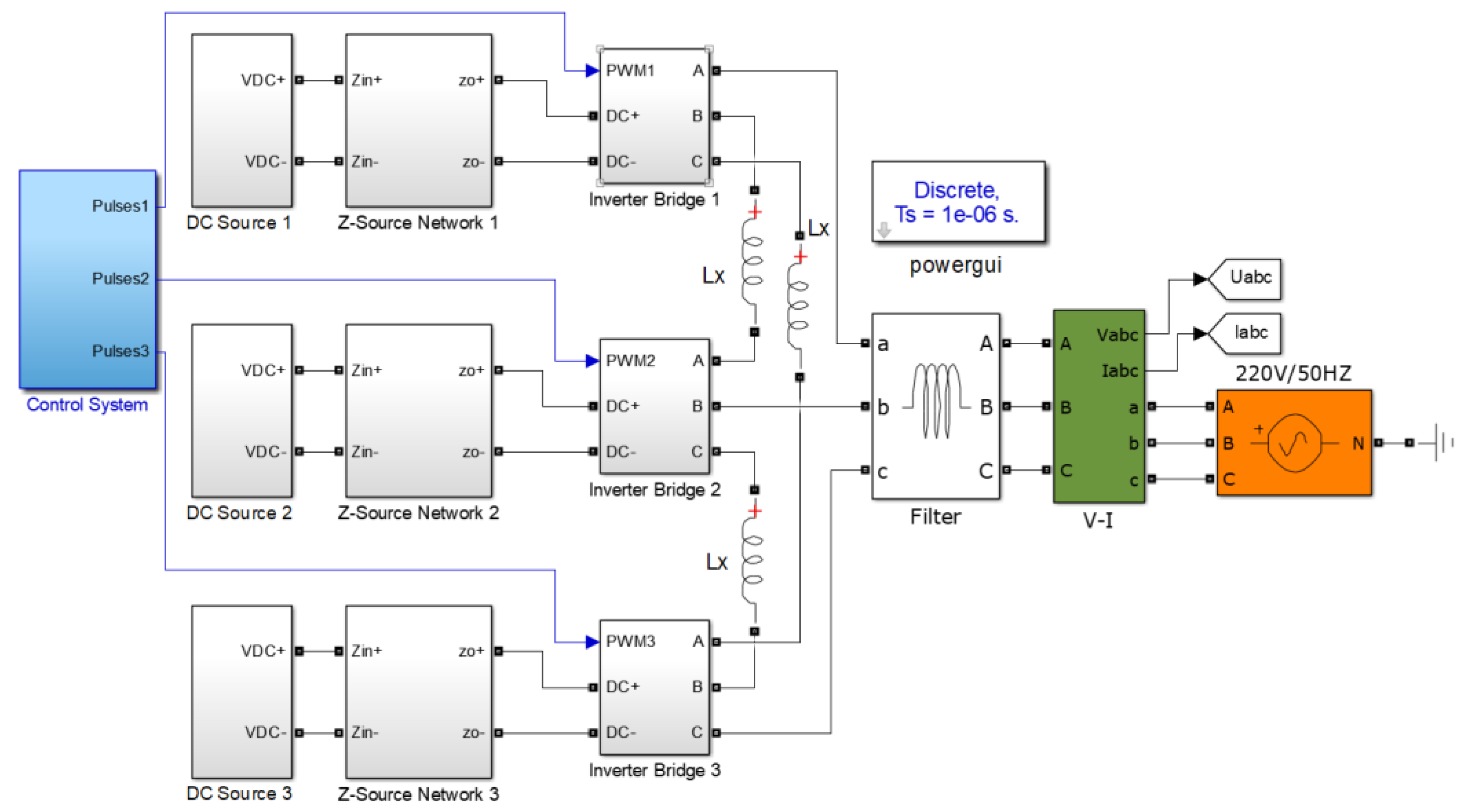
5.1. Experimental Setup

Section 5 builds a LVC-qZSI simulation model in MATLAB 2016/Simulink, and verifies the integration optimization strategy of LVC-qZSI parameters based on GRA-FA. The basic parameters of GRA-FA are as follows: Spatial dimension (3), population size (100), upper limit of iterations (500), step length (0.05). The parameters to be optimized are $L$, $C$, $L_f$, $L_x$, $M$, and $D$, and the values before optimization are shown in

Table 6. Parameters of LVC-qZSI before optimization.

Definition	Value
Z-source network inductance $L$	500 $\mathsf{\mu }\mathrm{H}$
Z-source network capacitance $C$	400 $\mathsf{\mu }\mathrm{F}$
Filter inductance $L_f$	4.00 $\mathrm{mH}$
Cascaded inductance $L_x$	4.00 $\mathrm{mH}$
Voltage of DC source $V_{DC}$	320 $\mathrm{V}$
Modulation index $M$	0.60
Shoot-through duty cycle $D$	0.25
Output frequency $f$	50 $\mathrm{HZ}$
Carrier frequency $f_C$	10 $\mathrm{kHZ}$

. The parameters of each module are set to the same.

5.2. Numerical Results

In Section 3.2, we use GRA to sort six circuit parameters, and the results are shown in Figure 6. In the simulation, we assume that the value range of the preference coefficient $\alpha$ is $\left[0,0.30\right]$, then the corresponding selecting result of optimization variables is $\left[L,C,L_f\right]$. In the process of optimization, with the increase of iterations, the values of optimization variables change constantly. The optimization results from 0 to 500 iterations are shown in

Table 7. Multi-objective optimization results.

Iterations	Optimization Variables	Value
$N=0$	$\left[L,C,L_f\right]$	$\left[500 \mathsf{\mu }\mathrm{H},400 \mathsf{\mu }\mathrm{F},4.00 \mathrm{mH}\right]$
$N=50$	$\left[L,C,L_f\right]$	$\left[308.45 \mathsf{\mu }\mathrm{H},524.90 \mathsf{\mu }\mathrm{F},8.25 \mathrm{mH}\right]$
$N=100$	$\left[L,C,L_f\right]$	$\left[1592.30 \mathsf{\mu }\mathrm{H},863.25 \mathsf{\mu }\mathrm{F},3.80 \mathrm{mH}\right]$
$N=150$	$\left[L,C,L_f\right]$	$\left[1035.60 \mathsf{\mu }\mathrm{H},779.20 \mathsf{\mu }\mathrm{F},5.75 \mathrm{mH}\right]$
$N=200$	$\left[L,C,L_f\right]$	$\left[642.95 \mathsf{\mu }\mathrm{H},887.75 \mathsf{\mu }\mathrm{F},6.95 \mathrm{mH}\right]$
$N=250$	$\left[L,C,L_f\right]$	$\left[954.80 \mathsf{\mu }\mathrm{H},709.15 \mathsf{\mu }\mathrm{F},9.60 \mathrm{mH}\right]$
$N=300$	$\left[L,C,L_f\right]$	$\left[1215.95 \mathsf{\mu }\mathrm{H},1045.80 \mathsf{\mu }\mathrm{F},6.35 \mathrm{mH}\right]$
$N=350$	$\left[L,C,L_f\right]$	$\left[967.15 \mathsf{\mu }\mathrm{H},716.30 \mathsf{\mu }\mathrm{F},15.65 \mathrm{mH}\right]$
$N=400$	$\left[L,C,L_f\right]$	$\left[1056.20 \mathsf{\mu }\mathrm{H},951.55 \mathsf{\mu }\mathrm{F},10.85 \mathrm{mH}\right]$
$N=450$	$\left[L,C,L_f\right]$	$\left[1835.55 \mathsf{\mu }\mathrm{H},1254.75 \mathsf{\mu }\mathrm{F},10.50 \mathrm{mH}\right]$
$N=500$	$\left[L,C,L_f\right]$	$\left[1734.35 \mathsf{\mu }\mathrm{H},1375.90 \mathsf{\mu }\mathrm{F},11.45 \mathrm{mH}\right]$

.

5.3. Results Assessment and Comparison

In Section 5.3, we will evaluate and compare the iterative calculation results of GRA-FA in terms of double frequency voltage ripple ratio and power loss ratio. We set the values of Z-source network inductance, Z-source network capacitance, and filter inductance according to Table 7. Other parameters keep unchanged according to Table 6, and the test time is set to 0.5 s.

Figure 9 shows the voltage waveforms of capacitance $C_1$ when the number of iterations is 0, 100, 200, 300, 400, and 500. It can be seen that with the increase of iterations, the voltage DC component of capacitance $C_1$ basically keeps the constant, while the amplitude of double frequency ripple is decreasing, which is 59.79, 27.82, 18.98, 16.06, 12.08, and 7.55 V. The phase of the double frequency ripple remains unchanged.

At the same time, the voltage waveforms of capacitance $C_1$ are analyzed by Fourier transform in Figure 10a–f. The analysis results indicate that compared with ripples at other frequencies, the ripple at 100 Hz (double frequency) has the highest content. With the increase of iterations, the double frequency ripple content of capacitance voltage is significantly reduced. The total harmonic distortion (THD) of capacitance voltage is 7.69%, 3.42%, 2.38%, 2.02%, 1.54%, and 0.97% (relative to DC), respectively.

Similarly, we calculate the double frequency voltage ripple ratio of capacitance $C_2$ and the power loss ratio, then plot Figure 11 based on the calculation results. On the whole, the double frequency voltage ripple ratio decreases sharply in 0–200 iterations and tends to be stable in 200–500 iterations. Figure 11 shows that after 200 iterations, the value of $R_{C_1}$ decreases from the initial 7.59% to 2.35%, while the value of $R_{C_2}$ decreases from the initial 12.79% to 3.89%. The values of $R_{C_1}$ and $R_{C_2}$ decrease by 69.04% and 69.59%, respectively. Therefore, the optimization of LVC-qZSI parameters based on GRA-FA can effectively reduce the content of the double frequency capacitance voltage ripple. Meanwhile, the calculation speed and effectiveness of the strategy are much higher than the traditional trial and error method. At the same time, Figure 11 shows the dynamic value and change trend of the power loss ratio of LVC-qZSI. It can be seen that with the increase of iterations, the value of $R_{Loss}$ is also decreasing. After 250 iterations, the value of $R_{Loss}$ decreases from 7.26% to 1.93%, a decrease of 73.42%.

In this paper, an integration optimization strategy based on GRA-FA is proposed to obtain optimal LVC-qZSI parameters. The comparison of three performance indexes before and after optimization is shown in

Table 8. Performance comparison before and after optimization.

	${\mathit{R}}_{{\mathit{C}}_1}$ (%)	${\mathit{R}}_{{\mathit{C}}_2}$ (%)	${\mathit{R}}_{\mathit{L}\mathit{o}\mathit{s}\mathit{s}}$ (%)
Before optimization	7.59	12.79	7.26
After optimization	0.95	1.59	1.25

. Table 8 shows that after 500 iterations, the value of $R_{C_1}$ decreases from 7.59% to 0.95%, with a decrease of 87.48%; the value of $R_{C_2}$ decreases from 12.79% to 1.59%, with a decrease of 87.57%; the value of $R_{Loss}$ decreases from 7.26% to 1.25%, with a decrease of 82.78%. It is proved that the optimization effect of the proposed strategy is obvious.

Compare the proposed strategy with other existing strategies. Three different optimization strategies have been investigated: (1) A ripple vector cancellation modulation strategy (RVCMS) based on the thought of ripple vector cancellation [17]; (2) a self-injection APF control strategy for quasi-Z source network ripple suppression [15]; (3) a multi-objective optimization based on MOGA [16].

Table 9. Performance comparison of multiple optimization strategies.

Optimization Strategy	${\mathit{R}}_{{\mathit{C}}_1}$ (%)	${\mathit{R}}_{{\mathit{C}}_2}$ (%)	${\mathit{R}}_{\mathit{L}\mathit{o}\mathit{s}\mathit{s}}$ (%)
RVCMS	2.53	7.75	8.17
APF	0.89	1.34	9.32
MOGA	1.27	1.78	2.41
Proposed	0.95	1.59	1.25

lists the double frequency voltage ripple ratio and the power loss ratio obtained by the proposed strategy and comparison strategies. It can be seen that the values of $R_{C_1}$ optimized by APF, MOGA, and the proposed strategy are 0.89%, 1.27%, and 0.95%, respectively, which are 64.82%, 49.80%, and 62.45% lower than the optimization results of RVCMS. In addition, the values of $R_{C_2}$ optimized by APF, MOGA, and the proposed strategy are 1.34%, 1.78%, and 1.59%, respectively, which are 82.71%, 77.03%, and 79.48% lower than the optimization results of RVCMS. In terms of power loss, the value of $R_{Loss}$ optimized by the proposed strategy is 1.25%, which is 84.70%, 86.59%, and 48.13% lower than the optimization results of RVCMS, APF, and MOGA, respectively. According to the optimization results, the proposed optimization strategy is basically consistent with APF and MOGA in terms of ripple suppression, and all three are superior to RVCMS. In addition, the power loss ratio of the proposed strategy is much lower than the comparison strategies. The simulation results indicate that the proposed optimization strategy can balance ripple suppression and power loss reduction much better.

6. Conclusions

In order to determine reasonable circuit parameters and simplify the multi-objective optimization calculation, we propose an integration optimization strategy of LVC-qZSI parameters based on GRA-FA, and verify the reliability and correctness of the strategy in simulation experiments. The main contributions of this paper are as follows:

(1)

Establish a small signal model of LVC-qZSI, and calculate the double frequency voltage ripples ratios and power loss ratio;

(2)

Summarize the six LVC-qZSI parameters and use GRA to sort them in descending order, then select three main influence factors as optimization variables based on the introduction of preference coefficient;

(3)

Use the information entropy method to assign weights to three objective functions, and construct a multi-objective optimization model of LVC-qZSI parameters;

(4)

Use GRA to improve FA and propose an integration optimization strategy of LVC-qZSI parameters based on GRA-FA;

(5)

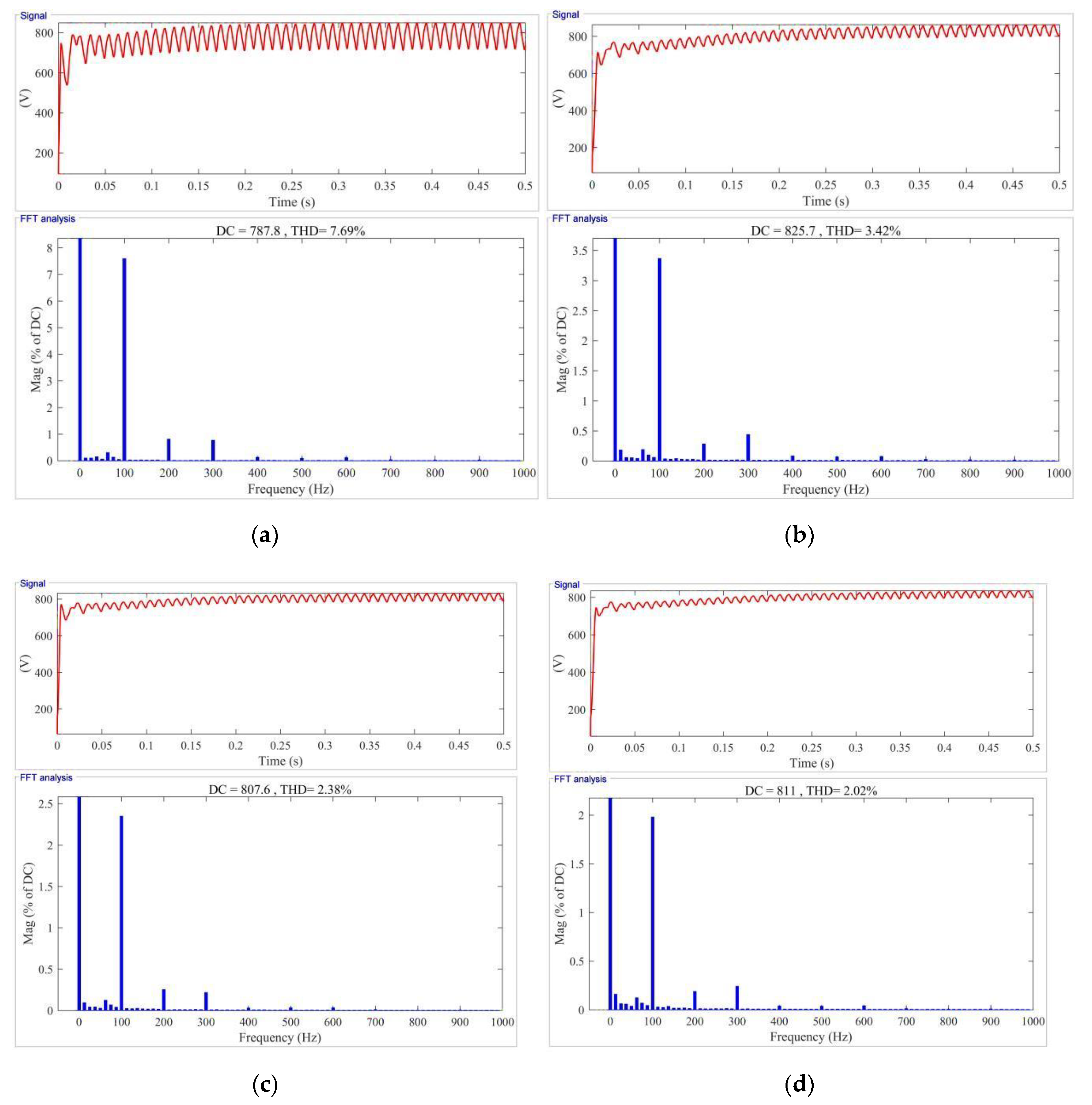
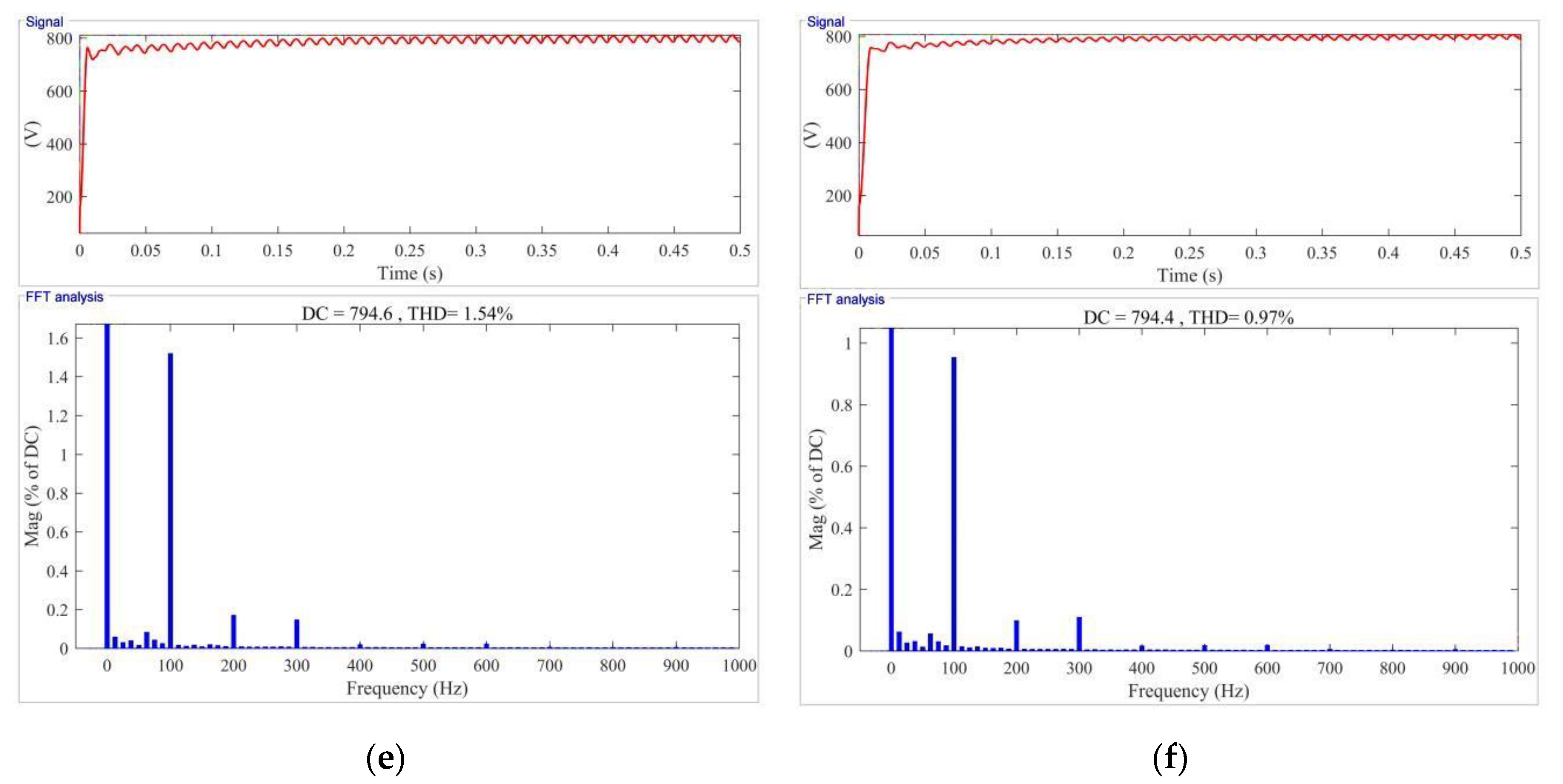
After the iterative calculation of GRA-FA, the values of $R_{C_1}$, $R_{C_2}$, and $R_{Loss}$ are 0.95%, 1.59%, and 1.25%, which are reduced by 87.48%, 87.57%, and 82.78%, respectively. The results indicate that the proposed strategy has excellent optimization ability.

The multi-objective optimization model of LVC-qZSI parameters proposed in this paper uses weight allocation to transform multi-objective optimization into single objective optimization. In the next step, we will solve the multi-objective optimization problem of LVC-qZSI parameters by directly generating the Pareto optimal frontier by extending the firefly algorithm.

References

1. Peng, F.Z. Z-source inverter. IEEE Trans. Ind. Appl. 2003, 39, 504–510. [Google Scholar] [CrossRef]
2. Zhou, Y.; Li, H.; Li, H. A single-phase PV quasi-Z-source inverter with reduced capacitance using modified modulation and double-frequency ripple suppression control. IEEE Trans. Power Electron. 2016, 31, 2166–2173. [Google Scholar] [CrossRef]
3. Khajesalehi, J.; Hamzeh, M.; Sheshyekani, K.; Afjei, E. Modeling and control of quasi Z-source inverters for parallel operation of battery energy storage systems: Application to microgrids. Electr. Power Syst. Res. 2015, 125, 164–173. [Google Scholar] [CrossRef]
4. Belila, A.; Berkouk, E.M.; Benbouzid, M.; Amirat, Y.; Tabbache, B.; Mamoune, A. Control methodology and implementation of a Z-source inverter for a stand-alone photovoltaic-diesel generator-energy storage system microgrid. Electr. Power Syst. Res. 2020, 185, 1–16. [Google Scholar] [CrossRef]
5. Khajesalehi, J.; Sheshyekani, K.; Hamzeh, M.; Afjei, E. High-performance hybrid photovoltaic-battery system based on quasi-Z-source inverter: Application in microgrids. IET Gener. Transm. Distrib. 2015, 9, 895–902. [Google Scholar] [CrossRef]
6. Battiston, A.; Miliani, E.-H.; Pierfederici, S.; Meibody-Tabar, F. Efficiency improvement of a quasi-Z-source inverter-fed permanent-magnet synchronous machine-based electric vehicle. IEEE Trans. Transp. Electrif. 2016, 2, 14–23. [Google Scholar] [CrossRef]
7. Chen, Y.; Jiang, W.; Zheng, Y.; He, G. EMI suppression of high-frequency isolated quasi Z-source inverter based on multi-scroll chaotic PWM modulation. IEEE Access 2019, 7, 146198–146208. [Google Scholar] [CrossRef]
8. Guisso, R.A.; Andrade, A.M.S.S.; Hey, H.L.; Martins, M.L.d.S. Grid-tied single source quasi-Z-source cascaded multilevel inverter for PV applications. Electron. Lett. 2019, 55, 342–343. [Google Scholar] [CrossRef]
9. Hu, S.; Liang, Z.; Fan, D.; He, X. Hybrid ultracapacitor-battery energy storage system based on quasi-Z-source topology and enhanced frequency dividing coordinated control for EV. IEEE Trans. Power Electron. 2016, 31, 7598–7610. [Google Scholar] [CrossRef]
10. Li, Z.; Huang, G.; Zhang, W.; Tang, Y.; Chen, Y. Cascaded three-phase quasi-Z source photovoltaic inverter. In Proceedings of the 2018 8th International Conference on Power and Energy Systems (ICPES), IEEE, Colombo, Sri Lanka, 21–22 December 2018; pp. 6–10. [Google Scholar]
11. Steinbring, M.; Pacas, M. Increasing the efficiency of a single phase Z-source inverter by utilizing SiC-MOSFETS. In Proceedings of the PCIM Europe 2014; International Exhibition and Conference for Power Electronics, Intelligent Motion, Renewable Energy and Energy Management, VDE, Nuremberg, Germany, 20–22 May 2014; pp. 1–7. [Google Scholar]
12. Ozpineci, B.; Tolbert, L.M.; Islam, S.K. Silicon carbide power device characterization for HEVs. In Proceedings of the Power Electronics in Transportation, Auburn Hills, MI, USA, 24–25 October 2002; pp. 93–97. [Google Scholar]
13. Rabkowski, J. Improvement of Z-source inverter properties using advanced PWM methods. In Proceedings of the 2009 13th European Conference on Power Electronics and Applications, Barcelona, Spain, 8–10 September 2009; pp. 1893–1901. [Google Scholar]
14. Sun, D.; Ge, B.; Yan, X.; Abu-Rub, H.; Bi, D.; Peng, F.Z. Impedance design of quasi-Z source network to limit double fundamental frequency voltage and current ripples in single-phase quasi-Z source inverter. In Proceedings of the 2013 IEEE Energy Conversion Congress and Exposition (ECCE), Denver, CO, USA, 15–19 September 2013; pp. 2745–2750. [Google Scholar]
15. Pu, S.; Li, Z.; Chen, Y.; Tang, Y.; Wei, R. A novel ripple self-injection APF for quasi-Z-source inverter. In Proceedings of the 2019 9th International Conference on Power and Energy Systems (ICPES), Perth, Australia, 10–12 December 2019; pp. 1–6. [Google Scholar]
16. Hosseini, S.M.; Beromi, Y.A. A multi-objective optimization for performance improvement of the Z-source active power filter. J. Electr. Eng. 2016, 67, 358–364. [Google Scholar] [CrossRef] [Green Version]
17. Tang, Y.; Li, Z.; Chen, Y.; Wei, R. Ripple vector cancellation modulation strategy for single-phase quasi-Z-source inverter. Energies 2019, 12, 3344. [Google Scholar] [CrossRef] [Green Version]
18. Wei, W.; Hongpeng, L.; Jiawan, Z.; Dianguo, X. Analysis of power losses in Z-source PV grid-connected inverter. In Proceedings of the 8th International Conference on Power Electronics-ECCE Asia, Jeju, Korea, 30 May–3 June 2011; pp. 2588–2592. [Google Scholar]
19. Franke, W.; Mohr, M.; Fuchs, F.W. Comparison of a Z-source inverter and a voltage-source inverter linked with a DC/DC-boost-converter for wind turbines concerning their efficiency and installed semiconductor power. In Proceedings of the 2008 IEEE Power Electronics Specialists Conference (PESC), Rhodes, Greece, 15–19 June 2008; pp. 1814–1820. [Google Scholar]
20. Kumar, A.; Singh, R.K. Power loss calculation of diode assisted cascaded quasi-Z-source converter with CCM and DCM operation. In Proceedings of the 2016 IEEE 6th International Conference on Power Systems (ICPS), New Delhi, India, 4–6 March 2016; pp. 1–6. [Google Scholar]
21. Wang, H.; Wang, W.; Cui, L.; Sun, H.; Zhao, J.; Wang, Y.; Xue, Y. A hybrid multi-objective firefly algorithm for big data optimization. Appl. Soft. Comput. 2018, 69, 806–815. [Google Scholar] [CrossRef]
22. Dac-Khuong, B.; Tuan Ngoc, N.; Tuan Duc, N.; Nguyen-Xuan, H. An artificial neural network (ANN) expert system enhanced with the electromagnetism-based firefly algorithm (EFA) for predicting the energy consumption in buildings. Energy 2020, 190, 1306–1317. [Google Scholar]
23. Bramerdorfer, G.; Zăvoianu, A. Surrogate-based multi-objective optimization of electrical machine designs facilitating tolerance analysis. IEEE Trans. Magn. 2017, 53, 1–11. [Google Scholar] [CrossRef]
24. Zeng, X.; Wu, J.; Wang, D.; Zhu, X.; Long, Y. Assessing Bayesian model averaging uncertainty of groundwater modeling based on information entropy method. J. Hydrol. 2016, 538, 689–704. [Google Scholar] [CrossRef]
Figure 1. Single module topology of the line voltage cascaded quasi-Z-source inverter (LVC-qZSI).
Energies 13 04391 g001
Figure 2. Main circuit topology of LVC-qZSI.
Energies 13 04391 g002
Figure 3. Three-phase current vectors.
Energies 13 04391 g003
Figure 4. Energy flow of LVC-qZSI.
Energies 13 04391 g004
Figure 5. LVC-qZSI circuit system.
Energies 13 04391 g005
Figure 6. Comprehensive correlation degrees of LVC-qZSI parameters.
Energies 13 04391 g006
Figure 7. Grey relation analysis-firefly algorithm (GRA-FA) flowchart.
Energies 13 04391 g007
Figure 8. Integration optimization strategy of LVC-qZSI parameters based on GRA-FA.
Energies 13 04391 g008
Figure 9. Voltage waveforms of Z-source network capacitance C 1 .
Energies 13 04391 g009
Figure 10. Fourier analysis of voltage waveforms. (a) N = 0 ; (b) N = 100 ; (c) N = 200 ; (d) N = 300 ; (e) N = 400 ; (f) N = 500 .
Energies 13 04391 g010aEnergies 13 04391 g010b
Figure 11. Curves of double frequency voltage ripples ratios and power loss ratio.
Energies 13 04391 g011