Function Estimation in Inverse Heat Transfer Problems Based on Parameter Estimation Approach


Zienkiewicz Centre for Computational Engineering, Bay Campus, College of Engineering, Swansea University, Fabian Way, Crymlyn Burrows, Swansea SA18EN, UK
Energies 2020, 13(17), 4410; https://doi.org/10.3390/en13174410
Submission received: 9 July 2020
/
Revised: 21 August 2020
/
Accepted: 24 August 2020
/
Published: 26 August 2020
Abstract
:A new sensitivity analysis scheme is presented based on explicit expressions for sensitivity coefficients to estimate timewise varying heat flux in heat conduction problems over irregular geometries using the transient readings of a single sensor. There is no prior information available on the functional form of the unknown heat flux; hence, the inverse problem is regarded as a function estimation problem and sensitivity and adjoint problems are involved in the solution of the inverse problem to recover the unknown heat flux. However, using the proposed sensitivity analysis scheme, one can compute all sensitivity coefficients explicitly in only one direct problem solution at each iteration without the need for solving the sensitivity and adjoint problems. In other words, the functional form of the unknown heat flux can be numerically estimated by using the parameter estimation approach. In this method, the irregular shape of heat-conducting body is meshed using the boundary-fitted grid generation (elliptic) method. Explicit expressions are given to compute the sensitivity coefficients efficiently and the steepest-descent method is used as the minimization method to minimize the objective function and reach the solution. Three test cases are presented to confirm the accuracy and efficiency of the proposed inverse analysis.
1. Introduction
Direct heat transfer problems are concerned with the determination of temperature distribution in a heat-conducting body from known values for thermo-physical properties, geometrical configuration, boundary conditions, and heat flux. In contract, inverse heat transfer problems (IHTPs) deal with the determination of the thermo-physical properties, the geometrical configuration, the boundary conditions, and the heat flux from the knowledge of the temperature distribution within or on some part of the boundary of the heat-conducting body. Unlike the direct heat transfer problems which are well-posed, the inverse heat transfer problems are ill-posed and inherently unstable and extremely sensitive to measurement errors. Due to the ill-posed nature of IHTPs, these problems are widely regarded as mathematically challenging problems and many methods have been proposed to address the underlying challenges. Over the past decades, the numerical methods for solving the inverse heat transfer problems have received much attention due to the ever-increasing power of computers. Among the numerical methods used to overcome the instabilities in inverse heat transfer problems are the iterative regularization methods. In these gradient-based methods, the inverse problem solution is improved sequentially, and the number of iterations required to obtain a stable solution is set based on the measurement errors using the discrepancy principle [1,2,3].
During the past decades, inverse heat transfer analysis has been extensively used to estimate the constant and variable heat flux using temperature measurement taken at some points inside the heat conducting body or on some part of the boundary of the body. In [4], a three-dimensional inverse heat conduction problem is solved to determine the unknown transient boundary heat flux in an irregular domain using simulated temperature measurements taken at some appropriate locations and times on different parts of the boundary. Then, the least-squares functional is minimized using the conjugate gradient method. In [5], the inverse problem deals with the estimation of the space-dependent heat flux in two-dimensional steady-state heat conduction problems in the presence of variable thermal conductivity. The conjugate gradient method is used as a minimization method to minimize the least-squares objective function. In [6], the inverse problem is concerned with the simultaneous estimation of heat transfer coefficient and heat flux imposed on different parts of the boundary of an eccentric hollow cylinder. The thermal conductivity of the cylinder varies with space and is not considered constant. In [7], an inverse analysis is used to estimate an imposed heat flux on the inner surface of a long cylinder in a transient heat conduction problem using the measured temperature on the outer surface of the cylinder. In [8], a time-dependent heat flux applied at the inner surface of a functionally graded hollow cylinder is estimated via inverse analysis. The simulated temperature measurements are taken within the cylinder and the minimization of the functional is performed by the conjugate gradient method. In [9], an inverse analysis is employed to estimate the unknown base heat flux in an irregular fin made of a material with space-dependent thermal conductivity. The temperature measurements are taken within the fin and the conjugate gradient is used to minimize the objective function. In [10], using an inverse analysis, the heat flux applied on the high-temperature wall of an engine is estimated. The thermal conductivity is a function of temperature and the imposed heat flux is a function of time and position. In [11], the surface heat flux is estimated from two temperature measurements taken inside a finite domain with temperature-dependent thermal properties using a sequential inverse method. In [12], a time-dependent wall heat flux applied on the surface of a solid medium is estimated using an inverse analysis in which the minimization of the functional is performed by the Levenberg-Marquardt method. The temperature measurement data are obtained from thermocouples embedded inside the solid medium.
Inverse problems can be regarded either as a parameter estimation or as a function estimation approach [2]. The parameter estimation approach can be used whenever the unknown quantity can be expressed by a few parameters. For example, the recovery of a constant thermal conductivity can be viewed as a parameter estimation approach. However, if no prior information is available on the functional form of the unknown quantity, then the function estimation approach should be used to estimate the unknown functional form of the unknown quantity. To the best of the author’s knowledge, this study is the first one in which the unknown functional form of a variable heat flux is estimated by the parameter estimation approach through the simultaneous estimation of so many parameters efficiently and accurately.
The function estimation approach to estimate timewise varying surface heat flux, when no a priori information is available on the functional form of the variable heat flux, involves the solution of sensitivity and adjoint problems which require additional mathematical developments and have computational costs equivalent to that of the direct problem. In this study, the inverse problem is formulated based on the parameter estimation approach to solve the function estimation problem of the recovering of the timewise varying heat flux with no a priori information of the functional form of the unknown variable heat flux.
To do so, a two-dimensional transient heat conduction equation subjected to appropriate initial and boundary conditions (with Neumann and Robin conditions at boundaries of a general irregular heat conducting body) is solved using an explicit scheme. Initially, the two-dimensional irregular domain is transformed into a regular computational domain, and all computations needed to solve the direct and inverse problem equations are performed in the regular computational domain. A body-fitted grid generation method (here the elliptic grid generation method) is used to mesh the physical domain, and the finite-difference method, a method chosen for its easy-to-implement feature, is used to approximate the derivatives of the field variable (temperature) at the grid nodes by algebraic expressions. A novel, efficient, accurate, and very easy to implement sensitivity analysis scheme is developed to compute the sensitivity (Jacobian) matrix by employing the chain rule to relate the temperature at the sensor place and the timewise varying wall heat flux applied on the part of the domain boundary. As mentioned above, the inverse analysis using the proposed sensitivity analysis scheme is not involved with the sensitivity and the adjoint equations, thereby reducing the associated development efforts and the computational costs significantly. The main novelty of the proposed sensitivity analysis is that all sensitivity coefficients can be computed efficiently in only one direct problem solution (during the transient solution), with no need for the solution of the sensitivity and adjoint equations (to compute the gradient of the objective function with respect to the variables), irrespective of the number of unknown parameters, which is extremely large in this study. A nonlinear least-square formulation is used to define the objective function and the steepest-descent method with an appropriate stopping criterion specified by the discrepancy principle is employed to minimize the objective function and recover the unknown functional form accurately. Three test cases are presented to reveal the accuracy and efficiency of the employed inverse analysis. In this study, three different measurement errors will be considered. As will be shown, the proposed inverse analysis is not strongly affected by the errors involved in the temperature measurements and the unknown timewise varying heat flux can be recovered with good accuracy.
The inverse analysis for the transient heat conduction problem presented in this study is sufficiently general; that is, it can be used to estimate the timewise varying wall heat flux applied on part of the boundary of a general irregular two-dimensional region (a heat-conducting body) with both Neumann and Robin conditions at the boundaries as long as the general two-dimensional region can be mapped onto a regular computational domain.
2. Governing Equation
The heat-conducting body shown in Figure 1a is made of a material of constant thermal conductivity , density , and specific heat , and is initially at the temperature . For the time , a timewise varying heat flux is applied at the boundary surface . Convective heat transfer is imposed on boundary surfaces with corresponding heat transfer coefficients and surrounding temperatures .
For this problem, the two-dimensional transient heat conduction equation with no heat generation is
The boundary and initial conditions are
where is the time. Since the heat conduction problem is concerned with an irregular body, the irregular shape (the and physical domain) is mapped onto a regular one (the and computational domain). The elliptic grid generation method is used to mesh the domain. Then, the heat conduction equation and its associated boundary and initial conditions can be transformed from the () to the () variables [2,13]. The transformation gives
where and are grid control functions. If , a smooth grid over the physical domain is generated. Thus, Equation (5) becomes
where
are the coefficients obtained from the elliptic grid generation method. The transformed boundary and initial conditions becomes
where is the initial condition rewritten in terms of the variables and . The derivatives appearing in the transformed heat conduction equation, Equation (6) can be discretized in the regular computational domain using the finite-difference method, as follows
where . For the discretization of the boundary condition equations, one-sided forward and one-sided backward relations should be used.
The transformed differential equation, Equation (6), can be approximated by the finite-difference method using the explicit method. Using forward-time-central-space (FTCS) discretization and the relations in Equation (13), we get
where is the time step. Considering stability criterion, Equation (14) can be solved using the time-marching procedure to obtain . In other words, the nodal temperatures at the time level , , can be determined from the knowledge of nodal temperatures at the previous time level , , as follows
3. The Inverse Analysis
3.1. Objective Function
The aim of this study is to estimate the timewise varying heat flux applied at the time and the surface , , using the transient readings of a single sensor placed at the point inside the body. To do so, an inverse analysis is used so that the square of the difference between the estimated temperatures at the sensor place, , computed from the solution of the direct heat conduction problem using the estimated heat flux and the measured temperatures over the time domain is minimized. This can be mathematically expressed as
where . The inverse analysis is used to minimize the following objective function expression:
3.2. Sensitivity Analysis
The inverse problem is concerned with the calculation of the gradient of the objective function J defined by Equation (17) with respect to ,. Thus, we can write
In Equation (18), (, ) are called the sensitivity coefficients and can be explicitly expressed using the chain rule (using the constant thermal conductivity ) as follows
The term in the numerator of Equation (19), , can be obtained by taking the derivative of the solution of Equation (15), , with respect to ,as follows
The term in the denominator of Equation (19),, can be obtained from the boundary condition involving the applied heat flux, Equation (8), as follows
therefore, we get
where the terms , , , , and are computed using the finite-difference expressions associated with the surface .
Therefore, the expression in Equation (19) can be computed by dividing the expression in Equation (20) by the one in Equation (22).
Therefore, the sensitivity coefficients can be computed in only one single direct problem solution (during the transient solution) without the need for solving sensitivity and adjoint problems. The sensitivity matrix can be explicitly written as
3.3. The Steepest-Descent Method
In this study, the steepest-descent optimization method is used to solve the inverse heat transfer problem. In this method, the objective function given by Equation (17) is minimized by searching along the direction of descent using a search step length .
The direction of descent is obtained from the gradient direction , as follows
The search step-length is given as follows [2]
Optimization Algorithm
The following algorithm presents the direct and inverse analysis steps used to estimate the timewise varying heat flux applied at the boundary surface :
- Specify the physical domain, the boundary and initial conditions, and the measured temperatures at the sensor place and the time (), .
- Generate the boundary-fitted grid over the heat conducting body using the elliptic grid generation method.
- Solve the direct problem to obtain the temperature values at the sensor place and the time (), , through solving Equations (6)–(12).
- Using Equation (17), compute the objective function ().
- If value of the objective function obtained in step 4 is less than the specified stopping criterion, the optimization is finished. Otherwise, go to step 6.
- Compute the sensitivity matrix from Equation (25).
- Compute the gradient directions from Equation (18).
- Compute the directions of descent from Equation (27).
- Compute the search step lengths from Equation (28).
- From Equation (26), evaluate the new values for , namely .
- Set the next iteration () and return to step 2.
3.4. Stopping Criterion
Without measurement errors, the inverse problem can be terminated if
where is a small specified number chosen based on obtaining stable and appropriate results. In this study, for the case of no measurement error, . For the temperature measurements with error, the discrepancy principle is used to terminate the iterative procedure. In the discrepancy principle, if the difference between estimated and measured temperatures is of the order of magnitude of the measurement errors, then the solution is assumed to be sufficiently accurate, that is,
where is the standard deviation of the measurement errors and is assumed constant in this study (, , and ). We can obtain the following value for by substituting Equation (30) into Equation (17) (objective function definition)
Then, the iterative procedure is terminated when the following criterion is satisfied
here the measured temperatures containing random errors, , , are generated by adding an error term to the exact temperatures to give
where is a random variable with normal (Gaussian) distribution, zero mean, and unitary standard deviation. Assuming 99% confidence for the measured temperature, lies in the range and it is randomly generated by using MATLAB.
4. Results
Three test cases are presented to investigate the accuracy and efficiency of the proposed sensitivity analysis method to estimate the timewise varying heat flux applied on part of the boundary of a heat conducting body. Initially, it is assumed that the heat flux is known, and the transient heat conduction problem is then solved to estimate the temperature at the sensor place at times (). Then, the estimated temperatures are used as simulated measured ones to recover the initially used heat flux. Three different forms of timewise variation are considered for the heat flux, as follows
- (1)
- A step-function in Test case 1:
- (2)
- A sinusoidal function in Test case 2:
- (3)
- A triangular function in Test case 3:
The heat-conducting body is made of stainless steel (type 304). The numerical values of the coefficients involved in the test cases are listed in Table 1.
The grid size is , the sensor is placed at the node (Figure 2), the initial temperature is , the final time is , and the time step is . Thus, the number of transient readings of the single sensor is . This implies that the number of unknown parameters is . Thus, the parameter estimation approach used so far in the literature is not feasible to estimate this extremely large number of unknown parameters. However, it will be shown that using the proposed sensitivity analysis, the estimation of such a large number of unknown parameters is feasible in an accurate and efficient manner.
In this study, three different measurement errors of are considered. The stopping criteria (Equation (31)) for the test cases with these measurement errors are
Since the size of the Jacobian matrix is , we will deal here with a Jacobian matrix of size . As soon as the nodal temperature at the sensor place is calculated at each time , the Jacobian matrix coefficients can be immediately calculated during the transient solution using the explicit expression for the sensitivity coefficients; that is, during the transient solution of the direct problem, the terms , and , are computed from Equations (20) and (22), respectively, and then the sensitivity coefficients can be obtained from
This means that the proposed sensitivity analysis scheme is very efficient and does not contribute significantly to the computational cost of the solution. If we assume that the computational cost of the expression given by Equation (15) at any node () and time is equal to , then the computational cost of the entire transient heat conduction solution for nodes at the final time is approximately equal to . On the other hand, the computational cost of Equation (23) for a single sensor placed at only one node, , at the final time is approximately equal to . Therefore, the computational cost of the computation of Jacobian matrix at each iteration is of the computational cost of the direct problem solution. In this study, since , the computational cost of the computation of Jacobian matrix is of the computational cost of the direct problem solution.
The initial guesses used for the estimation of the unknown timewise varying heat fluxes in the test cases are as follows:
Initially, the temperature distribution for the heat conducting body used in one of the test cases (Test case 2) is compared to the temperature distribution obtained from the commercial finite element software COMSOL to validate the implementation of the direct problem solution. To do so, the timewise varying heat flux given in Test case 2 () is considered. The grid and the temperature distribution obtained by the explicit solver, Equation (15), using the problem data given in Table 1, a grid size of , and the time step are shown in Figure 3a,b, respectively, and the temperature distribution obtained by the finite element software COMSOL is depicted in Figure 3c. The temperature history of the place of the sensor, , obtained by the explicit solver and the software COMSOL is depicted in Figure 4. Moreover, the temperature distribution at the final time at a given line, here along the nodes , , , obtained by the explicit solver and the software COMSOL is shown in Figure 5. The comparison between the results shows very good agreement, thereby confirming the correct implementation of the explicit solver.
Three different functions (step, sinusoidal, and triangular function) are considered for the timewise variation of the applied heat flux to investigate the inverse analysis presented here. These different functions are selected so that they can reflect the accuracy and efficiency of the inverse analysis as they involve sharp comers and discontinuities, which are the most difficult to be recovered by an inverse analysis [2]. Considering the three different functions, a comparison of the initial (guessed), optimal, and desired heat fluxes is shown in Figure 6a, Figure 7a, Figure 8a (for the case of no measurement error, ), Figure 6c, Figure 7c, Figure 8c (for the measurement error of ), Figure 6e, Figure 7e, Figure 8e (for the measurement error of ), and Figure 6g, Figure 7g, Figure 8g (for the measurement error of ). It can be seen that very accurate results are obtained for both cases of no measurement error and the measurement error, even for functions containing sharp comers and discontinuities.
The convergence histories of the objective function for Test cases 1–3 and cases of no measurement error and the measurement errors of , , and are shown in Figure 6b, Figure 7b, Figure 8b (for the case of no measurement error, ), Figure 6d, Figure 7d, Figure 8d (for the measurement error of ), Figure 6f, Figure 7f, Figure 8f (for the measurement error of ), and Figure 6h, Figure 7h, Figure 8h (for the measurement error of ), respectively. Without the measurement error, a 100% reduction in the objective function and complete recovering of the unknown heat flux are achieved in all test cases, which shows the accuracy of the proposed sensitivity analysis scheme. Moreover, an acceptable recovering of unknown heat flux even in the presence of large measurement errors and a significant reduction in the objective function value implies that the proposed inverse analysis is not strongly affected by the errors involved in the temperature measurements. In addition, in all test cases with and without measurement error, a high convergence rate can be seen and an approximately 99% reduction in the objective function value takes place in the first ten iterations. As can be seen in the figures, the number of required iterations to obtain a stable solution using the discrepancy principle in recovering the unknown heat flux is decreased by increasing the measurement error. The only exception is the case of the measurement error of in Test case 2 in which the number of iterations is 467 (larger than 401 for ). The reason is that the iterative process for the case of the measurement error of could be terminated much sooner because the discrepancy principle, Equation (30), is an approximation expression. The value of the objective function at iteration 314 is 101.007 and the value of the objective function at iteration 467 is 99.999. The objective function is decreased from 101.007 to 99.999 in 154 iterations. In other words, one could terminate the iterative process at iteration 314 instead of iteration 467 to get a stable solution. In the case of the measurement error, some oscillatory behaviors are observed around the exact values due to the ill-posed nature of the inverse heat transfer problem. The details of the results, including the initial and desired values for the variable heat flux, the initial and final values of the objective function, the computation time, the number of iterations, and the percentage of the decrease in the objective function, are given in Table 2 (for cases of no measurement error and the measurement errors of , , and ). As can be seen in Table 2, in spite of large unknown variables (10000 in these test cases) and large final time, (), the short computation time in the test cases confirms that the employed inverse analysis based on the proposed sensitivity analysis is very efficient. The results are obtained by a FORTRAN compiler and computations are run on a PC with Intel Core i5 and 6G RAM.
It can also be seen that in a neighborhood of the estimated heat flux deviates from the exact one and approaches the initial heat flux. One method to overcome this drawback and reduce the effects of the initial heat flux on the solution in the time interval of interest is to consider a final time larger than that of interest. From Equation (18) we can write the gradient of the objective function J with respect to as
By approaching the final time , the elements with zero value in the column vectors of the Jacobian matrix Ja increase and there is only one nonzero element in the last column vector (see Equation (25)) because the Jacobian matrix is a lower-triangular matrix. For example, the gradient of the objective function J with respect to the heat flux at the final time, , is
which is a very small number. Substituting a very small value for into Equation (27), , gives a very small value for . Likewise, substituting a very small number for into Equation (26), , results in , as observed.
5. Conclusions
An explicit sensitivity analysis scheme was developed in this study to estimate the unknown functional form of the timewise varying heat flux applied on part of the boundary of a heat-conducting body subjected to specified initial and boundary conditions through transient readings of a single sensor placed inside the body. There was no prior information available on the functional form of the unknown heat flux. Unlike the function estimation approach which is the widespread approach to address this problem, in this study a parameter estimation approach was used for the first time to estimate the unknown functional form accurately and efficiently through demonstrating three test cases. The transient heat conduction equation was solved using an explicit scheme. Initially, the two-dimensional irregular domain was transformed into a regular computational domain and all computations needed to solve the direct and inverse problem equations were carried out in the regular computational domain. The elliptic grid generation method was used to mesh the physical domain and the finite-difference method was used to approximate the derivatives of the field variable (temperature) at the grid nodes by algebraic ones. A novel, efficient, accurate, and very easy to implement sensitivity analysis scheme was developed by using the chain rule to obtain an explicit relation between the temperature at the sensor place and the timewise varying wall heat flux applied on the part of the domain boundary which allowed for the calculation of the sensitivity coefficients at each time step during the transient solution. Thus, the inverse analysis using the proposed sensitivity analysis scheme is not involved with sensitivity and adjoint equations. The main novelty is that all sensitivity coefficients can be computed efficiently in only one direct problem solution (during the transient solution), without the need for the solution of the sensitivity and adjoint equations (to compute the gradient of the objective function with respect to the variables). The steepest-descent method with an appropriate stopping criterion specified by the discrepancy principle was used to minimize the objective function and recover the unknown functional form accurately. The accuracy and efficiency of the proposed numerical procedure were demonstrated through presenting three test cases.
Funding
This research was supported by funding from the European Union’s Horizon 2020 research and innovation programme under the Marie Skłodowska-Curie grant agreement No 663830.
Conflicts of Interest
The author declares no conflict of interest.
References
- Beck, J.V.; Blackwell, B.; Clair, C.R.S. Inverse Heat Conduction: Ill-Posed Problems; Wiley: Hoboken, NJ, USA, 1985. [Google Scholar]
- Özisik, M.; Orlande, H. Inverse Heat Transfer: Fundamentals and Applications; Taylor & Francis: Abingdon, UK, 2000. [Google Scholar]
- Alifanov, O.M. Inverse Heat Transfer Problems; Springer: Berlin/Heidelberg, Germany, 1994. [Google Scholar]
- Huang, C.H.; Wang, S.P. A three-dimensional inverse heat conduction problem in estimating surface heat flux by conjugate gradient method. Int. J. Heat Mass Transf. 1999, 42, 3387–3403. [Google Scholar] [CrossRef]
- Mohebbi, F.; Evans, B.; Shaw, A.; Sellier, M. An inverse analysis for determination of space-dependent heat flux in heat conduction problems in the presence of variable thermal conductivity. Int. J. Comput. MethodsEng. Sci. Mech. 2019, 20, 229–241. [Google Scholar] [CrossRef]
- Mohebbi, F.; Evans, B. Simultaneous estimation of heat flux and heat transfer coefficient in irregular geometries made of functionally graded materials. Int. J. 2020, 100009. [Google Scholar] [CrossRef]
- Golbahar Haghighi, M.; Malekzadeh, P.; Rahideh, H.; Vaghefi, M. Inverse transient heat conduction problems of a multilayered functionally graded cylinder. Numer. Heat Transf. Part A Appl. 2012, 61, 717–733. [Google Scholar] [CrossRef]
- Chang, W.-J.; Lee, H.-L.; Yang, Y.-C. Estimation of heat flux and thermal stresses in functionally graded hollow circular cylinders. J. Therm. Stresses 2011, 34, 740–755. [Google Scholar] [CrossRef]
- Chen, W.-L.; Chou, H.-M.; Yang, Y.-C. Inverse estimation of the unknown base heat flux in irregular fins made of functionally graded materials. Int. Commun. Heat Mass Transf. 2017, 87, 157–163. [Google Scholar] [CrossRef]
- Zhu, Y.; Liu, B.; Jiang, P.-X.; Fu, T.; Lei, Y. Inverse Heat Conduction Problem for Estimating Heat Flux on a Triangular Wall. J. Thermophys. Heat Transf. 2017, 31, 205–210. [Google Scholar] [CrossRef]
- Zhuo, L.; Yi, F.; Meng, S. An inverse method for the estimation of a long-duration surface heat flux on a finite solid. Int. J. Heat Mass Transf. 2017, 106, 1087–1096. [Google Scholar] [CrossRef]
- Yadav, M.K.; Singh, S.K.; Parwez, A.; Khandekar, S. Inverse models for transient wall heat flux estimation based on single and multi-point temperature measurements. Int. J. Therm. Sci. 2018, 124, 307–317. [Google Scholar] [CrossRef]
- Özişik, M.N.; Orlande, H.R.B.; Colaço, M.J.; Cotta, R.M. Finite Difference Methods in Heat Transfer; CRC Press: Boca Raton, FL, USA, 2017. [Google Scholar]
- Özisik, M. Heat Conduction; John Wiley & Sons: Hoboken, NJ, USA, 1993. [Google Scholar]
Figure 1.
Arbitrarily shaped two dimensional heat-conducting body (physical domain) subjected to a timewise varying heat flux on surface and convective heat transfer on surfaces (a) and the corresponding computational domain (b).
Figure 1.
Arbitrarily shaped two dimensional heat-conducting body (physical domain) subjected to a timewise varying heat flux on surface and convective heat transfer on surfaces (a) and the corresponding computational domain (b).

Figure 2.
The place of the sensor , , used to measure the temperature at time .

Figure 3.
Validation of the direct problem solver using the finite element software COMSOL. The result obtained by using our explicit code (a,b), and the result obtained by using COMSOL (c).
Figure 3.
Validation of the direct problem solver using the finite element software COMSOL. The result obtained by using our explicit code (a,b), and the result obtained by using COMSOL (c).

Figure 4.
Comparison of temperature history at the sensor place, , obtained from the explicit solver and the finite-element software COMSOL. (a) Sensor place; (b) temperature history.
Figure 4.
Comparison of temperature history at the sensor place, , obtained from the explicit solver and the finite-element software COMSOL. (a) Sensor place; (b) temperature history.

Figure 5.
Comparison of temperature at nodes at the final time obtained from the explicit solver and the finite-element software COMSOL. The position of nodes (a) and the temperature comparison (b).
Figure 5.
Comparison of temperature at nodes at the final time obtained from the explicit solver and the finite-element software COMSOL. The position of nodes (a) and the temperature comparison (b).

Figure 6.
Estimation of the timewise varying heat flux using an initial guess and objective function versus iteration number (Test case 1) for cases of no measurement error (a,b) and measurement error of (c,d), (e,f), and (g,h). (a) ; (b) ; (c) ; (d) ; (e) ; (f); (g) ; (h) .
Figure 6.
Estimation of the timewise varying heat flux using an initial guess and objective function versus iteration number (Test case 1) for cases of no measurement error (a,b) and measurement error of (c,d), (e,f), and (g,h). (a) ; (b) ; (c) ; (d) ; (e) ; (f); (g) ; (h) .
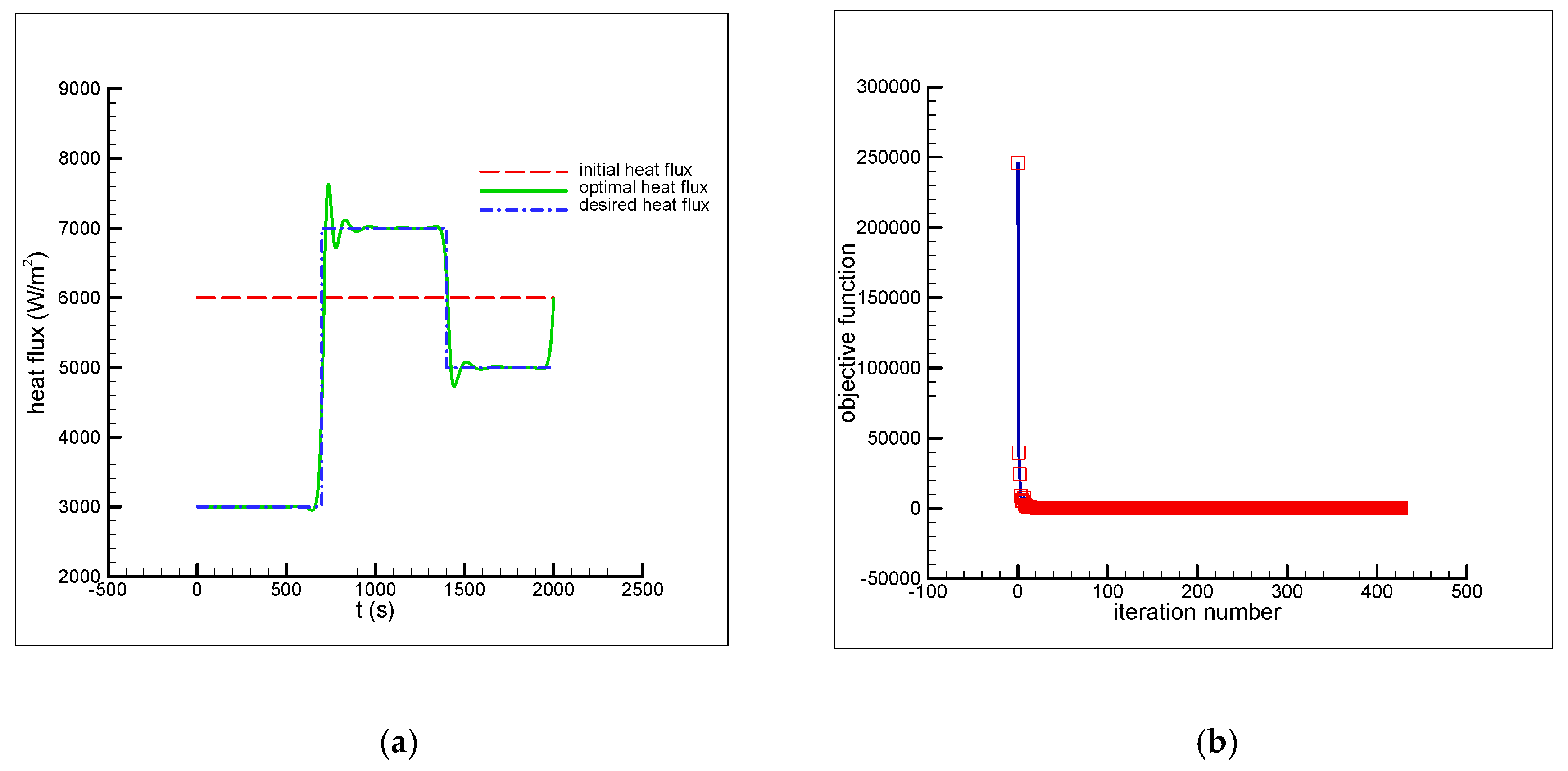

Figure 7.
Estimation of the timewise varying heat flux using an initial guess and objective function versus iteration number (Test case 2) for cases of no measurement error (a,b) and measurement error of (c,d), (e,f), and (g,h). (a) ; (b) ; (c) ; (d) ; (e) ; (f) ; (g) ; (h) .
Figure 7.
Estimation of the timewise varying heat flux using an initial guess and objective function versus iteration number (Test case 2) for cases of no measurement error (a,b) and measurement error of (c,d), (e,f), and (g,h). (a) ; (b) ; (c) ; (d) ; (e) ; (f) ; (g) ; (h) .


Figure 8.
Estimation of the timewise varying heat flux using an initial guess and objective function versus iteration number (Test case 3) for cases of no measurement error (a,b) and measurement error of (c,d), (e,f), and (g,h). (a) ; (b) ; (c); (d) ; (e) ; (f); (g) ; (h) .
Figure 8.
Estimation of the timewise varying heat flux using an initial guess and objective function versus iteration number (Test case 3) for cases of no measurement error (a,b) and measurement error of (c,d), (e,f), and (g,h). (a) ; (b) ; (c); (d) ; (e) ; (f); (g) ; (h) .


Table 1.
Data used for the heat conduction problem (the body is made of stainless steel (type 304)).
Table 1.
Data used for the heat conduction problem (the body is made of stainless steel (type 304)).
| Test Case | ||||||
|---|---|---|---|---|---|---|
| (1) | ||||||
| (2) | ||||||
| (3) |
Table 2.
A summary of results for the estimation of the timewise varying heat flux .
| Test Case | Desired Heat Flux | Initial Heat Flux | Temperature Measurement Error | Initial Value of | Minimum Value of | Reduction in Objective Function & Computation time |
|---|---|---|---|---|---|---|
| (1) | 6000.0 | 245,874.155 | 0.499 | ~100% | ||
| 68 min | ||||||
| (427 iterations) | ||||||
| 246,030.055 | 99.989 | ~100% | ||||
| 56 min | ||||||
| (343 iterations) | ||||||
| 248,653.454 | 2498.254 | 99% | ||||
| 23 min | ||||||
| (137 iterations) | ||||||
| 256,432.253 | 9999.998 | 96.1% | ||||
| 9 min | ||||||
| (58 iterations) | ||||||
| (2) | 4000.0 | 146,727.537 | 0.498 | ~100% | ||
| 64 min | ||||||
| (401 iterations) | ||||||
| 146,826.545 | 99.999 | 99.9% | ||||
| 74 min | ||||||
| (467 iterations) | ||||||
| 149,222.374 | 2499.896 | 98.3% | ||||
| 33 min | ||||||
| (206 iterations) | ||||||
| 156,716.711 | 9999.977 | 93.6% | ||||
| 20 min | ||||||
| (126 iterations) | ||||||
| (3) | 4500.0 | 109,715.236 | 0.419 | 100% | ||
| 16 min | ||||||
| (102 iterations) | ||||||
| 109,841.079 | 99.962 | 99.9% | ||||
| 16 min | ||||||
| (101 iterations) | ||||||
| 112,344.252 | 2496.899 | 97.8% | ||||
| 7 min | ||||||
| (42 iterations) | ||||||
| 119,972.769 | 9997.296 | 91.7% | ||||
| 4 min | ||||||
| (26 iterations) |
© 2020 by the author. Licensee MDPI, Basel, Switzerland. This article is an open access article distributed under the terms and conditions of the Creative Commons Attribution (CC BY) license (http://creativecommons.org/licenses/by/4.0/).
Share and Cite
MDPI and ACS Style
Mohebbi, F. Function Estimation in Inverse Heat Transfer Problems Based on Parameter Estimation Approach. Energies 2020, 13, 4410. https://doi.org/10.3390/en13174410
AMA Style
Mohebbi F. Function Estimation in Inverse Heat Transfer Problems Based on Parameter Estimation Approach. Energies. 2020; 13(17):4410. https://doi.org/10.3390/en13174410
Chicago/Turabian StyleMohebbi, Farzad. 2020. "Function Estimation in Inverse Heat Transfer Problems Based on Parameter Estimation Approach" Energies 13, no. 17: 4410. https://doi.org/10.3390/en13174410
Note that from the first issue of 2016, this journal uses article numbers instead of page numbers. See further details here.