Abstract
It is challenging to apply heat flow through a thermal bridge, which requires the analysis of 2D or 3D heat transfer to building energy simulation (BES). Research on the dynamic analysis of thermal bridges has been underway for many years, but their utilization remains low in BESs. This paper proposes a thermal bridge modeling and a dynamic analysis method that can be easily applied to BESs. The main idea begins with an analogy of the steady-state analysis of thermal bridges. As with steady-state analysis, the proposed method first divides the thermal bridge into a clear wall, where the heat flow is uniform, and the sections that are not the clear wall (the thermal bridge part). For the clear wall part, the method used in existing BESs is applied and analyzed. The thermal bridge part (TB part) is modeled with the linear time-invariant system (LTI system) and the system identification process is performed to find the transfer function. Then, the heat flow is obtained via a linear combination of the two parts. This method is validated by comparing the step, sinusoidal and annual outdoor temperature response of the finite differential method (FDM) simulation. When the thermal bridge was modeled as a third-order model, the root mean square error (RMSE) of annual heat flow with the FDM solution of heat flow through the entire wall was about 0.1 W.
1. Introduction
Globally, governmental policies are focused on reducing carbon emissions. To reduce carbon emissions, energy consumption must be reduced; thus, efforts are being made to reduce energy consumption in all fields, such as industry and transportation. Minimizing energy consumption in buildings is also being studied.
Over the years, research groups focused on building energy have developed various architectural and mechanical techniques to reduce building energy consumption. Developing and evaluating these techniques requires experimental and/or computer simulation methods. Although experimental methods, such as mock-up tests, are important, these methods have limitations in evaluating all cases under various conditions. As a result, the field of BES has consistently evolved, and various building energy analysis and calculation methods have been developed and applied [1,2,3].
The building envelope is the most important part of the BES because it directly protects the building from various external conditions, such as the outdoor temperature [4]. The analysis of the building envelope, which is the physical boundary between the exterior and the interior, is the most basic element of the BES, and many studies have been conducted and applied in this area [5,6,7].
Analysis of the building envelope is done to study the heat transfer phenomena of conduction through the building envelope. Conduction, the mechanism of heat transfer in a solid, is represented by a Fourier equation, which is a differential equation of time and space [8]. Since the BES is numerically calculated for all heat transfer phenomena occurring in a building over one year, if the computing time is too large for one time-step, it is difficult to apply that calculation to the BES [9]. Therefore, analysis of the building envelope is approached while simply assuming a 1D form. In general, the layers constituting the wall can be assumed to have a 1D form, but the thermal bridge is not 1D. A thermal bridge (TB) is defined as the part of the building envelope where the otherwise uniform thermal resistance is significantly changed by full or partial penetration of the building envelope by materials with a different thermal conductivity, and/or a change in thickness of the fabric, and/or a difference between internal and external areas, such as those that occur at wall/floor/ceiling junctions [10]. As can be seen from the definition of TB, TB is difficult to understand with a 1D form because of the complexity of its materials and geometry. On the other hand, a significant part of heat losses in a building can be due to TBs [9]. In some buildings up to 50% of the elevation area includes 3D envelope structural details [11]. It is investigated that the inclusion of thermal bridges increases the annual space heating energy demand by 38–42% and decreases the annual space cooling energy demand by 8–26% [12]. The heat flow through the TB in the building heat balance cannot be ignored, especially if the building is highly insulated [13]. Furthermore, because of the thermal inertia of the TB, the analysis should be performed under dynamic condition in order to accurately analyze the heat flow through the TB [14]. Therefore, the dynamic analysis of TB is a complex multidimensional problem but remains necessary in BES.
Most BES programs, such as EnergyPlus [15] or TRNSYS [16], assume that the heat flow though the building envelope is a uniform heat flow in 1D. In the 1D analysis platform, the heat flow through the TB is ignored because the heat flow, which requires multidimensional analysis, cannot be calculated. On the other hand, there are many thermal fields calculation software capable of multidimensional analysis. Some examples of software mainly used in the building analysis sector include THERM [17], PHYSIBEL [18] and WUFI [19]. THERM is 2D conduction heat transfer analysis program based on the finite element method (FEM), which can model the complicated geometries of building products. THERM can calculate the temperature distribution and heat flow under a steady-state condition, which is related to condensation, moisture damage, and structural integrity. Dynamic analysis and 3D analysis cannot be performed. PHYSIBEL is a software environment for thermal analysis of 2D/3D building components, both steady-state and transient, based on the finite difference method (FDM). In the PHYSIBEL software environment, TRISCO is a program for steady-state thermal simulation and VOLTRA is a program for the dynamic simulation of 3D building components [20,21]. These programs focus solely on the TB analysis itself and are difficult to integrate with BES. WUFI is a hygrothermal simulation program based on the finite volume method (FVM). One of the capabilities of WUFI is that it has integrated modules for dynamic analysis of 3D bodies that can analyze TBs. However, since this program directly applies 3D modeling and analysis of TBs to BES, it takes a lot of time to simulate TBs [12]. To solve this problem in BES, the steady-state analysis results of the TB, which are relatively easy to calculate, are simply added at each time-step in the dynamic analysis. This method is inaccurate because it cannot reflect the time delay and decrement effects caused by the thermal inertia of the TB [9]. Alternatively, a method for reconstructing the building envelope, including the TB, into an equivalent wall and analyzing both in 1D has been proposed. This idea leads to the concept of the “thermally equivalent wall”, a simple structure that has the same type of dynamic thermal behavior as a more complex structure and may be substituted for complex structure in building a design energy simulation [22]. Various methods for constructing an equivalent wall have been studied, and most of the research on TB dynamic analysis in the BES has focused on this method [22,23,24,25]. This powerful method is applicable to the BES program while accurately reflecting the thermal behavior of an unsteady state of the TB, but it is not often used because of its complexity. The parameters supplied by the equivalent wall methods can be directly introduced via the interface of the simulation programs without modification of the source code or of the generated files [9]. However, it is not easy to replace the existing complete source code. In addition, if building engineers want to evaluate and strengthen the thermal performance of the building envelop, it is necessary to determine whether to strengthen the insulation of the clear wall or to supplement TB details, such as the use of thermal breakers [26]. In this case, the amount of heat flow through the clear wall (the clear wall is a part of the wall that is not interrupted by the details [24]. It is a part where heat flow is uniform and can be analyzed in 1D) and the TB part should be divided and simulated in the BES.
The aim of this study is to develop a thermal bridge modeling and a dynamic analysis method that can be efficiently applied to the 1D platform BES program. The modeling and analysis method should be simple and take less time to simulate, and it should be possible to convert 3D analysis into 1D analysis. The scope of the study is to calculate only the total heat flow into the room through the TB rather than calculating all the indoor surface temperatures of the TB according to the outdoor temperature. The proposed TB modeling and dynamic analysis method proceeds by adding the additional analysis model separately from the clear wall analysis code used in the existing BES program. As a result, it is possible to analyze the heat flow through the clear wall and the TB part, separately. The main idea comes from an analogy of steady-state thermal bridge analysis and system identification. Similar to the steady-state analysis of the TB, even under dynamic condition, the heat flow through the TB is divided into heat flow through the clear wall and heat flow through the TB part. This is because heat flow through the clear wall can already be analyzed in the BES program. The remaining part, the TB part, is assumed to be a linear time-invariant system (LTI system) and modeled using a system identification method, which is a data-driven method. The input and output data required are obtained through dynamic analysis for several days using FDM software. The proposed method is verified by comparing the heat flow obtained while applying the proposed method to a specific TB and the heat flow computed by applying the FDM method. The annual heat flow simulated by applying the proposed method was compared with that of existing methods.
2. Thermal Bridge Modeling and Analysis Methods
Several approaches have been applied to analyze the TB. TB modeling and analysis starts by analyzing the conductive heat transfer through the wall. In conduction, the total heat flow rate can be obtained from the temperature gradient, which is Fourier’s first law.
where is the heat flux (W/m2), is the thermal conductivity (W/mK), and is the temperature (K).
The temperature can be obtained for the governing equation, which is called the Fourier’s second law or heat diffusion Equation (2).
where is the temperature (K), is the time (s) and is the thermal diffusivity (m2/s).
Unfortunately, it is difficult to obtain an analytical solution, such as the TB, from Equations (1) and (2) with complex geometry. Instead of an analytical solution, a numerical solution can be obtained via FDM, FVM, FEM or the boundary element method (BEM) [27]. Although a numerical solution can be obtained, it is complicated and time-consuming to solve it and is limited to the BES, which is mainly simulated for one year [9].
Under the theoretical background of TB modeling and analysis, various thermal bridge modeling and analysis methods have been studied. Several papers summarize TB modeling and analysis methods [9,28,29]. The most common method is to ignore the TB and analyze only the clear wall (neglecting the thermal bridge). The method is used because it is challenging to perform a dynamic analysis of TB. Another approach is to analyze the clear wall with a dynamic condition and analyze the TB with a steady-state condition [30]. This method is useful because the BES is performed while reflecting the thermal bridge analysis, but it is inaccurate because it does not reflect the heat capacity. The heat diffusion equation is a partial differential equation(PDE), but there is a method to create and analyze a state-space model by converting a PDE to an ordinary differential equation (ODE) using finite difference spatial discretization [31]. As a result of its greater number of ODEs, a model reduction process is required to apply this state-space model method to the BES. Most of the models for application to the BES, which is a 1D analysis platform, have been studied as a 1D equivalent wall (equivalent wall method) [9]. The method for constructing an equivalent wall can be divided into several methods: the structure factors method [22], the matrix of transfer functions method [23], the one harmonic method [24], and the identification method [25]. Various modeling methods and analysis methods exist and are applicable to the BES in various ways depending on the model’s complexity, accuracy, and analytical convenience. Indeed, there are few cases where a building is analyzed by applying it to a BES, possibly because the models that have been researched are not simple enough or because the developers or users are unfamiliar with a BES. There is a need for a thermal bridge analysis model that is simple and easy to understand and can utilize existing source code for clear wall analysis. Therefore, in this paper, a thermal bridge modeling and dynamic analysis method is proposed in a similar way to the relatively well-known steady-state TB analysis method.
3. Methodology
3.1. Analogy of Steady-State Thermal Bridge Analysis
The steady-state TB analysis is used to calculate the linear thermal transmittance () or the point thermal transmittance () by performing a numerical simulation (the detailed calculation method is found in ISO 10211 [10]). Thermal transmittance is a concept similar to the U-value of the clear wall, which is a physical quantification of how well heat can flow through a TB.
The heat flow rate through a wall between two different environments with two different temperatures can be calculated by Equation (3) [10]:
where is the heat flow rate from 1 to a thermally connected 2 (W), is the thermal coupling coefficient in a 3D calculation (W/K), is the temperature of 1 (K) and is the temperature of 2 (K).
The thermal coupling coefficient is divided by the following three terms:
The detailed description can be found in [10]. The concept of calculating the heat flow rate in a steady state is a linear summation or linear combination of . In other words, the thermal coupling coefficient consists of the heat flow through the clear wall (), the linear thermal bridge part (), and the point thermal bridge part (), each of which has an independent relationship that does not affect the others. In practice, the heat flow through each part affects the other parts, but for convenience, a linear calculation formula is created.
For simplicity, assuming that there is only one linear thermal bridge part and no point thermal bridge part in the wall for the 2D calculation, the linear thermal transmittance () is determined by Equation (5):
where is the thermal coupling coefficient obtained from a 2D calculation using numerical analysis methods, such as FDM, FVM or FEM. is the thermal transmittance of the 1D component and is the length over which the value applies.
The concept for obtaining the linear thermal transmittance becomes clear when Equation (5) is multiplied by the temperature difference. The heat flow through the entire wall minus the heat flow through the clear wall is considered as the heat flow through the linear thermal bridge part. Here, the heat flow through the entire wall is obtained by numerical analysis, and the heat flow through the clear wall is obtained using the existing method (simple hand calculations).
The main idea of TB modeling and the dynamic analysis method in this paper comes from the concept of steady-state TB analysis (Figure 1). Like steady-state analysis, in the dynamic analysis, the heat flow through the TB part is also considered to exclude the heat flow through the clear wall from the heat flow through the entire wall. The only difference is that in steady-state analysis, the heat flow value is a single value, but in dynamic analysis, the heat flow value is a time series value. The method for obtaining the heat flow through the entire wall and the clear wall uses numerical analysis and the existing method in the same way as in the steady-state analysis. When obtaining the heat flow through the entire wall using numerical analysis, the outdoor temperature (which is a boundary condition) is taken as a time-invariant (constant) value in the steady-state and as a time-variant value in the dynamic analysis. The existing method for obtaining the heat flow through the clear wall is a calculation method using the U-value in the steady-state and a method such as the conduction transfer function (CTF) in the BES [32] in the dynamic analysis. Lastly, for steady-state analysis, the factor (which can be the performance indicator for the TB in a steady-state condition) representing heat flow though the TB part is expressed as the linear thermal transmittance, which is a value corresponding to the U-value of heat flow through the clear wall. Likewise, in dynamic analysis, the factor representing heat flow through the TB part should be in a format similar to CTF, a function related to heat flow through the clear wall. Therefore, the TB model for dynamic analysis is a function that can express heat flow through the TB part. Figure 1 shows the analogy of a steady-state TB analysis.
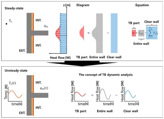
Figure 1.
Concept for the analogy of a steady-state thermal bridge (TB) analysis. is the outdoor temperature and is the heat flow into the room.
To proceed with this proposed method, it is first necessary to clearly disaggregate the range of the clear wall and TB part. In steady-state analysis, the dimension system described in ISO 14683 [33] should be determined for calculating the linear thermal transmittance. This is done to determine the value of in Equation (5). The dimension system is not equivalent to the geometric dimension of the actual TB and is only related to the range that can be analyzed in 1D according to the rules. Although the amount of heat flow through the entire wall is the same, the ratio of heat flow through the clear wall and the TB part is different depending on the dimension system. The linear thermal transmittance varies depending on the dimension system [33], which only involves setting and analyzing the range of the clear wall. Similarly, in dynamic analysis, the dimension system can also be applied. The heat flow through the entire wall does not depend on the dimension system, but the function of the TB part can be different, as the value of the linear thermal transmittance varies depending on the dimension system in a steady state. Therefore, in order to analyze the heat flow through the TB part in addition to the heat flow already calculated in BES, the dimension system should be determined according to the analysis range of the clear wall (wall area) in BES.
3.2. Linear Time Invariant System for the Thermal Bridge Part and System Order
To complete the concept obtained by the analogy of a steady-state thermal bridge analysis, it is necessary to find the function of the TB part. The function of the TB part expresses the heat flow into the room through the TB part according to the outdoor temperature. Since the theoretical background is rendered via Equations (1) and (2), the TB part can be defined by the linear time-invariant system (LTI system), and this relationship is expressed in the general formula below:
where is the heat flow rate into the room through the TB part (the output of the system), is the outdoor temperature (the input), and are the coefficient of the LTI system.
This LTI system can also be derived with a thermal network model, a method of wall analysis (Appendix A). For the right term of Equation (6), the derivative term of the outdoor temperature is not related to the LTI system, and only the constant multiple of the outdoor temperature affects the LTI system:
In the state-space model, the ODEs obtained using finite difference spatial discretization can also be expressed via Equation (7), but the system order, which is the highest order of the linear differential equation, becomes very large. The higher the system order is, the higher the accuracy of the model muse be. This process becomes complicated and time-consuming, so it is necessary to choose the system order to simplify the model.
3.3. Thermal Bridge Transfer Function and System Identification
The function of the TB part mentioned above can be expressed as a transfer function related to the input and output relationship. The transfer function of a linear time-invariant differential equation system is defined as the ratio of the Laplace transform of the output to the Laplace transform of the input under the assumption that all initial conditions are zero [34]. CTF also originates from the transfer function, and wall conduction analysis using the transfer function has been studied and widely used [35]. Therefore, the model for the TB part can be easily applied to the BES by expressing it as a transfer function. Using Equation (7), the transfer function of TB part (TBTF) is as shown in Equation (8).
where is the Laplace transformation and is the complex variable.
To estimate the coefficients () in Equation (8), the system identification process can be applied. System identification (SI) is defined as the exercise of developing a mathematical relationship (model) between the cause (inputs) and the effects (outputs) of a system(process) based on observed or measured data [36]. There are several methods for the system identification, but all require input and output data of the system. Input data for this system can be generated as a boundary condition for the numerical analysis of TB, and the output data can be obtained as a result of numerical analysis in a dynamic simulation (Figure 2). Importantly, since the LTI system is set for the TB part, the heat flow into the room corresponding to the output data excludes the heat flow through the clear wall from the heat flow through the entire wall, which is similar to steady-state analysis. Since the proposed method is configured to divide the entire wall into a clear wall and a TB part to be linearly coupled, heat flow through the clear wall part and the TB part can be calculated separately. The input data correspond to the boundary condition in dynamic simulation, so it can be arbitrarily established by the user who simulates it. The input data for the SI process can be arbitrary time series data, but step input is used as the input data in this study because various characteristics of the system can be identified through a step-response.
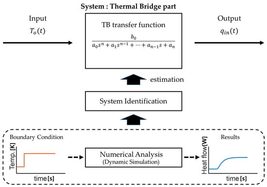
Figure 2.
The strategy of the system identification for the TB part. System identification is used to estimate the parameters of the TB transfer function. Input/output data required for system identification are obtained through numerical analysis (dynamic simulation).
3.4. Procedure
The proposed method involves disaggregating the thermal bridge into the clear wall and TB parts, similar to the steady-state TB analysis method, and linearly combining each thermal characteristic. For the clear wall, the existing method of dynamic analysis is applied, and for the TB part, the transfer function using the system identification process is applied. The modeling procedure can be summarized as follows:
- Step 1: Disaggregation stageDetermine the dimensional system.
- Step 2: Dynamic simulation stagePerform the dynamic simulation of the entire wall and the clear wall.
- Step 3: Model construction stageChoose the LTI system order of the TB part and construct the TBTF.
- Step 4: System identification stageObtain the parameter of TBTF using the system identification process.
4. Explanatory Example
To apply and validate this methodology, a simple thermal bridge model is analyzed according to the procedure of the proposed method. The target wall is selected as the wall of a general residential building, the same as the wall suggested in a previous paper [37]. The model geometry is shown in Figure 3a, and the material dimensions and thermal properties are shown in Table 1.
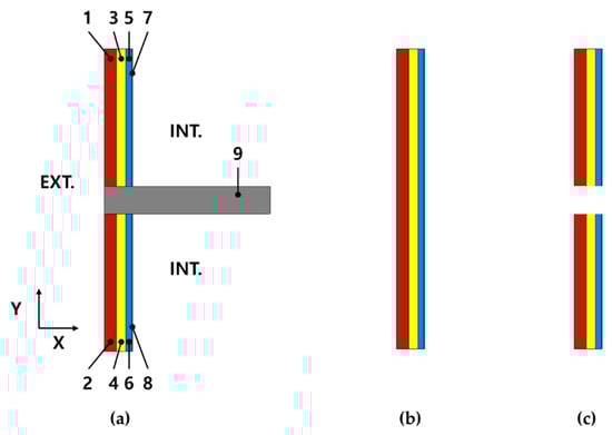
Figure 3.
Geometry of model: (a) the entire wall (1–9 is the material number in Table 1); (b) the clear wall (external dimension system); (c) the clear wall (internal dimension system).

Table 1.
The material dimensions and thermal properties.
Before the analysis, a steady-state simulation is performed to determine the state of the target wall and compare it with the dynamic analysis results. Commercial software, TRISCO [20], is used for the process and the results are shown in Table 2. The steady-state performance indicators in Table 2 differ slightly depending on the mesh grid size of the numerical simulation.
Table 2.
Steady-state analysis results (grid size: 20 mm).
4.1. Disaggregation Stage: Step 1
As mentioned in Section 3.4, the first step is to disaggregate the entire wall into the clear wall and TB part. This is a separation process for a linear combination by calculating the heat flow through each part, and the heat flow through each part varies according to the dimension system related to the analysis range of the clear wall in BES. Figure 4 conceptually illustrates the heat flow in a steady state according to the dimension system. Therefore, the meaning of disaggregation is to determine the dimension system, which affects the geometry of the clear wall model in the next step (Figure 3b,c).
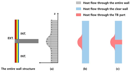
Figure 4.
The heat flow in steady-state analysis according to the dimension system: (a) the entire wall; (b) external dimension system; (c) internal dimension system.
In this case study, the external dimension system is determined, and the clear wall is disaggregated into the geometry as shown in Figure 3b.
4.2. Dynamic Simulation for System Identification: Step 2
The input and the output data for the SI of the TB part are obtained by performing a dynamic simulation, which involves a numerical analysis. The commercial software, VOLTRA [21], is used for this purpose. This software is capable of 3D dynamic analysis; the FDM method is also applied.
The input data are the outdoor temperature (), and the output data are the heat flow into the room through the TB part (). Notably, the heat flow through the TB part corresponds to the output. The dynamic simulation of a TB usually yields in the value of the heat flow through the entire wall, including the TB part. Since the entire wall is divided into the clear wall and the TB part, the heat flow through the clear wall must be excluded from the heat flow through the entire wall to obtain the heat flow through the TB part. In a steady state, the heat flow value through the clear wall can be easily calculated using the U-value, but in an unsteady-state, the time series heat flow data cannot be easily calculated. Therefore, it is necessary to perform additional simulations to obtain the output for the same input data by modeling only the clear wall. The method for obtaining the heat flow through the TB part is conceptually illustrated in Figure 5.
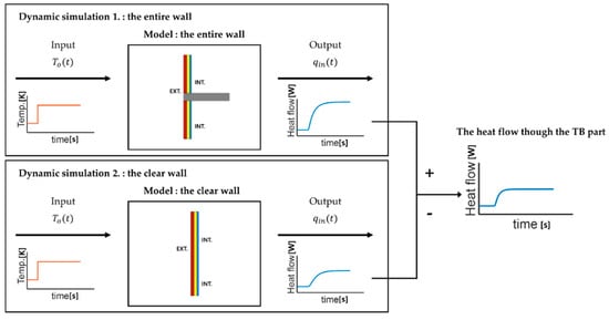
Figure 5.
The method for obtaining the heat flow through the TB part. The heat flow through the TB part is calculated by subtracting the heat flow through the clear wall (dynamic simulation 2) from the heat flow through the entire wall (dynamic simulation 1). is the outdoor temperature and is the heat flow into the room.
The outdoor temperature corresponding to the input data (or boundary condition) is given as a step function from 0 °C to 20 °C after one day and the indoor temperature and initial temperature of all structures are 0 °C. The simulation duration was set to 20 days, which is a sufficient time to reach a steady state. For accuracy, the simulation time step is set as 60 s (Table 3).
Table 3.
Simulation configuration.
4.3. Model Construction and Transfer Function: Step 3
The system model is constructed by assuming that the TB part is an LTI system. At this time, the system order should be chosen to produce a simple TBTF. Since the highest power of in the denominator of the transfer function is the system order, choosing the system order is the same as determining the form of the TBTF. In this case study, the first to fourth order are chosen without specifying the system order. The most accurate and efficient system model can then be selected by comparing the four case models estimated through the system identification process with the FDM model. It should be noted that the number of zeros corresponding to the numerator is 0. Therefore, to obtain the TBRF, the number of parameters to be estimated is the system order plus one.
4.4. System Identification: Step 4
System identification is performed with the outdoor temperature (input) and heat flow into the room through the TB part (output), which are the results of the dynamic simulation in Step 2. Here, we use the model form constructed in step 3.
There are several methods and tools for system identification. In this example, system identification is performed using MATLAB, and the main function is “tfest”. The algorithm of tfest is the Instrument Variable (IV) method for parameter initialization, and the nonlinear least-squares search method is used to update the parameters [38]. Although the parameters are estimated using the system identification tool, TBTF can be found by simple curve fitting. Since the input data are constant as a step function, and the form of the model to be estimated is determined, it is possible to curve fit the output with the solution formed by the differential equation.
5. Results and Validation
5.1. Dynamic Simulation Results and System Identification Results
The result of the dynamic simulation is shown in Figure 6. The data for system identification of the TB part include the outdoor temperature as input data and the heat flow into the room through the TB part as the output data. All data are time series data, with 28,800 values for 1,728,000 s (20 days) at 60 s intervals. To verify the result of the dynamic simulation for system identification, this result is compared with the steady-state result. Since the input data of the dynamic simulation are made constant with the step function, the final heat flow value of the dynamic simulation must be similar to the steady-state result. The comparison results are shown in Table 4. This simulation is considered valid because the steady state errors for all the results of the entire wall, clear wall and the TB part are very small (under 0.001%).
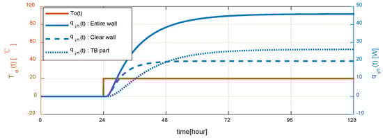
Figure 6.
Dynamic simulation results for system identification of the TB part. is the outdoor temperature and is the heat flow into the room.
Table 4.
Final values of dynamic simulation and the time to reach 99.99% of the steady-state value.
One of the considerations when performing a dynamic simulation for system identification is the simulation duration. The longer the simulation duration is set, the greater the amount of input and output data when the same time step is applied. The system can be estimated more accurately using a large amount of input and output data, but this is inefficient because data that have reached a near steady state and have changed little are meaningless. Therefore, it is recommended to run the simulation for 10 days, which is twice the time needed to reach 99.99% of the steady-state value; at least 5 days should be simulated.
Table 5 shows the results of the system identification. Here, the model accuracy increases as the system order increases. For the fourth-order system model, the FPE and MSE show accuracy with a value of 0 to the fourth decimal place.
Table 5.
System identification results.
5.2. Validation of the System Identification
The validation of the SI is the most important step to ensure that the heat flow into the room through the entire wall including the TB part, which is the final result of the proposed method, is accurate. This is because the clear wall is calculated using the existing verified method, while only the model for the TB part is estimated by the SI. To validate of the models, the heat flow into the room according to three inputs (step input, sinusoidal input and annual outdoor temperature) is compared with the heat flow calculated using the FDM model. The three inputs are shown in Table 6 and Figure 7. The step input is the same as the input for the SI. Since the outdoor temperature changes mainly with each day, the sinusoidal input is set to a 24 h periodic function with an amplitude of 20 °C. Lastly, since the accuracy of each model according to the step input cannot be guaranteed when the actual outdoor temperature is used as the input, the annual outdoor temperature from the weather data in Seoul, South Korea, which is applied in the BES, is used for validation. As shown in Figure 7, this outdoor temperature data cover one year, and the time step is 1 h, which yields 8760 data (max.: 31.3 °C; min.: −10.6 °C).
Table 6.
Inputs for validation of the system identification.
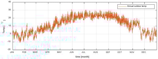
Figure 7.
Annual outdoor temperature input.
The heat flow calculated using the FDM model is simulated using VOLTRA, a previously used commercial program. It is also assumed that the heat flow data obtained by simulation using the FDM model are actual values. The heat flow using all the models estimated above (from the 1st-order to the 4th-order model) is simulated using MATLAB. “lsim”, a function in MATLAB, is used to simulate the time response of the dynamic system to arbitrary inputs for the estimated model [38].
Comparison graphs for the step response and sinusoidal response are shown in Figure 8 and Figure 9. The rest of the models, except for the first-order model, are almost identical to the FDM simulation results. Since the first-order model is the simplest model for the TB part, it can be easily produced; however, its accuracy is lower than that of other models. On the other hand, it is difficult to distinguish the fourth-order model from the results of the FDM model in the graph. In the sinusoidal response comparison, the amplitude and time shift of the fourth-order model are also almost the same for the FDM (Table 7). The third-order model also shows very accurate results.
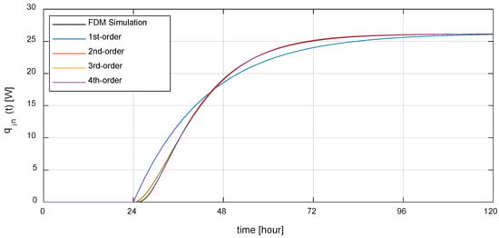
Figure 8.
Step response of the models.
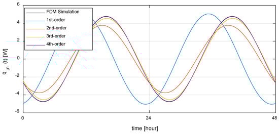
Figure 9.
Sinusoidal response of the models.
Table 7.
Amplitude and time shift comparison with the FDM sinusoidal response.
Figure 10 presents a graph comparing the simulation results of each model for one year. The results of FDM and all other estimated models are almost the same, so it is difficult to distinguish each result with a graph for one year. For a more detailed illustration, the results for a specific period (6 days from 15 August to 20 August in summer) are shown in Figure 11. The first-order model has apparent differences from the other estimated models. In the second-order model, a distinguishable error occurs, but in the third-order and fourth-order models, there is almost no difference from the FDM model results. Figure 12 shows the graph of each model error over time for one year, and Table 8 shows the root mean square error (RMSE) of each model. The most accurate model is the fourth-order model, whose RMSE value is 0.0895 W. The accuracy increases as the system order increases, but the complexity of the model also increases. Considering that the heat flow through the entire wall is 45.8376 W under steady-state conditions (when the indoor and outdoor temperature difference ) and −38 W–10 W in the annual simulation, the RMSE of the third-order model, which is only 0.1007 W, remains accurate, even if the TB part is estimated as a third-order model. Indeed, even the RMSE value of the first-order model, the most inaccurate model, is only 0.6920 W. Therefore, all estimated models can be used for BES. In addition, considering the model complexity and the accuracy of the results, it is recommended to estimate the TB part as a third-order model. The simplest modeled first-order model is slightly inaccurate but remains sufficient for BES with TB. Therefore, the proposed method is validated.

Figure 10.
System response for the annual outdoor temperature.

Figure 11.
System response for the annual outdoor temperature (Summer).
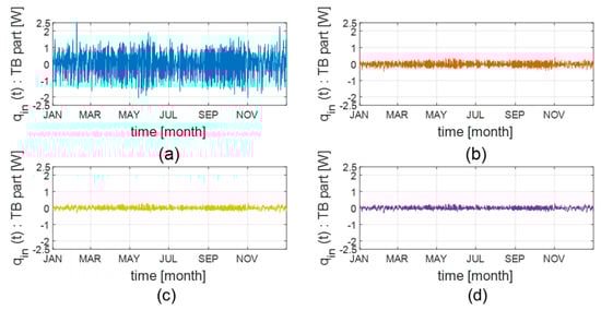
Figure 12.
Residual of the heat flow rate: (a) First-Order model; (b) Second-Order model; (c) Third-Order model; (d) Fourth-Order model.
Table 8.
System response RMSE of each model for the annual outdoor temperature.
6. Comparison and Discussion
Thus far, the modeling of the TB part using the proposed method has been described and discussed. This model will now be described with a focus on the heat flow through entire wall, including the TB part. In the BES, it is also important to analyze only the TB part, albeit focusing more on the heat flow into the room through the entire wall for various purposes, such as calculating the indoor temperature or controlling the heating and cooling system. Therefore, the annual heat flow into the room through the entire wall is calculated using the proposed method and then compared to the results of the calculations using other models. The other models are defined as follows.
- FDM simulation: A model defined as a true value in this comparison simulated by the FDM method;
- Model 1: A model that ignores TB and analyzes only the clear wall (clear wall + ignored TB part);
- Model 2: A model that simply analyzes a TB part in a steady-state condition (clear wall + );
- Model 3: A model that proposes the TB part as a first-order system (clear wall + 1st-order);
- Model 4: A model that proposes the TB part as a third-order system (clear wall + 3rd-order).
The target wall is the same as the wall described in the explanatory example (Figure 3 and Table 1), and the outdoor temperature is also the same as in Figure 7. The VOLTRA program is used for FDM simulation, and other models are simulated using the “lsim” function of the MATLAB.
Figure 13 shows the annual heat flow calculated using each model. When looking at the graph on a yearly scale, there is little difference between the FDM model and the proposed the first-order model and third-order model; consequently, it looks like a single graph. On the other hand, Model 1 shows a significant difference from the FDM model. The error is greater in Model 1, especially in winter. This is because the indoor and outdoor temperature difference in winter is greater than the indoor and outdoor temperature difference in summer. This means that the simulation results, without considering the TB part in the BES simulation, will give inaccurate results, especially in winter. The result of Model 2 shows a similar trend to the FDM model, but it can be seen that the amplitude is large. This phenomenon occurs because the TB part is calculated in steady-state conditions. In an actual dynamic simulation, the value of the heat flow changes before reaching a steady state at every moment.
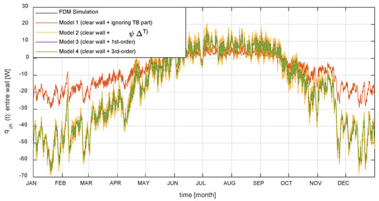
Figure 13.
Heat flow through the entire wall (one year).
For a more detailed illustration, the results for a specific period (6 days from August 15 to August 20 in summer and 6 days from January 15 to January 20 in winter) are shown in Figure 14 and Figure 15. It can be seen that the results of the third-order model are almost identical to those of the FDM model. Further, the results of the first-order model are slightly more inaccurate than those of the third-order model but are significantly more accurate than those of Model 1 and Model 2. Figure 16 shows the residual of each model error over time for one year. To quantitatively confirm the accuracy of each model result, the root means square error (RMSE) is obtained, as shown in Table 9.
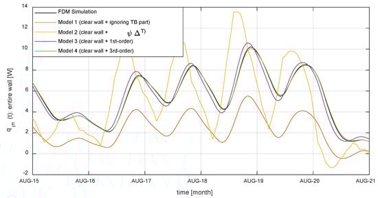
Figure 14.
Heat flow through the entire wall (Summer).
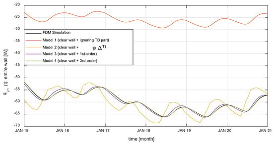
Figure 15.
Heat flow through the entire wall (Winter).
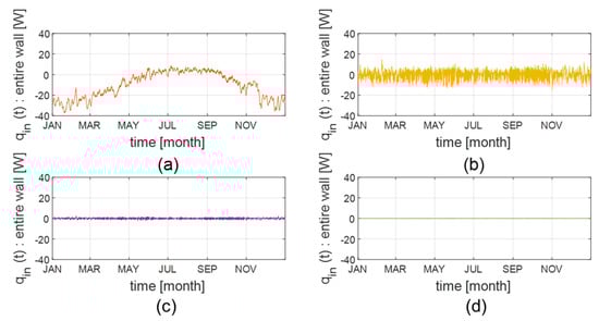
Figure 16.
Residual of annual heat flow through the entire wall: (a) Model 1; (b) Model 2; (c) Model 3; (d) Model 4.
Table 9.
The TB analysis method for the models and RMSE of each model for annual heat flow.
The proposed method is, thus, verified by various responses, proving that its accuracy is significantly improved compared to existing TB analysis methods. This means that even under dynamic conditions, the heat flow through the entire wall can be expressed as a linear combination of the heat flow through the clear wall and the heat flow through the TB parts, as in steady-state analysis. It also means that it is possible to create a dynamic model of the TB by separating only the heat flow through the TB parts. The TB part is a part described in terms of heat flow rather than a geometric part of actual TB, and heat flow through the TB part is defined as heat flow through the entire wall, excluding heat flow through the clear wall. The range of the TB part is also worth discussing. K. Martin suggested that the location of the cut-off plane for a correct dynamic thermal characterization of a TB occurs where the inner surface temperature deviates by more than 0.2 K [25]. This proposal is well suited to explain the dynamic properties of the TB itself and can be seen as a way to define the range of the TB part. Since this paper discusses how to apply the TB part to the BES, it is necessary to define the TB part by understanding how to analyze the entire wall and the clear wall in the BES. In the BES, when analyzing a wall, 1D analysis is performed by entering the area of the wall along the interior or exterior dimension system. This means that the heat flow through the part corresponding to the interior or exterior dimension is already analyzed and reflected in the BES. Indeed, the TB should be analyzed in the BES to provide an additional analysis of the entire wall minus the part that is already being analyzed. Otherwise, the range for analyzing the clear wall in the BES must also be modified, which may not be a simple method for the BES users. Therefore, to apply the TB model and analysis method to the BES, it is necessary to define the TB part in terms of heat flow according to the existing method for analyzing walls in the BES. The heat flow through the TB parts is also defined as the heat flow through the entire wall, excluding the heat flow through the 1D wall calculated by the BES program.
In this study, the TB part is assumed to be an LTI system. This is not very different from the existing equivalent wall concept, where the equivalent wall has a simple 1D multilayer structure and the same thermal properties as an actual wall [14]. As shown in the Appendix A, the system order and the differential order of the LTI system have the same meaning as the number of equivalent wall layers or equivalent heat capacities. This is also the same as changing a large number of differential equations to a low-order model under a state-space approach. These various methods have different approaches, but, consequently, they can be converted into an LTI system to analyze a thermal bridge. Some methods use a step response or sinusoidal response to verify the proposed method [24,37]. This paper’s method inversely estimates a system that fits the step response.
The TB part was estimated by performing SI with the input data (step input) and output data. As mentioned earlier, this is not very different from curve fitting. For example, if a first-order system is estimated, the solution of the first-order differential equation is , which thus involves the process of finding the and that best fit the output data graph. If a second-order system is estimated, then the solution form of the second-order differential equation is slightly more complicated but can also find the coefficients that fit the graph.
This method has a limitation in that it requires dynamic numerical analysis. Nevertheless, fewer data and time resources are needed because only the simulation period is required to perform system identification using a step-response, rather than a year-long numerical analysis of the building envelope. In addition, this process is highly useful because it can be applied to various simulations in the BES using the results obtained through a single short dynamic numerical analysis, rather than performing a dynamic numerical analysis for every case.
7. Conclusions
A thermal bridge modeling and dynamic analysis method that can be efficiently applied to a BES program have been developed. Since the BES program is a program that analyzes energy in a building, the study has been conducted with interest only in the heat flow, which is the energy entering the room through the TB. In addition, since the BES program is a 1D platform, the focus is on making a simple model that enables a 1D analysis of heat flow through a TB that requires 3D analysis.
Similar to the steady-state analysis method, a dynamic analysis method for TB has been proposed as a method of calculating the heat flow by excluding the heat flow through the clear wall from the heat flow through entire wall. Furthermore, a TB model has been proposed and validated as a transfer function (TBTF), assuming the TB part as an LTI system. The parameter of TBTF can be estimated by system identification. The procedure of the TB modeling is introduced in four steps: the disaggregation stage, the dynamic simulation stage, the model construction stage and the system identification stage.
The TB model and the dynamic analysis method have been studied in consideration of the simplicity and accuracy of the model, the simulation time (including implementation time) and the efficiency applicable to BES. In these four aspects, the proposed method can draw the following conclusions.
- The proposed TB model is simple because it can be expressed with several parameters according to the system order as a transfer function. When the TB is modeled with a third-order system, the TB model can be expressed with only four parameters (one parameter for the numerator and three parameters for the denominator).
- The accuracy of the proposed TB model depends on the system order, but the normalized root mean square error of the step response is more than 99% (99.76% for the third-order system and 99.97% for the fourth-order system). The amplitude error of the sinusoidal response is −4.78% for the third-order system and −0.52% for the fourth-order system, and the time shift error is 360 s for the third-order system and 0 s for the fourth-order system. In addition, since the RMSE is 0.1 W in the system response of annual outdoor temperature, it can be said that the proposed TB model has sufficient accuracy.
- In the method of this study, thermal fields calculation software capable of 3D dynamic analysis is needed to obtain input/output data required for the system identification process, which is a step to estimate the parameter of TBTF. In the explanatory example, since the steady state is reached in a simulation period of about 5 days, a simulation of about 10 days can sufficiently implement the proposed method. Thereafter, using the estimated TBTF, the simulation time for one year is only a few seconds. Therefore, the computer memory and time-consuming problems are alleviated rather than directly performing 3D thermal fields calculation for one year.
- The proposed method is a method that calculates only the heat flow that additionally enters through the TB, excluding the heat flow through the clear wall that can be analyzed in BES. In terms of heat flow, since the heat flow through the entire wall is separated into heat flow through the clear wall and heat flow through the TB part and linearly combined, the heat flow through the entire wall can be calculated separately and simply added. Therefore, BES program code can be used as it is to calculate the heat flow through the clear wall, and dynamic analysis of TB is possible by adding additional program code for calculating TBTF to BES program. There is an efficiency applicable to BES in that it simply adds a program code that calculates TBTF while continuing to use the existing code of the BES program that analyzes the clear wall.
We also compared the simulation results of the heat flow through the entire wall for one year using the models proposed in this study (the first-order system and the third-order system for the TB part) and the currently used dynamic analysis model for TB (the model that ignored the TB and the model that analyzes the TB in steady-state). The annual simulation results conclude that:
- The accuracy of the proposed models is significantly higher than that of other models. The RMSE of the model that ignored the TB is 16 W, and the RMSE of the model that analyzes the TB in steady-state is 4.3 W, whereas the RMSE of the proposed model is 0.69 W for the first-order system model and 0.1 W for the third-order system model.
- Among the proposed models, the first-order system model is more inaccurate than the third-order system model, but it is clearly more accurate than other models.
- The accuracy of the dynamic analysis of TB is lower in winter than in summer. The temperature difference between indoor and outdoor is larger in winter than in summer, so the amount of heat flow through the TB is increased, which reduces the accuracy of the models.
Further studies should investigate how the proposed method is implemented in BES and its application to TBs of various geometric shapes and materials. As suggested by the linear thermal transmittance in the steady state analysis of a TB [10,33], a study to find the TBTF corresponding to each type by sorting the various types of TBs into several types seems to be necessary. Additional research is needed for the TB model when the indoor temperature is a time-varying variable.
Author Contributions
Conceptualization, methodology, software and writing—original draft preparation, H.K.; conceptualization, writing—review and editing, supervision, M.Y. All authors have read and agreed to the published version of the manuscript.
Funding
This research was supported by Basic Science Research Program through the National Research Foundation of Korea (NRF) funded by the Ministry of Education (NRF-2018R1D1A1A09083184).
Conflicts of Interest
The authors declare no conflict of interest.
Appendix A. Thermal Network Model and the LTI System
The thermal network model is a traditional model that uses virtual heat resistance (R) and heat capacity (C) to analyze the heat transfer phenomenon through an electrical analogue. This model has been applied to model the walls of buildings, whole buildings and various components in the BES. The thermal network model can also be converted to an LTI system (via the LTI differential equation). Here, the process for converting the 2R1C model (model consisting of 2 heat resistance and 1 heat capacity) and the 3R2C model (model consisting of 3 heat resistance and 2 heat capacity) to an LTI system is briefly described.

Figure A1.
The 2R1C model.
Figure A1.
The 2R1C model.

- 2R1C model
Equation (A1) describes the state of the model, and Equation (A2) describes the output of the model. Assuming that the indoor temperature () is a constant, introducing the temperature difference
and recognizing that , it follows that
Equations (A4) and (A5) are the governing equations for temperature difference. Given , eliminate by substituting Equation (A5) into Equation (A4):
Then, the LTI system for the 2R1C model can be provided as Equation (A6).

Figure A2.
The 3R2C model.
Figure A2.
The 3R2C model.

- 3R2C model
Equations (A7) and (A8) describe the state of the model, and Equation (A9) describes the output of the model. Assuming that the indoor temperature () is a constant, introducing the temperature difference
and recognizing that and , it follows that
Equations (A11)–(A13) are the governing equations for temperature difference. When , eliminate by substituting Equation (A13) into Equation (A12); then, Equation (A12) becomes
When Equation (A14) is expressed in terms of , the following equation can be obtained:
Again, eliminate and by substituting Equations (A13) and (A15) into Equation (A11)
Finally, the LTI system for the 3R2C model can be given as Equation (A16).
References
- Crawley, D.B.; Hand, J.W.; Kummert, M.; Griffith, B.T. Contrasting the capabilities of building energy performance simulation programs. Build. Environ. 2008, 43, 661–673. [Google Scholar] [CrossRef]
- Harish, V.; Kumar, A. A review on modeling and simulation of building energy systems. Renew. Sustain. Energy Rev. 2016, 56, 1272–1292. [Google Scholar] [CrossRef]
- Foucquier, A.; Robert, S.; Suard, F.; Stéphan, L.; Jay, A. State of the art in building modelling and energy performances prediction: A review. Renew. Sustain. Energy Rev. 2013, 23, 272–288. [Google Scholar] [CrossRef]
- Balaji, N.; Mani, M.; Reddy, B.V. Dynamic thermal performance of conventional and alternative building wall envelopes. J. Build. Eng. 2019, 21, 373–395. [Google Scholar] [CrossRef]
- Al-Saadi, S.N.; Zhai, Z.J. Modeling phase change materials embedded in building enclosure: A review. Renew. Sustain. Energy Rev. 2013, 21, 659–673. [Google Scholar] [CrossRef]
- Li, Q.; Rao, J.; Fazio, P. Development of HAM tool for building envelope analysis. Build. Environ. 2009, 44, 1065–1073. [Google Scholar] [CrossRef]
- Wang, H.; Zhai, Z.J. Advances in building simulation and computational techniques: A review between 1987 and 2014. Energy Build. 2016, 128, 319–335. [Google Scholar] [CrossRef]
- Bergman, T.L.; Incropera, F.P.; DeWitt, D.P.; Lavine, A.S. Fundamentals of Heat and Mass Transfer; John Wiley & Sons: Hobokene, NJ, USA, 2011. [Google Scholar]
- Quinten, J.; Feldheim, V. Dynamic modelling of multidimensional thermal bridges in building envelopes: Review of existing methods, application and new mixed method. Energy Build. 2016, 110, 284–293. [Google Scholar] [CrossRef]
- ISO. 10211: 2017 Thermal Bridges in Building Construction–Heat Flows and Surface Temperatures–Detailed Calculations; ISO: Geneva, Switzerland, 2017. [Google Scholar]
- Kosny, J.; Desjarlais, A. Influence of architectural details on the overall thermal performance of residential wall systems. J. Therm. Insul. Build. Envel. 1994, 18, 53–69. [Google Scholar] [CrossRef]
- Ge, H.; Baba, F. Effect of dynamic modeling of thermal bridges on the energy performance of residential buildings with high thermal mass for cold climates. Sustain. Cities Soc. 2017, 34, 250–263. [Google Scholar] [CrossRef]
- Martin, K.; Erkoreka, A.; Flores, I.; Odriozola, M.; Sala, J. Problems in the calculation of thermal bridges in dynamic conditions. Energy Build. 2011, 43, 529–535. [Google Scholar] [CrossRef]
- Kośny, J.; Kossecka, E. Multi-dimensional heat transfer through complex building envelope assemblies in hourly energy simulation programs. Energy Build. 2002, 34, 445–454. [Google Scholar] [CrossRef]
- Crawley, D.B.; Lawrie, L.K.; Pedersen, C.O.; Winkelmann, F.C. Energy plus: Energy simulation program. Ashrae J. 2000, 42, 49–56. [Google Scholar]
- Fiksel, A.; Thornton, J.; Klein, S.; Beckman, W. Developments to the TRNSYS simulation program. J. Sol. Energy Eng. 1995, 117, 2. [Google Scholar] [CrossRef]
- Mitchell, R.; Kohler, C.; Curcija, D.; Zhu, L.; Vidanovic, S.; Czarnecki, S.; Arasteh, D.; Carmody, J.; Huizenga, C. THERM 7/WINDOW 7 NFRC Simulation Manual; Lawrence Berkeley National Lab.(LBNL): Berkeley, CA, USA, 2017. [Google Scholar]
- Standaert, P. PHYSIBEL Software Pilot Book; PHYSIBEL: Gent, Belgium, 2010. [Google Scholar]
- Zirkelbach, D.; Schmidt, T.; Kehrer, M.; Künzel, H. Wufi® Plus–Manual; Fraunhofer-Gesellschaft: Munchen, Germany, 2007. [Google Scholar]
- TRISCO v11.0w Manual; PHYSIBEL: Gent, Belgium, 2005.
- VOLTRA v6.0w Manual; PHYSIBEL: Gent, Belgium, 2006.
- Kossecka, E.; Kosny, J. Equivalent wall as a dynamic model of a complex thermal structure. J. Therm. Insul. Build. Envel. 1997, 20, 249–268. [Google Scholar] [CrossRef]
- Nagata, A. A simple method to incorporate thermal bridge effects into dynamic heat load calculation programs. In Proceedings of the International IBPSA Conference, Montreal, QC, Canada, 15–18 August 2005; pp. 817–822. [Google Scholar]
- Xiaona, X.; Yi, J. Equivalent slabs approach to simulate the thermal performance of thermal bridges in building constructions. IbpsaProc. Build. Simul. 2007, 10, 287–293. [Google Scholar]
- Martin, K.; Escudero, C.; Erkoreka, A.; Flores, I.; Sala, J. Equivalent wall method for dynamic characterisation of thermal bridges. Energy Build. 2012, 55, 704–714. [Google Scholar] [CrossRef]
- Alhawari, A.; Mukhopadhyaya, P. Thermal bridges in building envelopes–An overview of impacts and solutions. Int. Rev. Appl. Sci. Eng. 2018, 9, 31–40. [Google Scholar] [CrossRef]
- Simões, N.; Prata, J.; Tadeu, A. 3D Dynamic Simulation of Heat Conduction through a Building Corner Using a BEM Model in the Frequency Domain. Energies 2019, 12, 4595. [Google Scholar] [CrossRef]
- Baba, F. Dynamic Effect of Thermal Bridges on the Energy Performance of Residential Buildings. Master Thesis, Concordia University, Montreal, QC, Canada, 2015. [Google Scholar]
- Iodice, P.; Massarotti, N.; Mauro, A. Effects of inhomogeneities on heat and mass transport phenomena in thermal bridges. Energies 2016, 9, 126. [Google Scholar] [CrossRef]
- Bienvenido-Huertas, D.; Quiñones, J.A.F.; Moyano, J.; Rodríguez-Jiménez, C.E. Patents analysis of thermal bridges in slab fronts and their effect on energy demand. Energies 2018, 11, 2222. [Google Scholar] [CrossRef]
- Gao, Y.; Roux, J.; Zhao, L.; Jiang, Y. Dynamical building simulation: A low order model for thermal bridges losses. Energy Build. 2008, 40, 2236–2243. [Google Scholar] [CrossRef]
- DOE. EnergyPlus Version 9.0.1 Documentation: EnergyPlus Engineering Reference; US Department of Energy: Washington, DC, USA, 2016.
- ISO. 14683: 2017 Thermal Bridges in Building Construction-Linear Thermal Tansmittance-Simplified Methods and Default Values; ISO: Geneva, Switzerland, 2017. [Google Scholar]
- Ogata, K. System Dynamics; Pearson/Prentice Hall Englewood Cliffs: Upper Saddle River, NJ, USA, 2004; Volume 13. [Google Scholar]
- Li, X.Q.; Chen, Y.; Spitler, J.; Fisher, D. Applicability of calculation methods for conduction transfer function of building constructions. Int. J. Therm. Sci. 2009, 48, 1441–1451. [Google Scholar] [CrossRef]
- Tangirala, A.K. Principles of System Identification: Theory and Practice; CRC Press: Boca Raton, FL, USA, 2018. [Google Scholar]
- Martinez, R.G.; Riverola, A.; Chemisana, D. Disaggregation process for dynamic multidimensional heat flux in building simulation. Energy Build. 2017, 148, 298–310. [Google Scholar] [CrossRef]
- Matlab, M. MATLAB R2018b; Mathworks: Natick, MA, USA, 2018. [Google Scholar]


© 2020 by the authors. Licensee MDPI, Basel, Switzerland. This article is an open access article distributed under the terms and conditions of the Creative Commons Attribution (CC BY) license (http://creativecommons.org/licenses/by/4.0/).