Simulation of the GOx/GCH4 Multi-Element Combustor Including the Effects of Radiation and Algebraic Variable Turbulent Prandtl Approaches

Abstract

Multi-element thrusters operating with gaseous oxygen (GOX) and methane (GCH4) have been numerically studied and the results were compared to test data from the Technical University of Munich (TUM). A 3D Reynolds Averaged Navier–Stokes Equations (RANS) approach using a 60° sector as a simulation domain was used for the studies. The primary goals were to examine the effect of the turbulent Prandtl number approximations including local algebraic approaches and to study the influence of radiative heat transfer (RHT). Additionally, the dependence of the results on turbulence modeling was studied. Finally, an adiabatic flamelet approach was compared to an Eddy-Dissipation approach by applying an enhanced global reaction scheme. The normalized and absolute pressures, the integral and segment averaged heat flux were taken as an experimental reference. The results of the different modeling approaches were discussed, and the best performing models were chosen. It was found that compared to other discussed approaches, the BaseLine Explicit Algebraic Reynolds Stress Model (BSL EARSM) provided more physical behavior in terms of mixing, and the adiabatic flamelet was more relevant for combustion. The effect of thermal radiation on the wall heat flux (WHF) was high and was strongly affected by spectral models and wall thermal emissivity. The obtained results showed good agreement with the experimental data, having a small underestimation for pressures of around 2.9% and a good representation of the integral wall heat flux.

1. Introduction

The design and optimization of rocket propulsion devices is a complex procedure that nowadays also includes the numerical simulation of flow and tough physical phenomena as a very important part of the process. This is mainly due to the significant reduction of the cost and time needed for overall testing, production, and development cycle. The main criteria that show if the code can be applied for rocket thrusters are wall heat transfer, combustion efficiency, specific impulse, and pressure representation. The tool should both accurately predict the parameter distribution inside the combustor and satisfy typical needs of design engineers such as robust and stable operation and as small as possible calculation times. Numerical codes, therefore, should be validated for the criteria above-mentioned and the most suitable models of physical phenomena should be chosen.

Conversely, the methane–oxygen fuel pair is now considered as prospective for rocket propulsion. In recent years, the Space Propulsion Division of TUM has been working experimentally and numerically on various aspects of methane/oxygen combustion. Among these, a GCH4/GOx multi-element injector test case was chosen for the RANS-based numerical assessment in our study. The reason to choose this experiment was not only the well-described setting that is well suited for numerical verification, but also the fact that numerous research groups have also used this data, which is extremely useful to efficiently compare the different methodologies and their results, and finally choose appropriate approaches for our problems. A paper by Silvestri et al. [1,2] gives detailed data concerning the test bench and experimental setting and therefore only a short description is given here in the “test case” section.

Recently, some numerical studies have already been made to examine the effect of modeling approaches using both a single-injector test case [3,4,5] and a multi-element setting [6,7,8,9]. Furthermore, some extensive analyses have been performed concerning the PennState and Mascotte test cases [10,11,12]. All authors have given great attention to the turbulence modeling and state its high influence on the mixing intensity and therefore on the predicted heat fluxes and pressures. Another obvious and important statement is the high impact of the approach to model the interaction of turbulence and chemistry and of the chemical kinetic scheme itself.

Additionally, some research has been made aiming at the influence of the coefficients that account for turbulent diffusion such as turbulent Schmidt and Prandtl numbers [13,14,15,16,17,18,19]. An essential impact of these parameters was observed on the wall heat fluxes and pressures, coupled with the variation of the thermodynamic and reactive parameters inside the combustor. The papers either provide a sensitivity study to choose the correct values or propose methods for their local variation.

Additionally, computational fluid dynamics (CFD) is now extremely widespread in all fluid dynamics applications, especially in industrial purposes of rocket combustion modeling. The industry requires such predictions to be fast, but still sufficiently precise to allow their implementation into a routine design optimization process. Such approaches are needed during the early phases of the design process. Therefore, in our paper, the cheapest and most robust techniques were tested to establish a modeling methodology of such complex phenomena applicable for industrial applications and purposes. Such industry demands also drive the usage of most universal approaches for any processes described by the computational model, as changes in the geometry and mass flows during the optimization might change the parameter field significantly. This makes the application of the approaches for locally variable diffusion coefficients even more urgent.

The number of papers accounting for radiative heat transfer in such studies is limited. Zhukov [10] used a P1 Gray radiation heat transfer (RHF) model and noted some effect on the heat flux, whereas due to some uncertainty in the existing wall roughness, no reliable conclusions could be drawn. Thellmann [20] studied the hydrogen–oxygen and methane–oxygen combustion at high pressures, which resulted in radiative to total heat flux ratios up to 9%. Leccesse et al. [21] also studied these fuel pairs and found that the contribution of the RHF was up to 15% for the described cases. Some other studies have referred to general RHF evaluation in turbulent combustion tests [22,23,24,25] and showed significant influences that should be accounted for.

Most of the research activities that focused on single and multi-injector test cases had a grid resolution near the wall, which met the $y^{+}\approx 1$ condition [3,4,6,7,8,25]. Some groups have focused on the development of special wall-functions that they implemented in their large Eddy simulations (LES) [26,27,28,29,30,31,32]. However, the usage of wall functions for RANS simulations can both accelerate and stabilize the optimization workflow. As wall function-based simulations combined with a wide variety of modeling approaches have not yet been performed on these cases, it was considered as important in this study.

Nearly all described studies used two-equation linear turbulence models to account for the turbulence phenomena. The significant influence of turbulence modeling on the mean pressure was noticed, which was due to improved or worsened mixing efficiency. Generally, a $k-\epsilon$ model is considered to be giving more physical values of turbulence viscosity, and therefore, the mixing intensity. In this paper, the turbulence field was estimated by three models—the popular Menter’s $k-\omega$ Shear stress transport (SST), the $k-\epsilon$, and the BSL EARSM [33]—to include the anisotropy effects. The use of the BSL EARSM approach is driven by its satisfactory convergence behavior and reduced CPU demands compared to straight Reynolds stress models.

Therefore, the motivation and goals of this study follow the industrial simulation requirements for robustness, low calculation time, and sufficiently reliable simulation results, especially in terms of pressure and wall heat flux inside the combustor, and can be summarized as follows: (1) implementation of locally variable turbulent Prandtl approaches and comparison with its constant values; (2) further estimation of turbulence modeling methods based on the comparison of commonly used two-equation models and a BSL EARSM method; (3) estimation of the radiative heat transfer impact on the wall heat flux; and (4) all these being coupled with a wall-function based near-wall modeling approach for both the velocity and thermal boundary layer to test the capability of such methods in the high pressure and high thermal gradient environment.

2. The Test Case

The chosen test case was developed as a part of the Sonderforschungsbereich Transregio 40 (SFB-TRR 40) program. It includes seven coaxial gaseous methane and gaseous oxygen injectors, which allowed us to study effects such as the injector–injector and injector–wall interaction, which is highly important for turbulence–chemistry interaction and the wall heat transfer. The chamber diameter is 30 mm, whereas each injector consists of a central oxygen injector, a post wall, and a concentric methane injector. The oxygen injector has a diameter of 4 mm while the methane injector has a 5 mm inner and 6 mm outer diameter, respectively. The peripheral injectors had their axis 9 mm off the main axis. The throat diameter was equal to 19 mm, determining the chosen contraction ratio of 2.5. The view of the combustor is shown in Figure 1. One of the main features of the design is that it contains four cylindrical water-cooled segments and a nozzle segment, allowing the determination of the integral wall heat flux. The total length of 381 mm makes it possible for the coaxially injected jets to mix properly and react.

For the present study, a load point corresponding to the mixture ratio of 2.65 and the mean pressure of 18.3 bar was chosen. Therefore, the total mass flows were 0.211 kg/s and 0.08 kg/s for oxygen and methane, respectively, while the injection temperatures were 259.4 K for oxygen and 237.6 K for methane. The experimentally determined data included heat flux for each segment, mean pressure, wall pressure distribution, wall temperatures, and methane/oxygen flow rates. References [1,2,6,7,8] give the full information about the experimental data available.

3. Numerical Setup

The numerical simulations were carried out via the Ansys CFX [33] three-dimensional coupled algebraic multigrid solver. The Favre-averaged equations were solved in a steady-state setting.

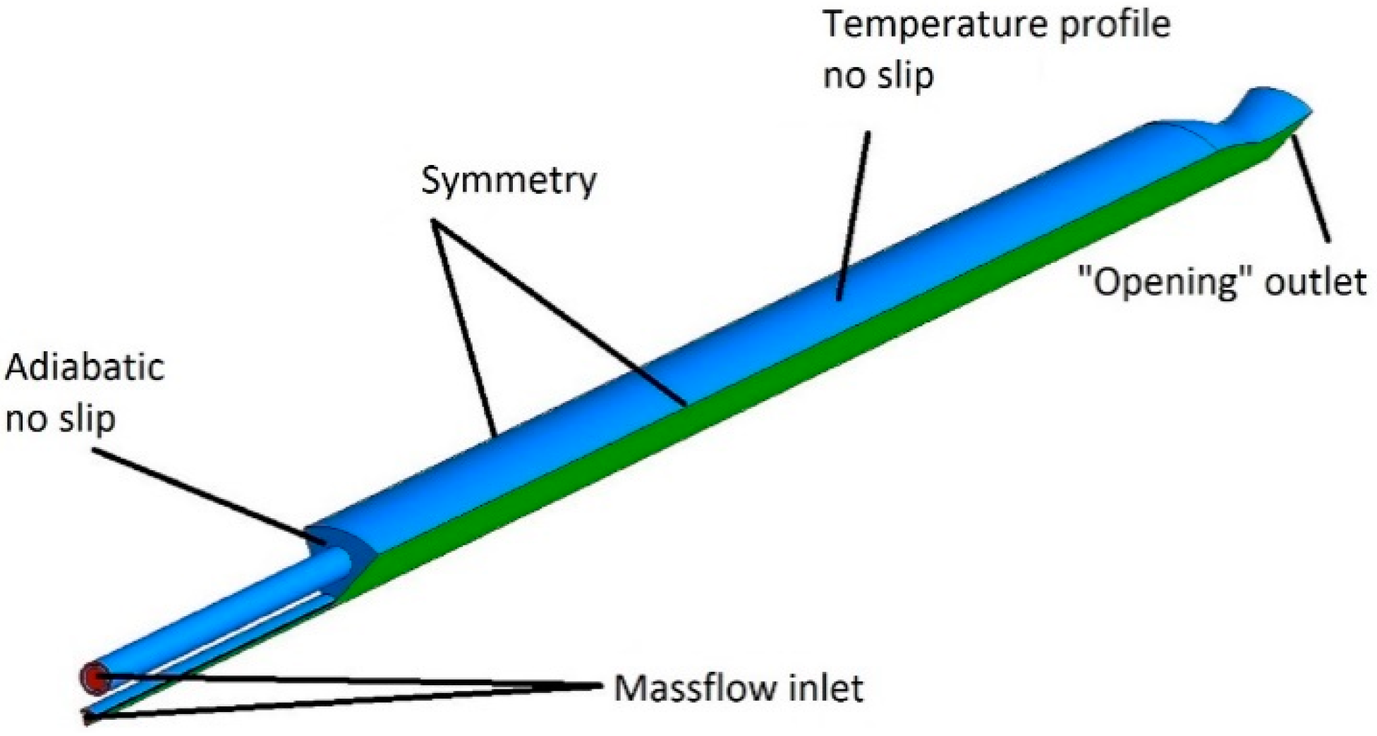
3.1. Simulation Domain

The domain chosen for the computations resolved a 60° sector of the combustor, which included one peripheral injector and 1/6 of the central injector. To account for the velocity profile at the injection point, the injector grid domains were also included. As described in Figure 2, the symmetry boundaries were applied to the planes corresponding to ±30° from the injector’s radial position. This symmetrical approach has already been widely used to study rocket combustors numerically, both in this particular case and in others [3,4,5,6,7,8]. The experimental mass flows and temperatures were set for the propellant inlets and an “opening” type for the nozzle orifice boundary condition was set. At the thruster wall, the non-slip condition with the experimental temperature profile shown in Figure 3 was reproduced. A no-slip adiabatic approach was applied to other walls. Due to the previously detected ambiguities in the nozzle heat flux estimations and the need to account for the conjugate heat transfer [6,7,8], no comparison between the experimental and CFD data was applied. The nozzle temperature was set equal to the last value of the temperature profile in the cylindrical part. The fuel and products were assumed as ideal gases, whereas the kinetic theory based transport properties were used for ${\mathrm{O}}_2$ and ${\mathrm{CH}}_4$.

The approximate grid size of 3.3 mio. (4th mesh) excluding injectors, corresponding to a hexahedral mesh, was chosen after a convergence study outlined in

Table 1. Mesh independence study data.

Criterion	Coarse (1st)	2nd	3rd	4th	Fine (5th)
Num. of cells, mio.	0.8017	1.708	2.503	3.2803	6.92
Max. pressure, bar	16.38	17.32	17.59	17.65	17.72
Integral WHF, MW	0.151	0.157	0.1612	0.1621	0.1625
Relative error, max pressure %	---/---	5.43	1.53	0.34	0.40
Relative error, integral WHF %	---/---	3.82	2.61	0.56	0.25

, based on the maximal pressure and integral wall heat flux criteria. The relative error was calculated as in Equation (1).

$$\epsilon =\frac{{\phi }_i-{\phi }_{i-1}}{{\phi }_i}*100\%$$

(1)

where $i$ is the number of the grid studied and $\phi$ is the studied parameter. The adiabatic flamelet approach for combustion, shear-stress transport for turbulence, and default turbulent Prandtl combined with a P1 Weighted-Sum-of-Gray-Gases (WSGG) radiation approach were used for grid study calculations.

One of the main issues of the current study was to check if the general wall function approach can be coupled with RANS for the wall heat flux estimation, which would make the optimization routine computations in the industry faster and easier. Thus, a mesh corresponding to the non-dimensional wall distance values of $y^{+}\approx 45\dots 410$ was applied, making use of the default wall-function based near-wall treatment of the numerical models. In Figure 4, a front view of the mesh is shown.

3.2. Numerical Models

As for the turbulent Prandtl number, mostly variations of the constant values or use of the differential models are present in the combustion-related studies [13,14,15,16,17,18,19] among the observed papers. The second type of approach can be numerically expensive in some cases, and so this was not included in our study. The first, in contrast, does not account for turbulent diffusion effects variation along with the computational domain, which can be crucial for the variations of the geometry and operational point during optimization and for the development of a relatively universal approach for turbulent diffusion coefficients. Thus, two algebraic models were implemented and compared to three constant values of turbulent Prandtl: 0.3, 0.6, and 0.9. These two models, namely the Wassel–Catton (WC) (2) and the Kays–Crawford (KC) (3), had been previously studied by D. Yoder [34,35,36] and showed satisfactory performance (compared to the differential models studied) for near-wall, jet, and pipe flows. Additionally, both models can be considered as promising, as they are faster and more robust than the differential ones, while still accounting for the locally variable turbulent Prandtl.

$$P{r}_t=\frac{C_3}{C_{1}Pr}[1-\exp (\frac{-C_4}{{\mu }_t/{\mu }_l})]{[ 1-\exp (\frac{-C_2}{\left(\frac{{\mu }_t}{{\mu }_l}\right)Pr})]}^{-1}$$

(2)

$$P{r}_t={\{\frac{1}{2P{r}_{T\infty }}+\frac{CP{e}_t}{\sqrt{P{r}_{T\infty }}}-{\left(CP{e}_t\right)}^2\left[1-\exp \left(\frac{-1}{CP{e}_t\sqrt{P{r}_{T\infty }}}\right)\right]\}}^{-1}$$

(3)

where $C_1$ = 0.21; $C_2$= 5.25; $C_3$ = 0.2; $C_4$ = 5; $Pr$ is the molecular Prandtl number; ${\mu }_t$ is the eddy viscosity; ${\mu }_l$ is the dynamic viscosity; C = 0.3; $P{r}_{T\infty }$ = 0.85; and $P{e}_t=\frac{{\mu }_t}{{\mu }_l}Pr$ is the turbulent Peclet number.

The high and non-homogenous temperature values inside the rocket combustors compel researchers to account for radiative heat transfer. Here, to study its influence and the impact of a spectral modeling approach, several cases were numerically compared: the non-radiative and two radiative ones. The radiative simulations were done with the Gray spectral model and the WSGG method. The P1 differential model was used due to its applicability to a wide range of optical thicknesses and its robust behavior during simulations. No scattering was considered in this study as no particles were introduced; studies of radiation heat transfer without scattering have previously been done for gaseous fuels and have given relevant results [20]. The default Gray spectral model was used, whereas the implemented WSGG refers to the paper by Centeno et al. [37]. In this paper, the authors introduced a four-gray-gases WSGG model with weighting factors for each gray gas derived as a polynomial function of temperature. The absorption coefficients depend upon the partial pressures of most radiating species, ${\mathrm{H}}_2\mathrm{O}$ and ${\mathrm{CO}}_2$. For the absorbing and emitting, non-scattering case, the radiation transfer equation would have the form [33]:

$$\frac{d{I}_{\upsilon }\left(\mathit{r},\mathit{s}\right)}{ds}=-K_a*I_{\upsilon }\left(\mathit{r},\mathit{s}\right)+K_{a\upsilon }*I_b\left(\upsilon ,T\right)$$

(4)

where υ is the frequency; r is the position vector; s is the direction vector; s is the path length; $K_a$ is the absorption coefficient; $K_{a\upsilon } \mathrm{is}$ the blackbody absorption coefficient; $I_{\upsilon }$ is the spectral radiation intensity; and $I_b$ is the blackbody emission intensity. The weighting factors were determined by the relation below:

$$a_j\left(T\right)={\displaystyle \sum }_{i=1}^5{b}_{j,i}{T}^{i-1}$$

(5)

where $b_{j,i}$ are the polynomial coefficients taken from reference [37]. The absorption coefficients were introduced by the equation:

$$k_j=\left(p_{H_{2}O}+p_{C{O}_2}\right)\ast k_{p,j},$$

(6)

where $p_{C{O}_2}$ and $p_{H_{2}O}$ were ${\mathrm{CO}}_2$ and ${\mathrm{H}}_2\mathrm{O}$ partial pressures, respectively, and $k_{p,j}$ was taken from [37].

It is important to note that nevertheless, the WSGG coefficients were obtained for constant $p_{H_{2}O}$ to $p_{C{O}_2}$ ratio ($\frac{p_{H_{2}O}}{p_{C{O}_2}}=2$) and the dependence of the absorption coefficient upon the partial pressures of species where the concentrations are derived locally, make this approach applicable for non-homogenous combustion studies. The comparison of results with the non-homogenous ratio based constants simulation gave good agreement and the constant ratio approach was recommended by the developers to save computational resources. In general, this model can be enhanced or revised to accomplish best fit to the test measurements. The Gray spectral model instead assumes that the radiative properties are equal for each gas. Another important point is the setting of the wall emissivity, as this value identifies the amount of radiative heat absorbed and reflected by the wall. Though it is known that the inner part of the chamber consisted of a CuCrZr alloy [7], the exact absorbing-emitting properties could not be obtained in the experiments. Furthermore, the absorbing-emitting properties can vary along the thruster during testing because of the temperature differences and the formation of oxides on the surface. Therefore, three values of wall emissivity were implied to get a sensitivity picture for the final estimation of radiative heat flux impact. Additionally, in some simulations, a unity emissivity value was set for both spectral models to get a higher limit of radiative wall heat flux. During all studies, a unity wall radiation diffuse fraction was set, which means that the reflected energy is spread diffusely.

In this paper, two general approaches were used to model chemical reactions. One is the adiabatic flamelet approach, whose underlying theory follows the diffusion laminar flame basis coupled with the turbulent field by a presumed probability density function and is now a widely applied method for combustion simulation [33,38,39]. Its main advantage is high computational performance while still considering full kinetics due to only two scalars to transport: the mixture fraction and mixture fraction variance. The turbulence–chemistry non-equilibrium interaction was accounted for by the scalar dissipation rate. The C1 CH₄/O₂ kinetics was used to create a flamelet database in CFX-RIF software.

Another combustion model used was an enhanced eddy-dissipation based approach [33,40]. The global reaction includes several species—OH, CO, H, ${\mathrm{H}}_2$, O, ${\mathrm{O}}_2$,${ \mathrm{CO}}_2,{ \mathrm{CH}}_4,{ \mathrm{H}}_2\mathrm{O}$. The procedure to derive the global reaction equation is as follows: (a) a thermodynamic 1-dimensional calculation is done in a gas-thermodynamic code (here a rocket propulsion analysis software [41]); (b) the species with the largest molar fractions are taken and molar fractions are used as the initial stoichiometric coefficients for the global reaction, (c) the left-side ($C{H}_4$ and $O_2$) and the right-side coefficients (for H or others) are changed to satisfy the molar balance. Due to only one global reaction, it remains fast and relatively robust while still accounting for high-temperature dissociation and the production of most participating species. The final global reaction is presented below (Equation (7)).

$$\begin{array}{c}0.2789274 \left[C{H}_4\right]+0.5576753 [O_2] =0.147891 \left[CO\right]+0.131036 \left[C{O}_2\right]+0.028828 \left[H\right]+\\ 0.0597107 \left[H_2\right]+0.433845 [H_{2}O\left]+0.0260146 \left[O\right]+ 0.072879 \right[O_2]\\ +0.0997694 \left[OH\right]\end{array}$$

(7)

4. Results and Discussion

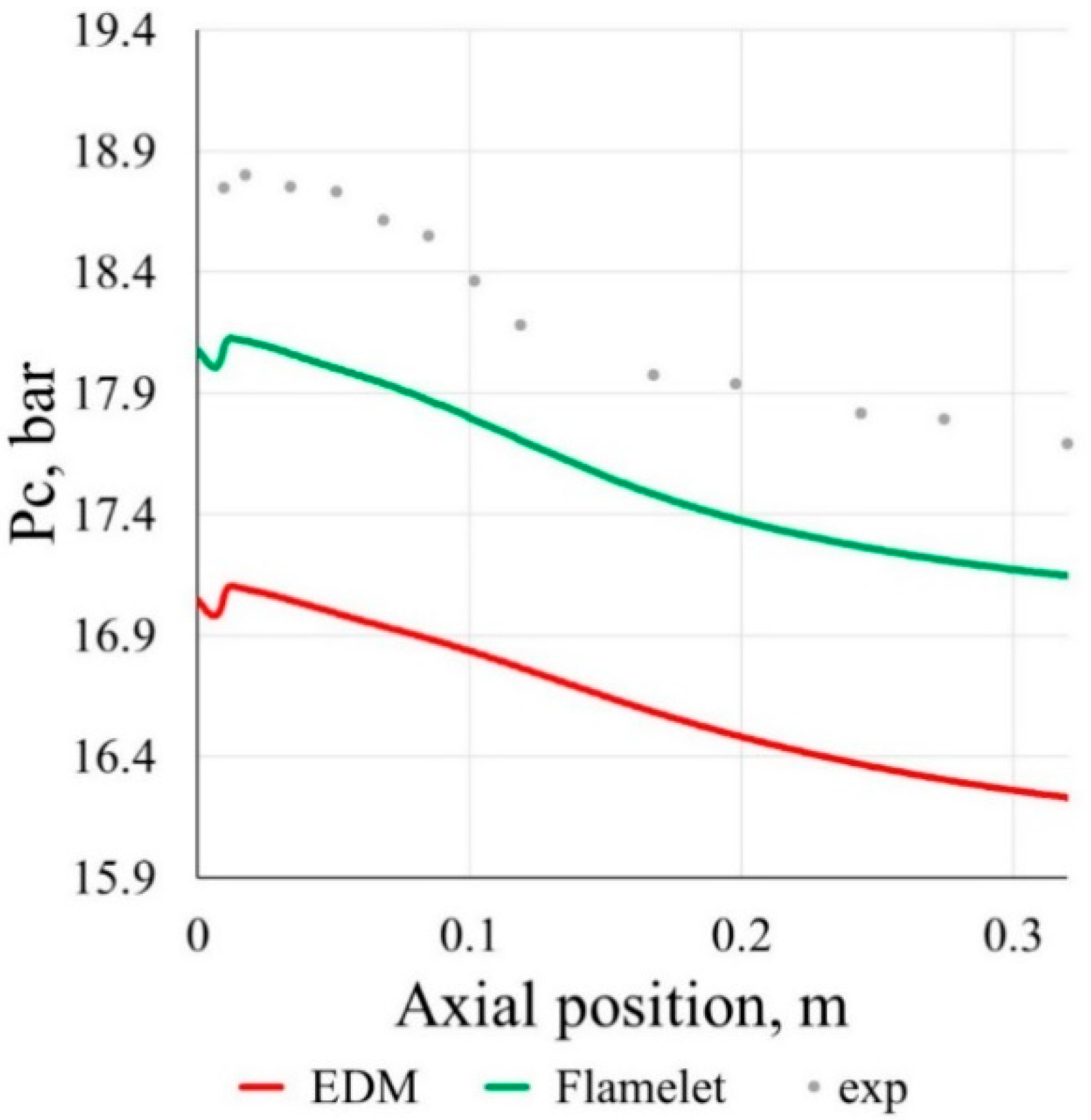
4.1. Combustion Model Effect

The impact of two combustion models was studied using the SST turbulence approach, default turbulent $P{r}_t$ 0.9 while no radiation was accounted for. Change of the approach between the adiabatic flamelet and the enhanced eddy-dissipation did not have a high influence on the normalized pressure distribution, while it significantly impacted the absolute values (Figure 5 and Figure 6). The flamelet approach gave the highest absolute pressures, which were around 0.7 bar (or <3.5%) lower than the experimental ones. The enhanced eddy dissipation model (EDM) approach with the global kinetics gave 1.5 bar (or 7.9%) less than the experimental pressures on average. Such low pressure cannot be addressed to wall heat loss: the EDM approach provides only slightly higher integral heat flux than flamelet, and the overall inconsistency between flamelet and EDM is more quantitative than qualitative (Figure 7). It is likely that the underestimation of heat flux (HF) is either due to unconsidered radiative heat transfer in this section, which would contribute into the total amount of heat flux, or poor performance of the turbulence model, which is discussed later. Another reason for wall heat flux inaccuracy might be the mechanism used for flamelet library formation, which was, however, not the focus of the study in the present paper. Additionally, the poor performance of the EDM is supposed to be due to the simplicity of the model formulation. One alternative for better accuracy could be the eddy-dissipation concept approach, which is now used for more and more reactive flow modeling studies. However, it is still not always as fast and robust as the mixture fraction type of models, which means that it can be hard to apply in some routine engineering simulations and therefore was not observed in the paper. As the library used in the flamelet approach accounts for many reactions compared to the EDM approach and is also more robust and showed better results for absolute pressures in this case, it was proposed for further use among these two. However, the applied eddy-dissipation methodology can still be utilized for the early stages of the design process.

4.2. Radiative Heat Transfer Modeling

As already mentioned, the Gray and the WSGG spectral models were used to account for radiative heat flux (RHF). A flamelet combustion model, default turbulent Prandtl number (0.9), and the SST model were used in this study. The wall emissivity for the first estimations was set to 1, which means that the full amount of RHF emitted in the flow was absorbed by the wall. The normalized pressure plot showed no effect of RHF, nor with the Gray or WSGG approach, on the axial distributions. In contrast, inclusion of RHF changed the absolute pressure values by 0.25 bar and by 0.5 bar for the WSGG and the Gray spectral models, respectively. This was due to the shift of heat loss from the flame front and transport to the wall, which is shown on the heat flux plot (Figure 8, Figure 9 and Figure 10). A notable thing is that the Gray model gave integral heat fluxes overestimated by 12.5%, whereas a no-radiation case led to underestimating it up to 15%. Some kind of compromise is found by the WSGG approach, which gives an integral HF value that is very close to the experimental, though the profile has some discrepancies in the first and last segments (

Table 2. Influence of the radiative heat transfer spectral approach.

	Radiation Model
	No Rad	Gray	WSGG 4 Gases	Exp
Integral, MW	0.1293	0.193	0.16542	0.16
Radiative/Total	---	0.3221	0.208	---

). The overestimation of the heat flux by the Gray approach can also be seen from the radiative/total heat flux ratio. This value reached 32% for the Gray model, while only 20% was given by the WSGG. This value also corresponds to the amount of RHF that the authors [37] used in their verification study. Thellmann in his thesis [20] pointed out that the radiative amount of heat flux calculated with the WSGG type of models would be around 9–10% when estimating it for the space shuttle main engine (SSME) nozzle.

On the other hand, following the considerations presented in the paper by Leccese et al. [21], the radiative/total wall heat flux approximate ratio for such pressures and chamber diameter should fall in the range between 10 and 20%. It is also important to mention that the wall emissivity might be significant in determining the heat absorbed by the wall. In this sense, as no specific value of emissivity is known, it is worth providing a sensitivity study for the emissivity. Such study for three values of wall emissivity is discussed further in Section 4.5.

Despite the fact that the relative amount of RHF is still questionable, the WSGG model gives a better fit than the unphysical Gray spectral model and should be used for further simulations. It is necessary to note that future studies should be focused on the comparison of present results with: (a) usage of the same modeling approaches implying low-Reynolds grid wall resolution; and (b) computations using higher-fidelity combustion and turbulence-chemistry interaction models. Both would lead to better estimation of the low-temperature and near-wall effects, which may contribute to the combustion efficiency and thermal emission. These could give valuable information on the behavior and the modeling limits of the “engineering-oriented” methods, which are considered in the present paper.

The inclusion of the RHF decreases the flame temperature, regardless of the spectral model used and does not affect the flame shape. The WSGG model not only predicts much lower heat flux values, but also the most emitting area is sufficiently smaller. The radiation intensity fields also show that the radiative emission is highest in the second half of the cylindrical part for both Gray and WSGG cases while the WSGG showed some variation in the radial direction starting at the half-radius. This indicates that the radiation intensity is mainly dependent on the axial coordinate, is most intensive in the core, and is not that sensitive to the near-wall concentration fields. However, it needs to be studied in future if the effect is maintained for other geometries, mass flows, and pair of fuels. These effects derive from the $C{O}_2$ and $H_{2}O$ mass fractions as the WSGG radiation intensity is dependent on these species’ concentrations (Figure 11, Figure 12, Figure 13, Figure 14, Figure 15, Figure 16 and Figure 17). It was also found that these effects are maintained for the enhanced EDM combustion model, different turbulence models, and turbulent Prandtl numbers. A relatively high stratification of the mass fraction fields is suggested to originate from the SST model performance, which gives lower mixing rates compared to other turbulence models, as was also found by other authors [4,5,6]. Through this section, the SST model was chosen for its best convergence stability.

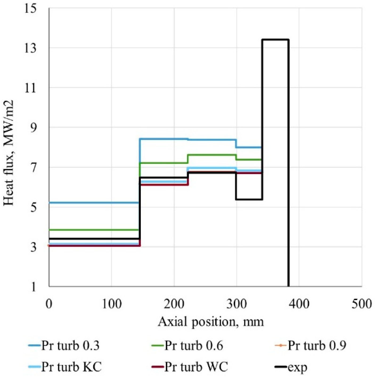
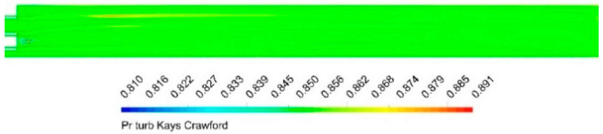
4.3. Turbulent Prandtl Number Effect

The computed average heat flux profile and pressure distribution for three constant turbulent Prandtl values and two algebraic approaches were compared to the measured values. Figure 18 and Figure 19 shows the axial absolute and normalized pressure values for a band of models. During the study, a flamelet model for combustion, the SST turbulence model, and the P1 model with the WSGG spectral approach for radiative heat transfer were used. The unity wall emissivity was set for these simulations. The turbulent Prandtl value mostly affects the normalized lines and the lower the $P{r}_t$, the more concave the profile along the thruster. $P{r}_t$ = 0.9, however, gave quite similar pressure values as the variable turbulent Prandtl models. The segment averaged heat flux profile comparison (Figure 20) also shows some interesting aspects. Heat flux increases with decreasing turbulent Prandtl and the results derived with the constant value of 0.9 were in the vicinity of the heat fluxes obtained with the algebraic variable models. Additional studies showed that this effect remains for cases without radiation modeling and for any turbulence models. The integral HF and radiative-to-total heat flux ratio (RHF/THF) outlined in

Table 3. Influence of the turbulent Prandtl number approach.

Criterion	Turbulent Prandtl Number
	0.3	0.6	0.9	KC	WC	Exp
Integral, MW	0.2247	0.189	0.16248	0.16542	0.1614	0.16
Radiative/Total	0.184	0.198	0.208	0.208	0.209	-

indicate this dependence; another interesting thing is that the RHF fraction increases with increasing $P{r}_t$ and at the level of 0.9, it is the same as for the algebraic $P{r}_t$ models. The increasing tendency is easily explained by the change of the convective heat flux fraction due to Prandtl increase, whereas the similarity of the $P{r}_t$ value of 0.9 with the algebraic locally variable approaches showed that this value (and values in the vicinity) is dominant in the studied thruster. These values also give the best fit for the test measurements.

This was proved by turbulent Prandtl fields for the Kays and Crawford and Wassel and Catton formulations (Figure 21 and Figure 22). The KC model gives the turbulent Prandtl range of 0.84–0.89 while the WC Prandtl number varied from 0.87 to 0.94. In general, these results correlate with the approximations taken by other authors [3,4,5,6,7,8] and show that the assumptions to take values in the range of 0.85–0.9 were valid. However, the variable models had large advantages over the constant values approaches—these are universal for a vast variety of injection schemes and are still robust—there had been no convergence difficulties or slowdown during simulations. Therefore, both KC and WC approaches can be recommended for engineering implementation and for future advanced research.

4.4. Turbulence Modeling Study

The study of turbulence model influence was done with the following modeling approaches fixed for all calculations: a flamelet combustion model, a default turbulent Prandtl number (0.9) to minimize the possible convergence issues, and radiation was neglected in these simulations. The three turbulence models studied were the $k–\omega$ SST, a $k–\epsilon$, and the BSL EARSM model to account for turbulence anisotropy. The SST and BSL EARSM used a default automatic wall treatment approach that is based on a switch between the low-Reynolds and high-Reynolds modeling, while the $k–\epsilon$ model applied a default scalable wall function [33]. However, as it above-mentioned, in this case, the first grid node was intentionally located in the logarithmic sublayer, therefore all models used a default wall function approach implemented in CFX. Initially, the k–ω based BaseLine Reynolds stress model (BSL RSM) and the $k–\epsilon$ based Speziale–Sarkar–Gatski (SSG) Reynolds stress models were also planned to be studied, but the SSG model showed highly unstable convergence behavior and made it challenging to get the converged data in a reasonable amount of time. The BSL RSM simulations, in contrast, converged smoothly but resulted in one order of magnitude unphysically higher eddy viscosity for the central injector, which had not been noticed for other turbulence models (even for the partially converged SSG case). The cause of this is still under investigation, but the probable reason is the symmetry boundary conditions for the 1/6 sector of the central injector or ambiguity in the turbulence boundary conditions. In future, periodic boundary conditions should be applied and a study of boundary conditions should be planned to explore this behavior.

The normalized pressure profiles (Figure 23) showed a better prediction of the pressure peak in the first 100 mm after the injector by the SST model. The $k–\epsilon$ and BSL EARSM models similarly calculated the absolute pressure, whereas the SST model gave 0.2 bar less pressure on average. This behavior correlates with the results of other authors [3,4,5,6,7,8] as the $k–\epsilon$ types of models usually showed better mixing and higher pressures. Here, this effect was also addressed by the higher eddy viscosity given by the $k–\epsilon$ model and thus more intensive mixing. The BSL EARSM model showed even higher eddy viscosities in the near-injector region and in the back of the cylindrical part, which resulted in augmented pressure in these areas. The BSL EARSM gave higher heat fluxes in the first segment and slightly fewer values in the middle. The heat production by the SST model was the smallest among all described models (Figure 24, Figure 25, Figure 26, Figure 27 and Figure 28). Giving both more convenient results for the pressure and quite a nice fit for the heat flux among other models, the BSL EARSM model was recommended for further use.

4.5. General Considerations

As was shown above, the BSL EARSM for turbulence and adiabatic flamelet for combustion performed best among the studied approaches. In this section, these models were combined with the P1 WSGG radiative transport and Wassel–Catton model for $P{r}_t$. However, the amount of radiative heat flux impinged on walls can be very sensitive to the absorption and emission. This because during a firing test, the initial emissivity of the wall surface is not exactly known and may change along both the axis and in time due to varying temperatures and the formation of oxides, so is a source of ambiguity in the RHF estimation. Therefore, a sensitivity study for three values of wall emissivity was provided of ε = 0.1, 0.5, and 1. The results of the described cases coupled with the non-radiating simulations are presented below (Figure 29, Figure 30 and Figure 31) and in

Table 4. Influence of radiation and wall emissivity.

Criterion	Wall Emissivity
	0.1	0.5	1	No Radiation	Exp
Integral, MW	0.1494	0.159060	0.177240	0.144780	0.16
Radiative/Total	0.0187	0.077	0.174	---	---

.

Again, radiation introduced no changes to normalized pressures. However, the RHF inclusion with ε = 1 lowered absolute pressures by around 0.3 bar, which also resulted in higher average and integral heat flux compared to the convective case. Due to a lower amount of energy absorbed by the wall when ε= 0.1 and ε= 0.5, those cases gave slightly higher pressures. The ε = 1 radiating case overestimated heat fluxes in the third and fourth segments, while the results also showed the high influence of the emissivity on wall RHF. The best fit with the experiment, both for the distribution and the integral values were given by ε = 0.5, which gave a RHF/THF ratio of about 7.7%. This value also correlated to estimations given by Thellmann [20] for the ${\mathrm{CH}}_4-{\mathrm{O}}_2$ case. It should be noted again that the real value of emissivity is not known, and even for the known wall material, emissivity varied widely depending on the oxide formation, which is a function of temperature, composition, and therefore axial and tangential position. Thus, only sensitivity reproducing values could be taken and additional studies are needed to establish the true values. However, it can be drawn that the WSGG spectral approach still gives more physical values than the Gray model. All simulations overestimated the experimentally determined values in the fourth segment. Perakis et al. [6] showed that for the fourth and the nozzle segments, the experimental heat flux estimation had discrepancies between the coupled heat transfer calculations and the calorimetric method. This was attributed to a small deficiency of the experimental estimation. The overestimated heat flux values in the first, second, and third segments, however, were due to numerical errors in the present study. Overall, application of the BSL EARSM turbulence model and inclusion of the WSGG model with the average value of ε = 0.5 gave the best representation of the test results among the presented simulations.

During the numerical study, it was found that the applied eddy-viscosity based locally variable turbulent Prandtl models showed similar average values for the Kays and Crawford the turbulent Prandtl varied in the vicinity of 0.84–0.89, whereas for the Wassel and Catton, it was between 0.87–0.93. These values and the behavior of the results given were also close to those derived using the constant $P{r}_t$ 0.9. This corresponds to the approximations of other studies [3,4,5,6,7,8] and is considered to have a good fit with the experimental data. As already mentioned, the BSL EARSM showed the most physical behavior in the near-injector region and best agreement with the test data both for the pressures and the heat flux. This can be attributed to the nonlinear term present in the definition of the turbulent stresses, and therefore better representation of anisotropy in the near-wall and mixing areas. This is a question for further research and comparison with some other RSM models in the future. The k–ω shear-stress transport and k–ε models showed behavior similar to other studies [3,4,5,6,7,8], where the SST model provided less mixing intensity and therefore lower pressures.

The flamelet combustion model was both good at the representation of the pressure fields and the heat fluxes and gave robust and fast performance compared to the enhanced eddy-dissipation method used. The enhanced global reaction eddy-dissipation model gave an error of 8% in pressure, which is acceptable for first engineering estimations, but is still too coarse for the detailed design of a combustor.

The study also showed an overestimation of heat flux using the Gray spectral approximation. This can be improved by the application of the WSGG type of spectral approaches such as the one used in this study. The implementation of the four-gases WSGG approach with wall emissivity equal to unity gave a radiative/total heat flux ratio of about 17–20%, which is more reasonable than the 30% provided by the Gray approach. The wall emissivity average value showed high influence on the wall RHF, whereas the pressure distributions differed insignificantly. Although the used WSGG needs further verification studies and perhaps the inclusion of more gray gases to reproduce thin effects, it can be recommended for rocket propulsion coupled with at least approximate data for the wall emissivity coefficients.

Although some exact recommendations for the use of numerical models of the particular physical phenomena can be given as a result of the current study, additional research is needed to generalize the model choice for different environments (e.g., different mass flows or geometry). However, using the variable turbulent Prandtl approximations studied can be a source for generalization compared to the constant turbulent Prandtl as they include the effect of turbulent viscosity, which is a flow property, and originating from a turbulence model, is defined mostly by the geometry and injection parameters. The combined behavior of the turbulence models and the turbulent Prandtl approaches is anyway a point for further research.

It should also be especially mentioned that during the study, some results of previously observed papers were reaffirmed. For example, the difference between the numerical and experimental absolute pressures about 0.8 bar corresponded to the results presented by authors in other research papers [3,4,5,6,7,8] with differences varying from 0.4–1 bar approximately. Additionally, the comparative behavior of the k–epsilon and k–omega SST models showed similar performance concerning the pressure fields and species stratification. Furthermore, the influence of the turbulent Prandtl on the flowfield and resulting pressure and HF distributions was also as high as some other propulsion study papers have shown [13,14,15,16,17,18,19]. There were also differences compared to the mentioned papers, for example, the resulting absolute pressures for the k–epsilon and SST models were lower than those outlined by Perakis et al. [6,7]. This can be attributed to the wall function approach used in our study compared to the full boundary-layer resolving approach presented in this paper and to other minor differences between the setups. This outcome needs further extensive study.

In general, the results presented in the paper can contributed to the design and optimization of rocket propulsion devices in different ways. First, the exploration of the BSL EARSM (which keeps being a preferable choice compared to common RSM models with regard to calculation resources while still accounting for anisotropy) behavior and its possible performance in other propulsion environment can lower the time demands for the simulations while performing even better than some of the commonly used models studied here. Second, the application of the algebraic variable turbulent Prandtl approaches makes it possible to account for the geometry and injection parameters in the turbulent diffusion phenomena, which is very important for massive datasets of design data on the early design. The effect of radiation on the wall heat flux presented in the paper once again points out the importance of accounting for the radiative transfer in propulsion systems, which is not very resourceful compared to the many different physical phenomena encountered. It also notes that the WSGG type of models combined with the P1 model could be a prospective choice for such applications. All these outcomes can also be useful for everyday routine optimization simulations in the propulsion device design as, at least in the present study, they provide reasonable accuracy coupled with robustness and computational demands corresponding to such objectives.

5. Conclusions

Several 3D Favre-averaged Navier–Stokes simulations of a seven-element rocket thruster operating on GOX/GCH4 were carried out. During these simulations, a comparative study was produced for turbulence and combustion modeling approaches as well as for turbulent Prandtl approximations.

Both the Wassel–Catton and Kays–Crawford turbulent Prandtl approaches provided physical and reasonable results and did not result in any convergence difficulties or high resource requirements and can thus be recommended for future industrial simulations or numerical studies as they are suitable for any injection and mixing types.

The comparison of the combustion simulation methods showed that the adiabatic flamelet libraries generated using the C1 skeletal mechanism are more relevant for the present case than the EDM applied. The implied EDM approach, obviously, can be used for first approximations, but is not applicable for further comprehensive studies. The applied WSGG spectral model showed more reasonable behavior than the Gray model and is suggested for further usage and study. However, a more detailed survey of different WSGG models for methane–oxygen combustion is needed as well as a possible analysis of its performance based on other test cases with at least approximate values of wall emissivity provided from the experiment. Furthermore, usage of different radiation models (e.g., Monte-Carlo or discrete ordinates) with the WSGG type of spectral approach is suggested in future studies of propulsion devices. Another important outcome is the need to include the radiative heat flux in the simulations as the resulting wall heat flux field might be underestimated.

Finally, the combined application of the BSL EARSM, the adiabatic flamelet, the P1 radiation model with the WSGG approach with emissivity ε = 0.5, and the use of algebraic $P{r}_t$ models gave the best approximation of the experimental data. The resulting error in absolute pressures was around 2.9%, and the results for the wall heat flux were also sufficiently similar to the experimental ones, taking into account the discrepancies in the fourth segment. Another important finding of this research is that all these results were obtained on a relatively coarse grid having log-law area $y^{+}$ values, where default wall functions were applied. Though the reliable academic/scientific usage of wall functions combined with RANS algorithms for such applications is an object of further research, the applied and chosen approaches can be used for routine engineering optimization simulations, which would result in reasonable results for the pressures and heat flux parameters. Future work, as suggested, should concentrate on the extensive radiation modeling approaches by studying the turbulence modeling effects as well as more comprehensive analysis of the near-wall resolution influence on the resulting integral parameters.

References

1. Silvestri, S.; Celano, M.P.; Schlieben, G.; Haidn, O.J. Characterization of a Multi-Injector Gox-Gch4 Combustion Chamber. In Proceedings of the 52nd AIAA/SAE/ASEE Joint Propulsion Conference, Salt Lake City, UT, USA, 25–27 July 2016. [Google Scholar]
2. Silvestri, S.; Kirchberger, C.; Schlieben, G.; Celano, M.P.; Haidn, O. Experimental and Numerical Investigation of a Multi-Injector GOX-GCH4 Combustion Chamber. Trans. Jpn. Soc. Aeronaut. Space Sci. Aerosp. Technol. Jpn. 2018, 16, 374–381. [Google Scholar] [CrossRef] [Green Version]
3. Roth, C.M.; Haidn, O.J.; Chemnitz, A.; Sattelmayer, T.; Frank, G.; Müller, H.; Zips, J.; Keller, R.; Gerlinger, P.M.; Maestro, D. Numerical investigation of flow and combustion in a single element GCH4/GOx rocket combustor. In Proceedings of the 52nd AIAA/SAE/ASEE Joint Propulsion Conference, Salt Lake City, UT, USA, 25–27 July 2016; p. 4995. [Google Scholar]
4. Chemnitz, A.; Sattelmayer, T.; Roth, C.; Haidn, O.; Daimon, Y.; Keller, R.; Gerlinger, P.; Zips, J.; Pfitzner, M. Numerical Investigation of Reacting Flow in a Methane Rocket Combustor: Turbulence Modeling. J. Propuls. Power 2018, 34, 864–877. [Google Scholar] [CrossRef]
5. Maestro, D.; Cuenot, B.; Chemnitz, A.; Sattelmayer, T.; Roth, C.; Haidn, O.J.; Daimon, Y.; Keller, R.; Gerlinger, P.M.; Frank, G.; et al. Numerical Investigation of Flow and Combustion in a Single-Element GCH4/GOX Rocket Combustor: Chemistry Modeling and Turbulence-Combustion Interaction. In Proceedings of the 52nd AIAA/SAE/ASEE Joint Propulsion Conference, Salt Lake City, UT, USA, 25–27 July 2016. [Google Scholar] [CrossRef] [Green Version]
6. Perakis, N.; Rahn, D.; Haidn, O.J.; Eiringhaus, D. Heat Transfer and Combustion Simulation of Seven-Element O2/CH4 Rocket Combustor. J. Propuls. Power 2019, 35, 1080–1097. [Google Scholar] [CrossRef]
7. Perakis, N.; Strauß, J.; Haidn, O.J. Heat flux evaluation in a multi-element CH4/O2 rocket combustor using an inverse heat transfer method. Int. J. Heat Mass Transf. 2019, 142, 118425. [Google Scholar] [CrossRef]
8. Perakis, N.; Haidn, O.J.; Eiringhaus, D.; Rahn, D.; Zhang, S.; Daimon, Y.; Karl, S.; Horchler, T. Qualitative and Quantitative Comparison of RANS Simulation Results for a 7-Element GOX/GCH4 Rocket Combustor. In Proceedings of the 54th AIAA/SAE/ASEE Joint Propulsion Conference, Cincinnati, OH, USA, 9–11 July 2018; p. 54. [Google Scholar]
9. Nasuti, F.; Concio, P.; Indelicato, G.; Lapenna, P.E.; Creta, F. Role of Combustion Modeling in the Prediction of Heat Transfer in LRE Thrust Chambers. In Proceedings of the 8th European Conference for Aeronautics and Aerospace Sciences (EUCASS), Madrid, Spain, 1–4 July 2019. [Google Scholar]
10. Zhukov, V.P. Computational Fluid Dynamics Simulations of a GO2/GH2 Single Element Combustor. J. Propuls. Power 2015, 31, 1–8. [Google Scholar] [CrossRef] [Green Version]
11. Zhukov, V.P.; Suslov, D.I. Measurements and modelling of wall heat fluxes in rocket combustion chamber with porous injector head. Aerosp. Sci. Technol. 2016, 48, 67–74. [Google Scholar] [CrossRef]
12. Poschner, M.; Pfitzner, M. Real Gas CFD Simulation of Supercritical H2-LOX in the MASCOTTE Single Injector Combustor Using a Commercial CFD Code. In Proceedings of the 46th AIAA Aerospace Sciences Meeting and Exhibit, Reno, Nevada, 7–10 January 2008; Volume 46. [Google Scholar] [CrossRef]
13. Molchanov, A.M.; Bykov, L.V.; Nikitin, P.V. Modeling High-Speed Reacting Flows with Variable Turbulent Prandtl and Schmidt Numbers. In Proceedings of the 9th International Conference on Heat Transfer, Fluid Mechanics and Thermodynamics, Valletta, Malta, 16–18 July 2012. [Google Scholar]
14. Yimer, I.; Campbell, I.; Jiang, L.-Y. Estimation of the Turbulent Schmidt Number from Experimental Profiles of Axial Velocity and Concentration for High-Reynolds-Number Jet Flows. Can. Aeronaut. Space J. 2002, 48, 195–200. [Google Scholar] [CrossRef]
15. He, G.; Guo, Y.; Hsu, A.T. The effect of Schmidt number on turbulent scalar mixing in a jet-in-crossflow. Int. J. Heat Mass Transf. 1999, 42, 3727–3738. [Google Scholar] [CrossRef]
16. Keistler, P.; Xiao, X.; Hassan, H.; Rodriguez, C. Simulation of Supersonic Combustion Using Variable Turbulent Prandtl/Schmidt Number Formulation. In Proceedings of the 36th AIAA Fluid Dynamics Conference and Exhibit, San Francisco, CA, USA, 5–8 June 2006. [Google Scholar]
17. Ivancic, B.; Riedmann, H.; Frey, M.; Knab, O.; Karl, S.; Hannemann, K. Investigation of Different Modeling Approaches for CFD Simulation of High Pressure Rocket Combustors. In Proceedings of the 5th European Conference for Aerospace Sciences (EUCASS), Munich, Germany, 1–5 July 2013. [Google Scholar]
18. Xiao, X.; Edwards, J.; Hassan, H.; Cutler, A. A Variable Turbulent Schmidt Number Formulation for Scramjet Application. In Proceedings of the 43rd AIAA Aerospace Sciences Meeting and Exhibit, Reno, Nevada, 10–13 January 2005. [Google Scholar] [CrossRef] [Green Version]
19. Goldberg, U.C.; Palaniswamy, S.; Batten, P.; Gupta, V. Variable Turbulent Schmidt and Prandtl Number Modeling. Eng. Appl. Comput. Fluid Mech. 2010, 4, 511–520. [Google Scholar] [CrossRef]
20. Thellmann, A. Impact of Gas Radiation on Viscous Flows, in Particular on Wall Heat Loads, in Hydrogen-Oxygen vs. Methane-Oxygen Systems, Based on the SSME Main Combustion Chamber. Ph.D. Thesis, Universitaet der Bundeswehr, Muenchen, Germany, 2010. [Google Scholar]
21. Leccese, G.; Bianchi, D.; Nasuti, F. Numerical Investigation on Radiative Heat Loads in Liquid Rocket Thrust Chambers. J. Propuls. Power 2019, 35, 930–943. [Google Scholar] [CrossRef]
22. Molchanov, A.M.; Bykov, L.V.; Yanyshev, D.S. Calculating thermal radiation of a vibrational nonequilibrium gas flow using the method of k-distribution. Thermophys. Aeromech. 2017, 24, 399–419. [Google Scholar] [CrossRef]
23. Mazzei, L.; Puggelli, S.; Bertini, D.; Pampaloni, D.; Andreini, A. Modelling soot production and thermal radiation for turbulent diffusion flames. Energy Procedia 2017, 126, 826–833. [Google Scholar] [CrossRef]
24. Poitou, D.; El Hafi, M.; Cuenot, B. Analysis of Radiation Modeling for Turbulent Combustion: Development of a Methodology to Couple Turbulent Combustion and Radiative Heat Transfer in LES. J. Heat Transf. 2011, 133, 062701. [Google Scholar] [CrossRef] [Green Version]
25. Daimon, Y.; Negishi, H.; Silvestri, S.; Haidn, O.J. Conjugated Combustion and Heat Transfer Simulation for a 7 element GOX/GCH4 Rocket Combustor. In Proceedings of the 54th AIAA/SAE/ASEE Joint Propulsion Conference, Cincinnati, OH, USA, 9–11 July 2018; pp. 2018–4553. [Google Scholar]
26. Muto, D.; Daimon, Y.; Shimizu, T.; Negishi, H. Wall modeling of reacting turbulent flow and heat transfer in liquid rocket engines. In Proceedings of the 54th AIAA/SAE/ASEE Joint Propulsion Conference, Cincinnati, OH, USA, 9–11 July 2018. [Google Scholar] [CrossRef]
27. Balaras, E.; Benocci, C.; Piomelli, U. Two-layer approximate boundary conditions for large-eddy simulations. AIAA J. 1996, 34, 1111–1119. [Google Scholar] [CrossRef]
28. Rani, S.L.; Smith, C.E.; Nix, A.C. Boundary-Layer Equation-Based Wall Model for Large-Eddy Simulation of Turbulent Flows with Wall Heat Transfer. Numer. Heat Transfer Part B Fundam. 2009, 55, 91–115. [Google Scholar] [CrossRef]
29. Kawai, S.; Larsson, J. Wall-modeling in large eddy simulation: Length scales, grid resolution, and accuracy. Phys. Fluids 2012, 24, 15105. [Google Scholar] [CrossRef]
30. Piomelli, U. Wall-layer models for large-eddy simulations. Prog. Aerosp. Sci. 2008, 44, 437–446. [Google Scholar] [CrossRef]
31. Larsson, J.; Kawai, S.; Bodart, J.; Bermejo-Moreno, I. Large eddy simulation with modeled wall-stress: Recent progress and future directions. Mech. Eng. Rev. 2016, 3, 1–23. [Google Scholar] [CrossRef] [Green Version]
32. Maheu, N.; Moureau, V.; Domingo, P.; Duchaine, F.; Balarac, G. Large-Eddy Simulations of flow and heat transfer around a low-Mach number turbine blade. Center for Turbulence Research. In Proceedings of the Summer Program, Stanford, CA, USA, 24 June–20 July 2012. [Google Scholar]
33. Ansys. CFX Theory Guide; ANSYS Inc.: Canonsburg, PA, USA, 2019; Volume 15317, p. R2. [Google Scholar]
34. Yoder, D.A. Comparison of Turbulent Thermal Diffusivity and Scalar Variance Models. In Proceedings of the 54th AIAA Aerospace Sciences Meeting, San Diego, CA, USA, 4–8 January 2016; p. 54. [Google Scholar] [CrossRef] [Green Version]
35. Kays, W.M.; Whitelaw, J.H. Convective Heat and Mass Transfer. J. Appl. Mech. 1967, 34, 254. [Google Scholar] [CrossRef]
36. Wassel, A.; Catton, I. Calculation of turbulent boundary layers over flat plates with different phenomenological theories of turbulence and variable turbulent Prandtl number. Int. J. Heat Mass Transf. 1973, 16, 1547–1563. [Google Scholar] [CrossRef]
37. Centeno, F.R.; Da Silva, C.V.; Brittes, R.; França, F.H.R. Numerical simulations of the radiative transfer in a 2D axisymmetric turbulent non-premixed methane–air flame using up-to-date WSGG and gray-gas models. J. Braz. Soc. Mech. Sci. Eng. 2015, 37, 1839–1850. [Google Scholar] [CrossRef]
38. Ansys. Fluent Theory Guide; ANSYS Inc.: Canonsburg, PA, USA, 2019; Volume 15317, p. R2. [Google Scholar]
39. Peters, N. Laminar diffusion flamelet models in non-premixed turbulent combustion. Prog. Energy Combust. Sci. 1984, 10, 319–339. [Google Scholar] [CrossRef]
40. Magnussen, B.; Hjertager, B. On Mathematical Modeling of Turbulent Combustion with Special Emphasis on Soot Formation and Combustion. Symp. (Int.) Combust. Camb. Mass. 1977, 16, 719–729. [Google Scholar] [CrossRef]
41. Rocket Propulsion Analysis, Version 2.3 User Manual. Cologne, Germany. 2017. Available online: http://www.propulsion-analysis.com/ (accessed on 5 April 2020).
Figure 1. View of the studied thrust chamber [1,2].
Energies 13 05009 g001
Figure 2. Domain and boundary conditions.
Energies 13 05009 g002
Figure 3. Axial wall temperature profile [1,2].
Energies 13 05009 g003
Figure 4. Mesh front view.
Energies 13 05009 g004
Figure 5. Pressure axial distribution.
Energies 13 05009 g005
Figure 6. Normalized axial pressure distribution.
Energies 13 05009 g006
Figure 7. Segment averaged heat flux density distribution.
Energies 13 05009 g007
Figure 8. Normalized axial pressure distribution.
Energies 13 05009 g008
Figure 9. Absolute pressure axial distribution.
Energies 13 05009 g009
Figure 10. Segment average heat flux distribution.
Energies 13 05009 g010
Figure 11. The no-radiating temperature field (50% axial scaling).
Energies 13 05009 g011
Figure 12. The P1 Gray model temperature field (50% axial scaling).
Energies 13 05009 g012
Figure 13. The P1 WSGG model temperature field (50% axial scaling).
Energies 13 05009 g013
Figure 14. The Gray model radiation intensity (50% axial scaling).
Energies 13 05009 g014
Figure 15. The WSGG model radiation intensity (50% axial scaling).
Energies 13 05009 g015
Figure 16. The H 2 O mass fraction field (50% axial scaling).
Energies 13 05009 g016
Figure 17. The CO 2 mass fraction field (50% axial scaling).
Energies 13 05009 g017
Figure 18. Axial normalized pressure.
Energies 13 05009 g018
Figure 19. Absolute pressure axial distribution.
Energies 13 05009 g019
Figure 20. Segment averaged heat flux distribution.
Energies 13 05009 g020
Figure 21. P r t field in the cylindrical part given by the Kays and Crawford model.
Energies 13 05009 g021
Figure 22. P r t field in the cylindrical part given by the Wassel and Catton model.
Energies 13 05009 g022
Figure 23. Normalized axial pressure distribution.
Energies 13 05009 g023
Figure 24. Absolute pressure distribution.
Energies 13 05009 g024
Figure 25. Segment averaged heat flux distribution.
Energies 13 05009 g025
Figure 26. k ε model eddy viscosity distribution (50% axial scaling).
Energies 13 05009 g026
Figure 27. SST model eddy viscosity distribution (50% axial scaling).
Energies 13 05009 g027
Figure 28. BSL EARSM model eddy viscosity distribution (50% axial scaling).
Energies 13 05009 g028
Figure 29. Normalized axial pressure distribution.
Energies 13 05009 g029
Figure 30. Pressure axial distribution.
Energies 13 05009 g030
Figure 31. Segment average heat flux distribution.
Energies 13 05009 g031