Abstract
The purpose of this work is modeling of a horizontal oil–water flow with and without the Algebraic Interfacial Area Density (AIAD) model. Software and hardware developments in the past years have significantly increased and improved the accuracy, flexibility, and performance of simulations for large and complex problems typically encountered in industrial applications. At Helmholtz-Zentrum Dresden-Rossendorf (HZDR), the focus has been concentrated on the R&D of new modeling capabilities for Euler–Euler approach where interfaces exist. In this research paper, the applicability of the AIAD model for a horizontal oil–water flow is investigated. The comparison between the standard ANSYS Fluent Eulerian Interface Capabilities (namely Multi-Fluid VOF) without AIAD and ANSYS CFX with AIAD implemented via user functions for the oil–water flow was performed. Thereafter, the obtained results were compared with existing experimental data produced by the Department of Thermodynamics and Transport Phenomena of the University Simon Bolivar (USB) in Caracas, Venezuela. The results of the simulations show that horizontal oil–water flow can be modelled with rather acceptable accuracy when using regime transition capabilities as those offered by the AIAD model.
1. Introduction
Multi-phase flows occur in various industrial applications, such as in the petrochemical industry, process engineering, and in the energy industry. In order to improve the quality of these products and to achieve the highest possible safety in these industries, the further development and optimization of novel calculation methods for multiphase flow is of great importance but also presents a great challenge.
In the petrochemical industry, oil–water flows in horizontal pipelines are relevant. In order to increase the lifetime of the pipe system and to improve and optimize the flow characteristics, the behavior of the flow must be predicted.
During the co-current flow of oil and water in pipes, the deformable interface of the two fluids can attain a variety of characteristic configurations known as flow regimes. Accurate prediction of oil–water flow characteristics such as the flow regime, water holdup, and pressure gradient are very important for engineering design and operation. This requires better modeling and predictability of the interfacial forces. In the further development and optimization of new calculation methods for multiphase flow, increasingly numerical methods of fluid mechanics are used. An exact knowledge of the occurring flow phenomena is necessary. The use of Computational Fluid Dynamics (CFD) offers three major advantages: reduction of development time, reduction of costs, and increase in flexibility. The experimental investigations of the flow of two liquid phases are complicated. The production of the samples and the measuring methods used are very expensive. The aim of the work is to investigate the applicability of the Algebraic Interfacial Area Density (AIAD) model [1] using ANSYS CFX for an oil–water multicomponent flow. We further compare the CFX results to the inherent Eulerian free-surface approach offered in Fluent and known as Multi-Fluid VOF without AIAD. For these purposes, various calculations are performed at different oil and water inlet velocities and various boundary conditions that are based on experimental data. The main objective of this work is to compare the qualitative results obtained by ANSYS CFX and Fluent with existing experimental data of an oil–water flow in a horizontal pipe. This refers to the distribution of oil volume fraction and interpenetration of both phases along the considered horizontal pipe.
To investigate the effectivity of various turbulence models in simulating two-phase pipeline flow only few studies have been conducted. Walvekar et al. [2] used Fluent to simulated dispersed oil–water horizontal pipeline flow. The Eulerian–Eulerian method and the standard k-ε turbulence model was utilized. The predicted results were satisfactory at high mixture velocity, while at low mixture velocity, the authors observed notable discrepancy to the data. Burlutskiy and Turangan [3] investigated dispersed oil in water in a vertical pipe using a steady Euler–Lagrange model and a k-ε turbulence model implemented in Fluent. The predictions for pressure drop were reasonable at high mixture velocity, and the authors highlighted the importance of the shear-lift force on their prediction.
Shi et al. [4] showed a simulation of horizontal oil–water flow with matched density and medium viscosity ratio (=18.8) in several different flow regimes (core annular flow, oil plugs/bubbles in water and dispersed flow) using Fluent. Satisfactory agreement in the prediction of flow patterns were obtained for core annular flow and oil plugs/bubbles in water. The simulation results also demonstrated some detailed flow characteristics of core annular flow with relatively low-viscosity oil. Different from the velocity profiles of high-viscosity oil core annular flow, where there is sharp change in the velocity gradient at the phase interface with velocity across the oil core being roughly flat, in this case there is no sharp change in the velocity gradient at the phase interface for core annular flow with relatively low-viscosity oil.
Burlutskiy [3] developed a 3D mathematical model of dispersed oil-in-water pipe flow. The model was validated against experiments on frictional pressure drop. The numerical analysis of oil-in-water flow in horizontal pipes was performed. They found that the shear-lift force has much higher importance for the adequate flow representation as compared to the break-up/coalescence phenomena in the case of highly turbulent liquid–liquid dispersed pipe flows.
2. Flow Pattern of the Oil–Water Flow in the Horizontal Pipe
Since each flow path has unique hydrodynamic flow characteristics, it is important to study the different flow patterns in liquid–liquid systems.
To study the flow patterns in microchannels, two main flow morphologies are noticed [5]:
- Segregated flow: in which the two phases flow continuously and separated by gravity or pressure, with the denser on flowing at the bottom.
- Dispersed flow: in which one phase flows continuously while the other phase passes through the continuous one.
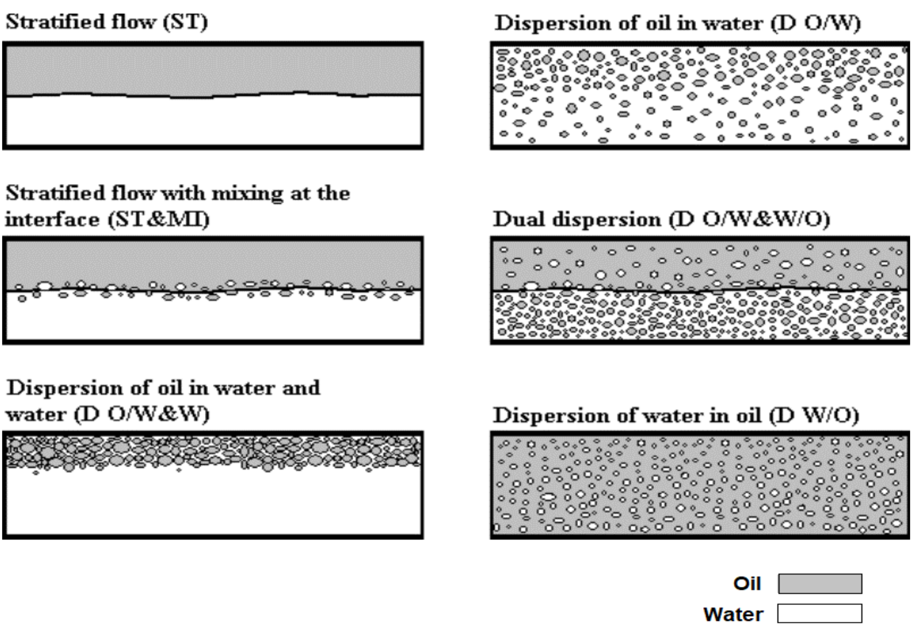
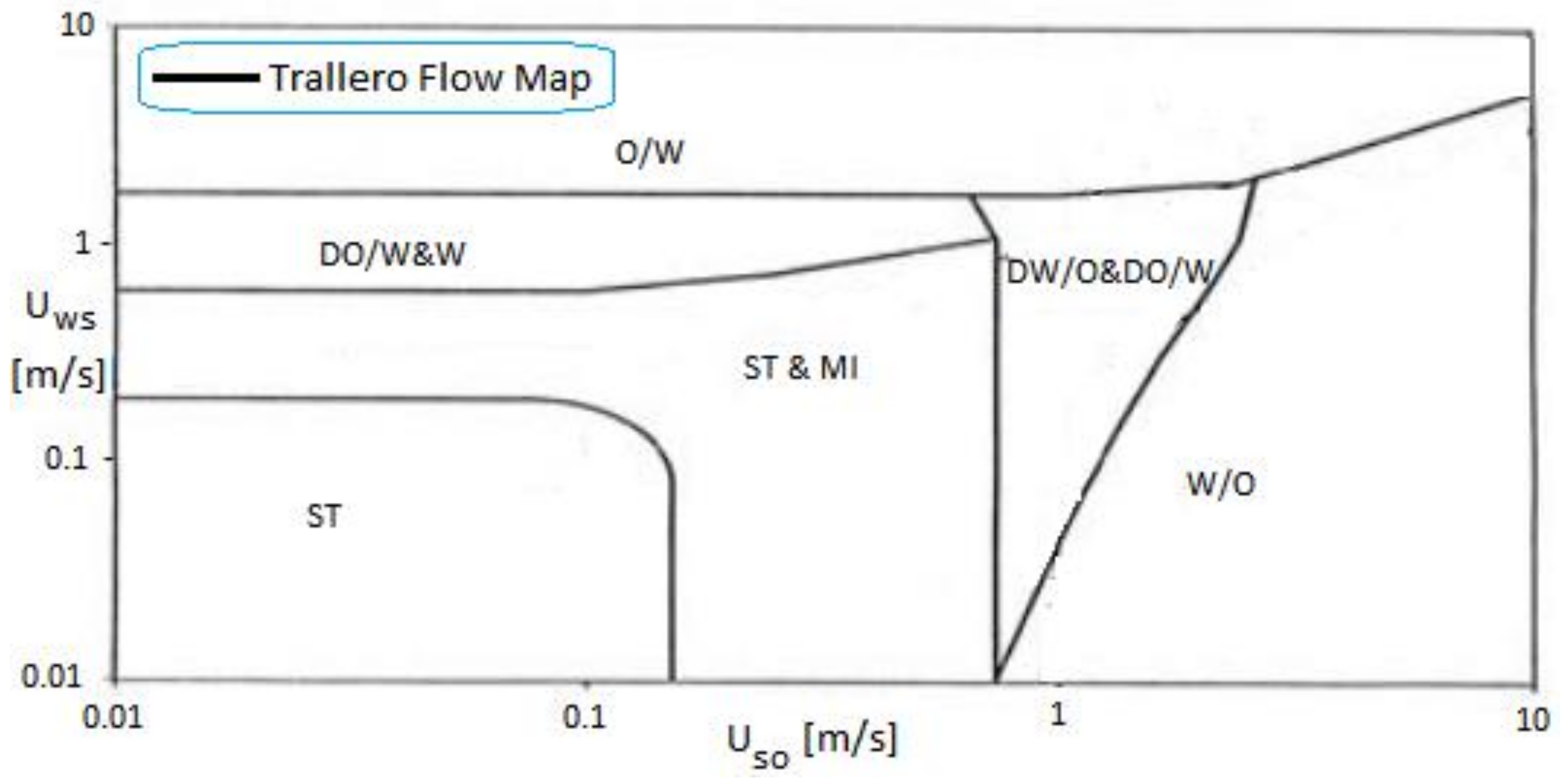
More relevant for this work are the flow patterns studied by Trallero et al. [6]. He encapsulated these into six flow curves as described below (Figure 1):
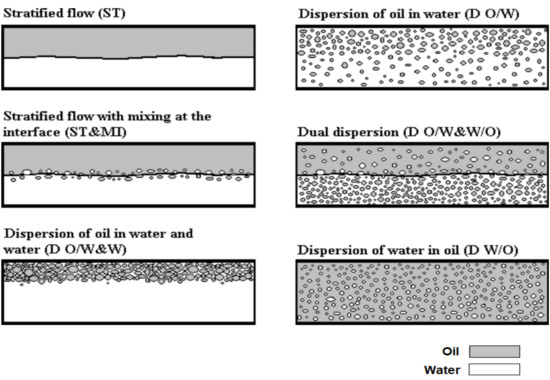
Figure 1.
Flow pattern according to Trallero [6].
- Stratified Flow (ST): The two phases flow separately (the heavier flow at the bottom of the tube) with a smooth interface between the phases.
- Stratified Flow with Mixing at the Interface (ST & MI): In this case the flow is stratified, but the instability of the interface creates a mixing zone. Despite this mixing zone you can see pure liquids at the top and bottom of the tube.
- Dispersion of oil in water and water (DO/W & W): The water is distributed throughout the pipe. While oil droplets flow into the water at the top of the pipe, a pure layer of water flows down the bottom of the pipe.
- Oil in Water Emulsion (O/W): The entire pipe cross-sectional area is occupied by water containing dispersed oil droplets.
- Dispersion of water in oil and oil in water (DO/W & DW/O): The oil is distributed over the entire tube. At the upper side of the tube, water droplets flow in the oil, while at the bottom of the tube oil droplets flow into water.
- Water in Oil Emulsion (W/O): Oil is the dominant phase containing dispersed water droplets.
Figure 2 shows the flow pattern map developed by Trallero et al. [6], which can determine the transition between the patterns according to the relation between the axial surface velocities of water (Uws) and oil (Uso).

Figure 2.
Flow pattern diagram according to Trallero [6].
In the paper of Torres et al. [7] a comprehensive overview of existing experimental oil–water flow studies in horizontal pipelines is presented.
They introduced a new flow pattern transition prediction models for oil–water flow in horizontal pipes. The transition between stratified and non-stratified flow is predicted using Kelvin–Helmholtz (KH) stability analysis for long waves. Additional models are proposed for the prediction of the transition boundaries to semi-dispersed and to fully dispersed flow.
3. Description of the Experiment
The experimental data was produced and postprocessed by the Thermodynamic and Transport Phenomena Department of the University Simon Bolivar (USB) in Caracas, Venezuela [8,9,10,11].
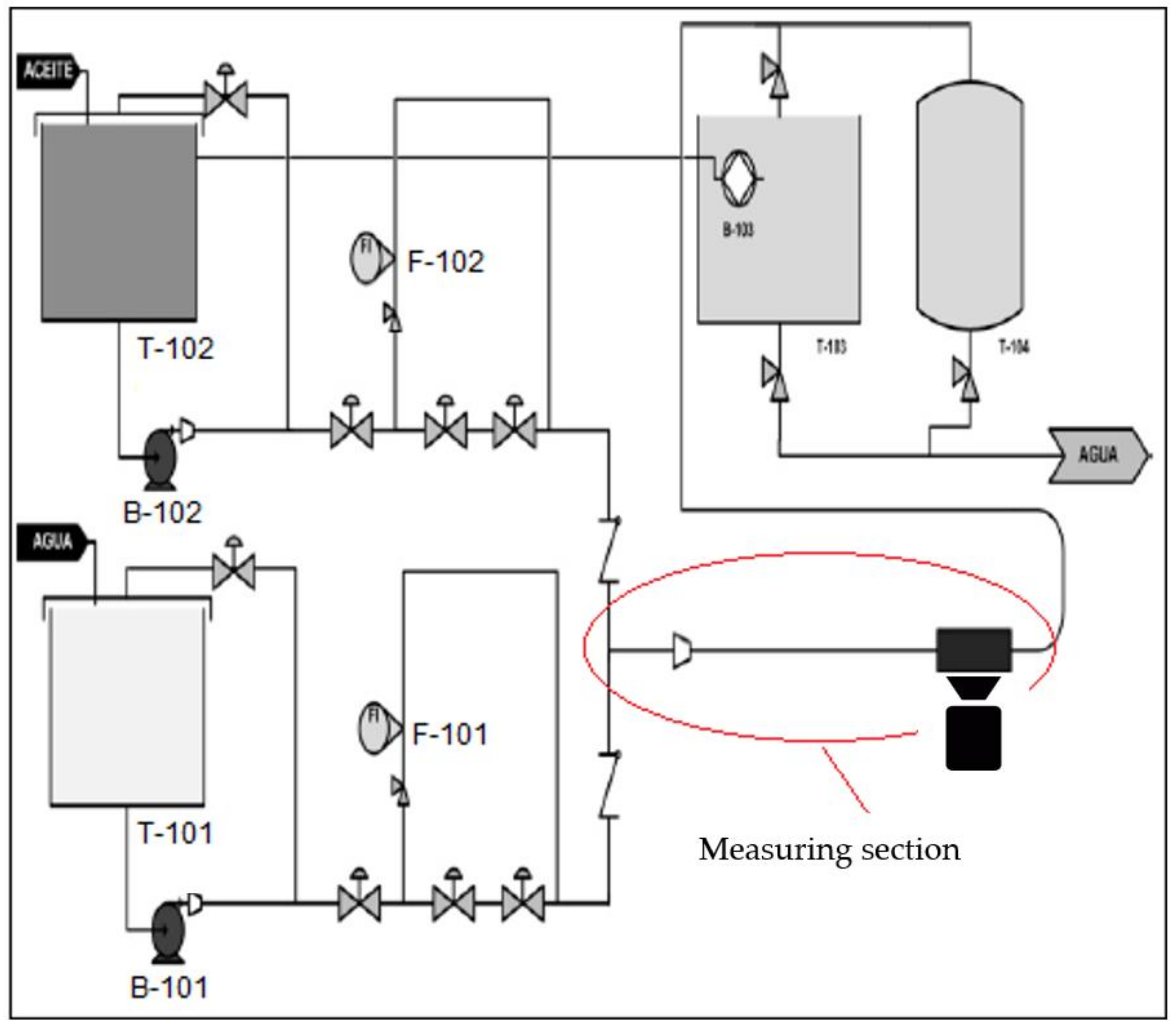
The equipment used to obtain the experimental data consists of three units [9] (Figure 3):

Figure 3.
Setup of experiment [11].
- Infeed unit: water collection tank (T-101), oil sump tank (T-102), two progressing cavity pumps (B-101 and B-102) and two rotameters (FI-101 and FI-102).
- Measuring section: Plexiglas tube with an inner diameter of 0.0445 m (1.75 in) and outer diameter of 0.0508 m (2 in).
- Measurement technology: 4540 mx high-speed camera, which allows shooting from 30 to 4500 frames per second in full-screen mode.
The experimental scheme is divided into three stages [9]:
- Phase Pumping: In this stage, oil and water are pumped to the pipes from the tanks using submerged pumps. The oil and water are mixed in a T-section and move together until reaching the visualization cell in a fully developed stage.
- Visualization: This stage is done using a rectangular cell full of glycerin (in order to improve light conditions, which produced higher quality data and made post-processing easier). Images are taken with a high-speed camera.
- Separation: Finally, the two phases are separated, cleaned, and filtered.
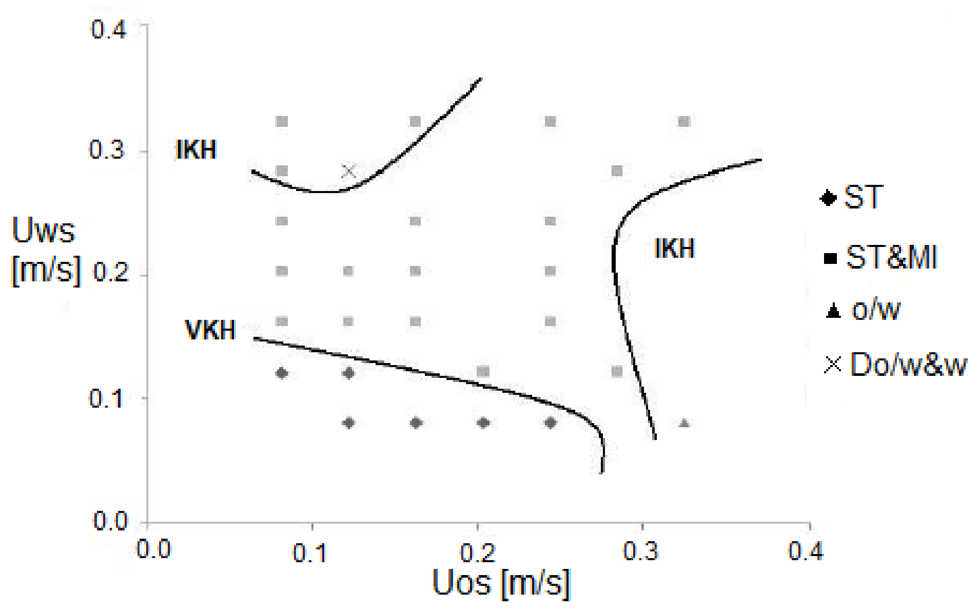
The experimental matrix consists of a very large number of different oil and water velocity cases. A graphical representation was drawn up and is shown in Figure 4.
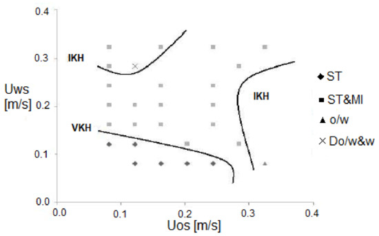
Figure 4.
Flow map of the experiments [11].
In the map (Figure 4) presented by Trallero et al. [6] it can be noted that the stratified flow pattern is defined by the VKH (viscous Kelvin–Helmholtz instability line resulting from the stability analysis of the biphasic mix, which indicates the region where droplet formation begins). As it increases the phase velocity, it can be observed in the diagram that the two inviscid Kelvin–Helmholtz (IKH) instability lines separate the segregated flow patterns from dispersed flow patterns. In the flow map obtained from experimental data, we can distinguish the areas enclosed by the IKH and VKH lines [11].
Four experimental test cases (Figure 5, Figure 6, Figure 7, Figure 8, Figure 9, Figure 10 and Figure 11) were selected with different inlet velocities of oil and water, which are shown in Table 1.
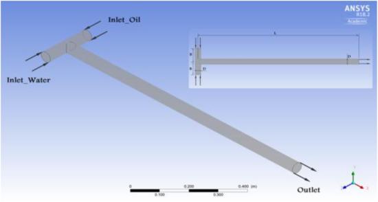
Figure 5.
3D geometry.
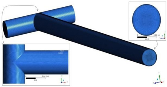
Figure 6.
O-grid discretized grid.
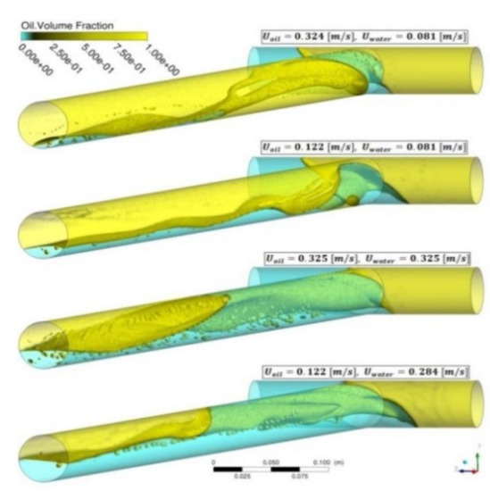
Figure 7.
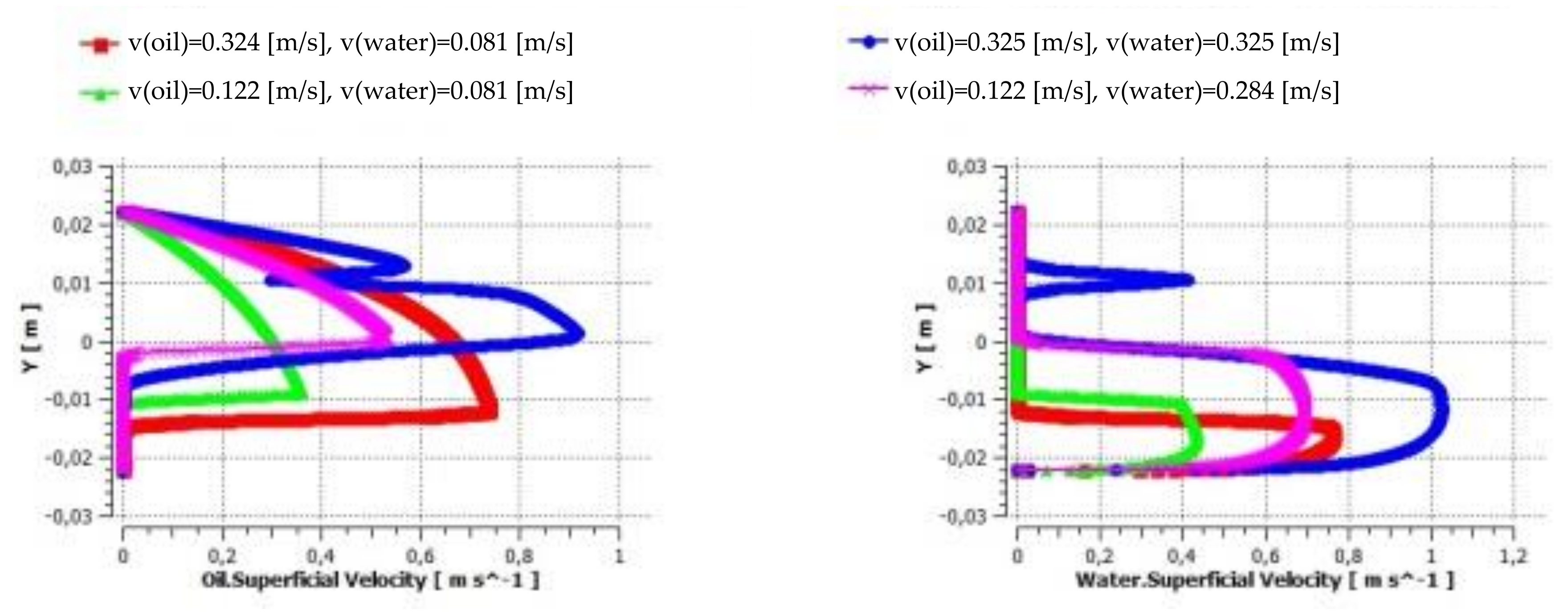
Iso-area of the volume fraction of oil in the whole domain at different inlet velocities of oil and water.
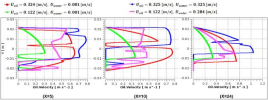
Figure 8.
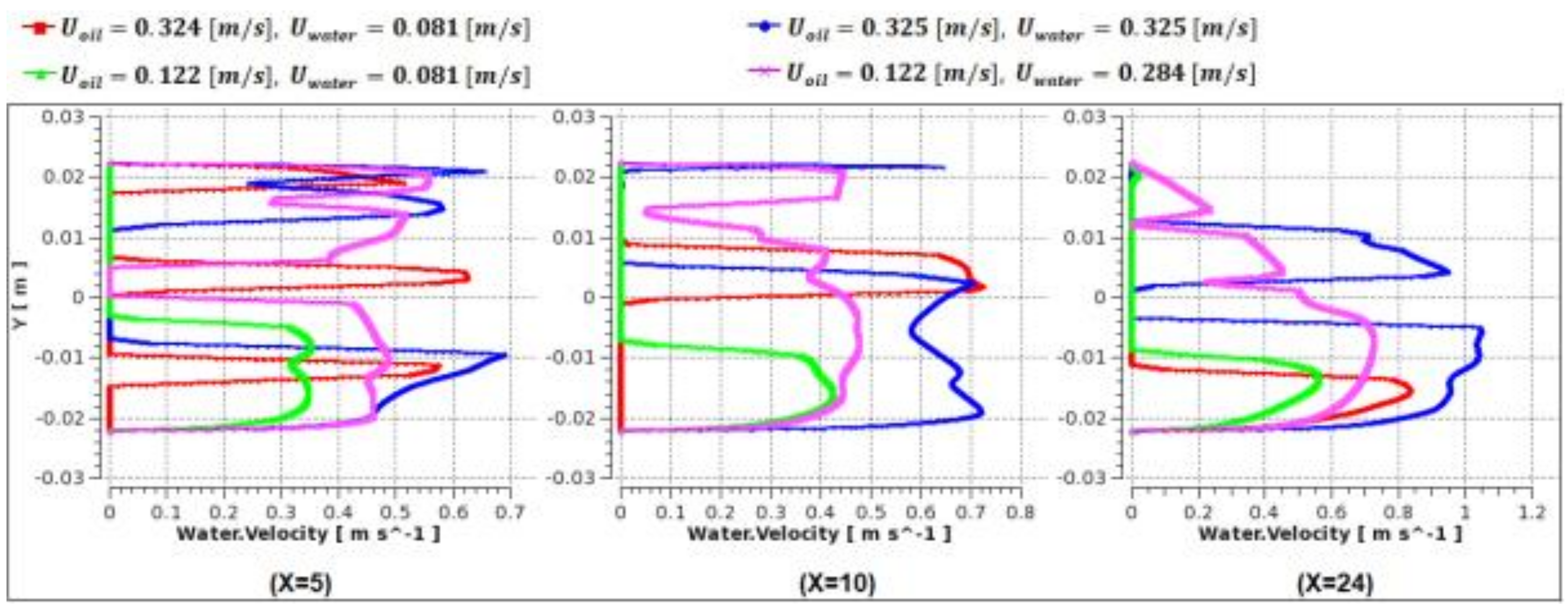
Course of the oil velocity along the vertical line in the Y direction at z = 0 and different dimensionless distances of x = L/D.

Figure 9.
Variation of the water velocity along the vertical line in the Y direction at z = 0 and various dimensionless distances of x = L/D.
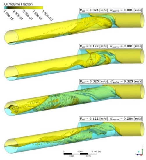
Figure 10.
Oil volume fraction and isosurface of the oil throughout the domain at different oil and water entry velocities.

Figure 11.
The course of the oil and water velocities along the vertical line in the Y direction at z = 0 and x = L/D = 24.

Table 1.
Experiments.
4. The Algebraic Interfacial Area Density Model (AIAD)
The AIAD model allows the recognition of the flow morphology and the consistent switching of arbitrary closure relations. It has already been described by Höhne et al. [12], so only a brief description is given here.
To account for the different flow morphologies, the AIAD model uses blending functions depending on the volume fraction that enable switching between closure laws for dispersed water droplets, dispersed oil droplets and the interfacial flow. Based on these blending functions, different equations for the interfacial area density and the drag coefficient can be applied according to the local morphology. The blending functions are defined as Equations (1) and (2) for water droplet and oil droplet region, respectively and Equation (3) for the interface.
With and being the blending coefficients for water droplets and oil droplets, respectively and , are the critical volume fractions for the water droplet and oil droplet regimes, respectively. In the simulations presented here, values of and were used. For all model coefficients, same values were used as in previous studies [13]. They were chosen independent of the actual geometry and flow regime and no tuning of the AIAD model was done for the work presented here. The threshold value is a critical volume fraction before the coalescence rate increases sharply and is verified by experiments in both vertical and horizontal flows. Published data agree that bubbly flow rarely exceeds a volume fraction of about 0.25–0.35 when the transition to resolved structures occurs [14,15,16]. Parameter studies also indicated that the model is not very sensitive toward a change of the blending function parameters.
For simplicity, oil droplets and water droplets are for now assumed to be of spherical shape, with a constant diameter of and , respectively. Non-drag forces in the regions of dispersed flow are neglected here but can be included if required. The interfacial area density (IAD) in the water droplet regime is given by:
in which is the volume fraction of the water phase. The IAD for oil droplets, , is formulated in an analogous manner. The IAD of the interface, , is defined as the magnitude of the gradient of the water volume fraction
with being the normal direction to the interface. The morphology dependent interfacial area density is then calculated as the sum of , weighted by the blending functions :
5. Modelling the Interfacial Drag
In the general case of a two-phase flow, there is a velocity difference between the fluids, which is commonly called slip velocity. In contrast to volume of fluid (VOF) methods, where only one velocity field is present, within the multi-fluid framework each phase has its own velocity and turbulence field. Therefore, a closure model for the momentum exchange at the phase boundary due to drag is required. The drag force can be correlated with the slip velocity , the fluid density , the surface area and the dimensionless drag coefficient . For geometry-independent modeling the drag force is expressed as the volumetric force density and is then replaced by the interfacial area density . The magnitude of the drag force density is given by Equation (7).
For a dispersed flow, the density of the continuous phase is used in Equation (7). In case of an interface the phase averaged density is used, i.e.,
with and being the density of the oil and the water, respectively.
In simulations of interfacial flows, Equation (7) does not represent a realistic physical model. It is reasonable to expect that the velocities of both fluids in the vicinity of the interface are rather similar. In [13], it is assumed that the shear stress near the interface behaves like a wall shear stress on both sides of the interface in order to reduce the velocity differences of both phases. It is supposed that the morphology region “interface” is acting like a wall and a wall-like shear stress is introduced at the interface, which influences the liquid–liquid momentum transfer. The components of the unit normal vector at the interface are taken from the gradients of the volume fraction.
From theory, shear stress is a symmetric tensor
If we have a surface normal vector then the wall-like interface shear stress vector is the product of the viscous stress tensor and the surface normal vector:
This results in the following equations:
It can also be written as:
It is assumed that the drag force is equal to the wall shear stress force acting at the interface in the vicinity of the interface:
As a result of Equation (14), the modified drag coefficient is dependent on the viscosities of both phases, the wall-like shear stresses (local gradients of liquid/liquid velocities normal to the interface), the mixture density, and the slip velocity between the phases:
The AIAD model uses the following three different drag coefficients: CD,OD = 0.44 (Newton) for oil droplets, CD,WD = 0.44 for the water droplets, and CD,I according to Equation (15) [13] for the interface. More sophisticated drag models for the dispersed regimes can be applied if necessary.
The simulations are based on the Euler–Euler two-fluid framework with the AIAD model as described above. Turbulent stresses are accounted for using the two-equation k-ω-based Shear Stress Turbulence (SST) model according to [17], which is applied to each phase separately. An important goal of the description of two-phase flows is the correct determination of turbulence parameters. These have, for example, a decisive influence on the generation of interface instabilities. Without special treatment of the interface resulting from the use of two-equation turbulence models, the high velocity of the lighter phase particularly leads to higher turbulence at the oil/water interface. In the AIAD approach, the calculation of the turbulence now is done separately for each phase of the k-ω-based SST turbulence model. An additional function similar to the wall damping function for the turbulent diffusion is introduced on the oil/water interface.
Phase-averaged CFD methods, such as the two-fluid model, usually neglect waves below the grid size. Such waves may be formed for instance by Kelvin–Helmholtz instabilities. Despite that, the effect of these sub-grid size waves on liquid side turbulence kinetic energy (TKE) can be noticeably large. Brocchini and Peregrine [18] performed a detailed analysis of strong turbulence at air–water free surfaces which is followed here. The behavior of a gas–liquid interface depends both on gravity and surface tension forces, it can therefore be characterized by the corresponding dimensionless groups, i.e., the turbulent Froude number and the Weber number . Here, represents a turbulent velocity scale, is a turbulent length scale, and σ denotes the interfacial tension coefficient. The effect of sub-grid size waves is considered in terms of a critical Fr, We parameter space where the surface is no longer smooth and does not break up completely. A corresponding volumetric source term for the sub-grid wave turbulence was formulated and added to the liquid side TKE transport equation [1].
6. Numerical Simulations
6.1. Geometry
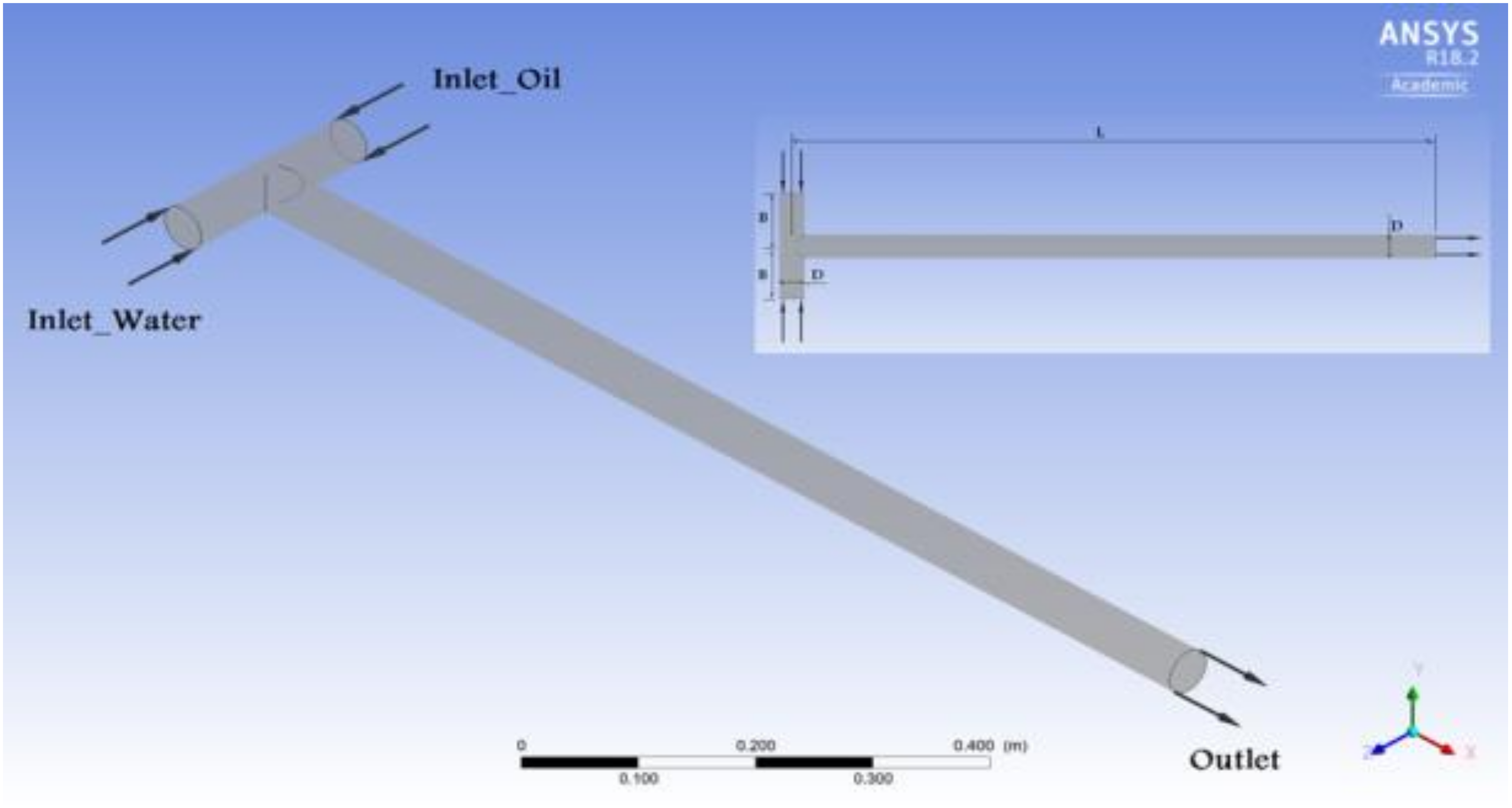
The geometry consists of two horizontal tubes (T-section), which are vertically coupled to each other and have the same diameter (D = 0.0445 m) (Figure 5). The length of both the tubes is 11·D. The oil and the water flow enter the system separately and meet at the t-section.
The geometry was modeled following the experiment (Figure 3). In the simulation, the flow of both fluids develops properly before they are mixed together.
Figure 5 shows the geometry and dimension of the fluid domain:
6.2. Grid Generation
A grid study was performed based on experiences with similar pipes/channels for horizontal two-phase flow modelling [1,12] and the proper mesh resolution was selected. The mesh is based on a block-structured hexahedral grid (O-Grid) generated by ICEM CFD to give accurate results as well as to achieve the convergence of the solution as quickly as possible. The settings of the grid are shown in the following Table 2 and Figure 6.
Table 2.
Grid settings.
6.3. Input Deck
After generating the volume mesh, the models were run using ANSYS CFX with AIAD and ANSYS FLUENT without AIAD.
6.3.1. Fluent-Solver
Fluent software (FLUENT 2018 R3) contains a broad number of physical multiphase modeling capabilities needed to simulate flow, turbulence, heat transfer, and reactions for industrial applications.
Nevertheless, until FLUENT 2019 R3, this solver did not include any regime transition capabilities such as AIAD. Therefore, this paper initially compares their inherit Eulerian Multi-Fluid VOF model before the AIAD inclusion. Table 3 shows the settings in the Fluent solver.
Table 3.
Fluent input deck.
The discretization methods were second order upwind for the momentum and turbulence equations and Presto! for the pressure correction. The convergence of the solution is properly monitored, and the solution in all calculations reached the convergence criterion of 10−5.
6.3.2. CFX-Solver
The CFD code ANSYS CFX (CFX 2018 R3), is a finite-volume CFD commercial software. Grid studies and variations of the boundary conditions were performed according to the Best Practice Guidelines [19] for CFD applications in nuclear engineering.
The following setups were made for the flow solver:
- Adiabatic walls with standard logarithmic wall function
- CFD calculation transient with fluid initially at rest
- High-order temporal discretization scheme
The high-resolution scheme is applied for the advection terms to minimize the effect of numerical diffusion. For transient time integration the fully implicit second-order backward Euler scheme is used with a constant time step of 0.5 ms. For each time step convergence has to be achieved within 5 to 30 inner coefficient loops using the averaged residual convergence criteria of RMS = 1 × 10⁻⁴.
Table 4.
CFX input deck.
Table 5.
Fluid modelling (CFX).
The AIAD model was implemented in CFX via user expressions. The convergence criterion 1 × 10⁻⁴ was achieved in all calculations.
7. Results
7.1. Fluent Results (without AIAD)
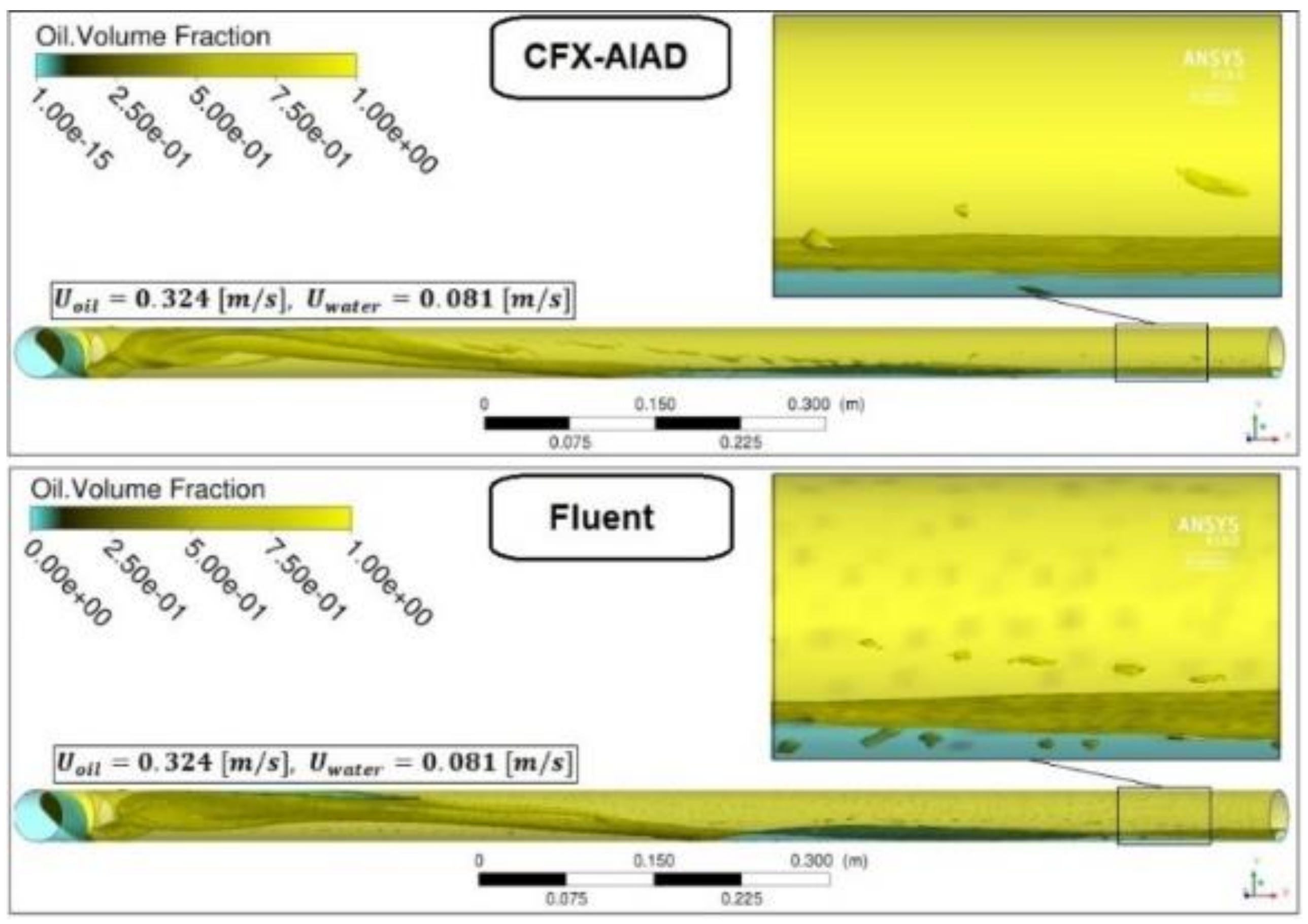
Figure 7 shows the iso-surface of the volume fraction of oil in the entire domain. After the oil and water meet, turbulent structures start developing at the beginning of the mixing T-section. This plays a major role in the flow configuration as it moves through the pipe. For example, at high oil velocity of Uoil = 0.324 m/s and at low water velocity of 0.081 m/s, oil is distributed throughout the pipe. One very noticeable fact from Figure 7 is that the default Multi-Fluid VOF approach seems to be unable to maintain the proper stability and stratification of the interface, breaking the surface into a large range of seemly unphysical droplets. Without the proper modeling capabilities of a regime transition approach such as with AIAD, it does not seem possible to maintain the proper integrity of the interface. This is not the case when using AIAD in CFX as it is shown in the next section.
When looking at the course of the oil and water phases in Figure 8 and Figure 9, it is noticeable that the flow does not follow a clear stratification (multiple peaks in velocity distribution), as it would be expected based on the previous observations from the qualitative data. These are all issues known to occur in free-surfaces approaches without proper treatment of the interface such as the one AIAD offers.
7.2. CFX Results (with AIAD)
Figure 10 shows the oil volume fraction of the four cases. At the water velocity Uwater = 0.081 m/s and the oil velocity Uoil = 0.122 m/s the two phases are separated. As the oil velocity increases to 0.324 m/s, it becomes dominant throughout the pipe.
The unphysical formation of droplets from free-surface destabilization is significantly less pronounced in comparison to the Multi-Fluid VOF approach without AIAD. As the mass flow rate of water increases, the flow of oil and water at the interface becomes turbulent and shows clear interpenetration of both fluids.
Different from the non-AIAD results (Figure 11), the data shown in Figure 8 present a clear and more logical stratification of the flow in the four data sets. Even in the most turbulent cases, the correct treatment of the drag, interfacial area, and subgrid turbulence, help producing more realistic results in comparison to the experimental data.
7.3. Comparison of the Results between CFX-AIAD, Fluent without AIAD and the Experimental Data
For comparison between the calculation results and the experimental results, snapshots of the volume fraction were generated after the flow is developed.
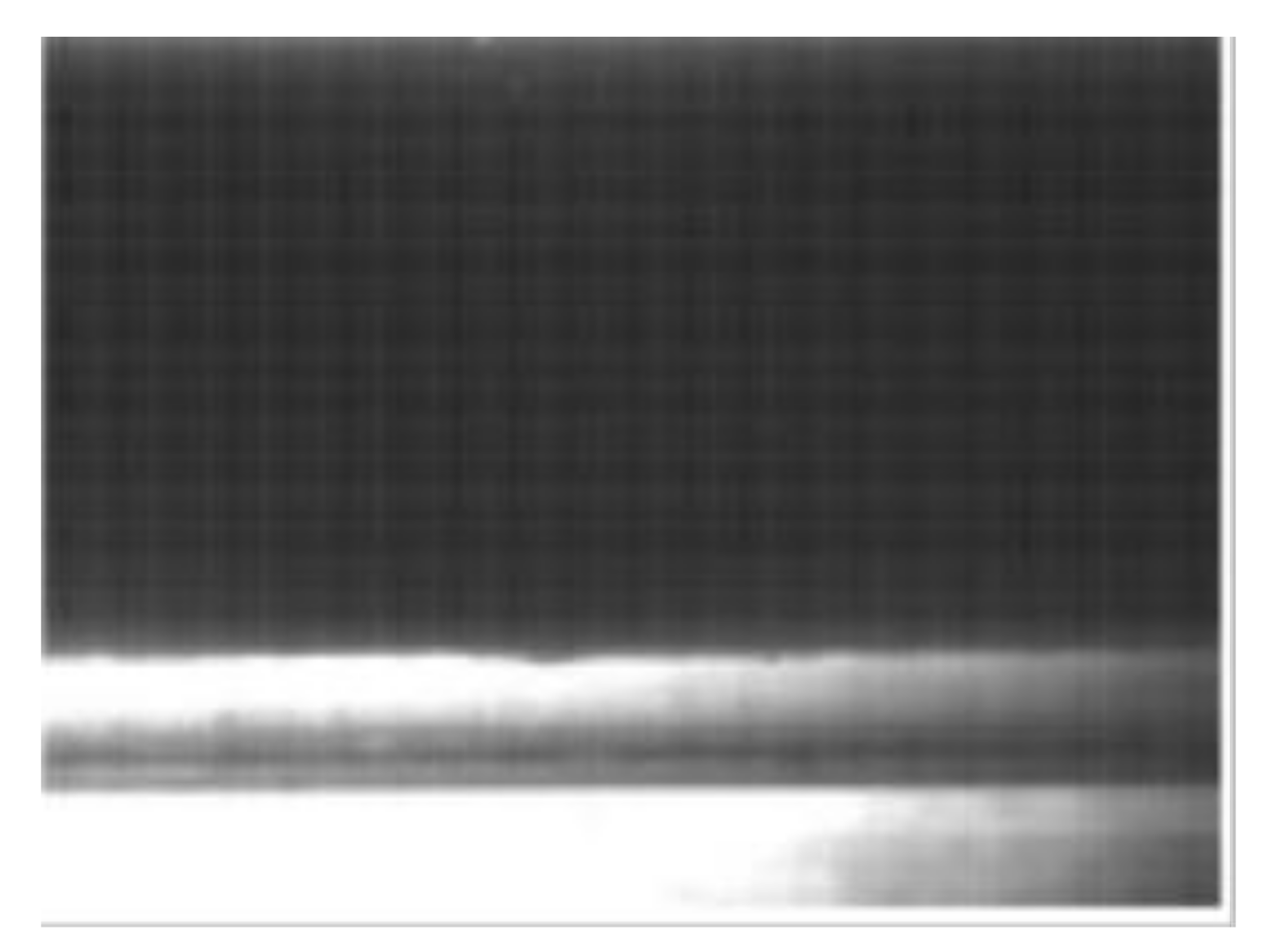
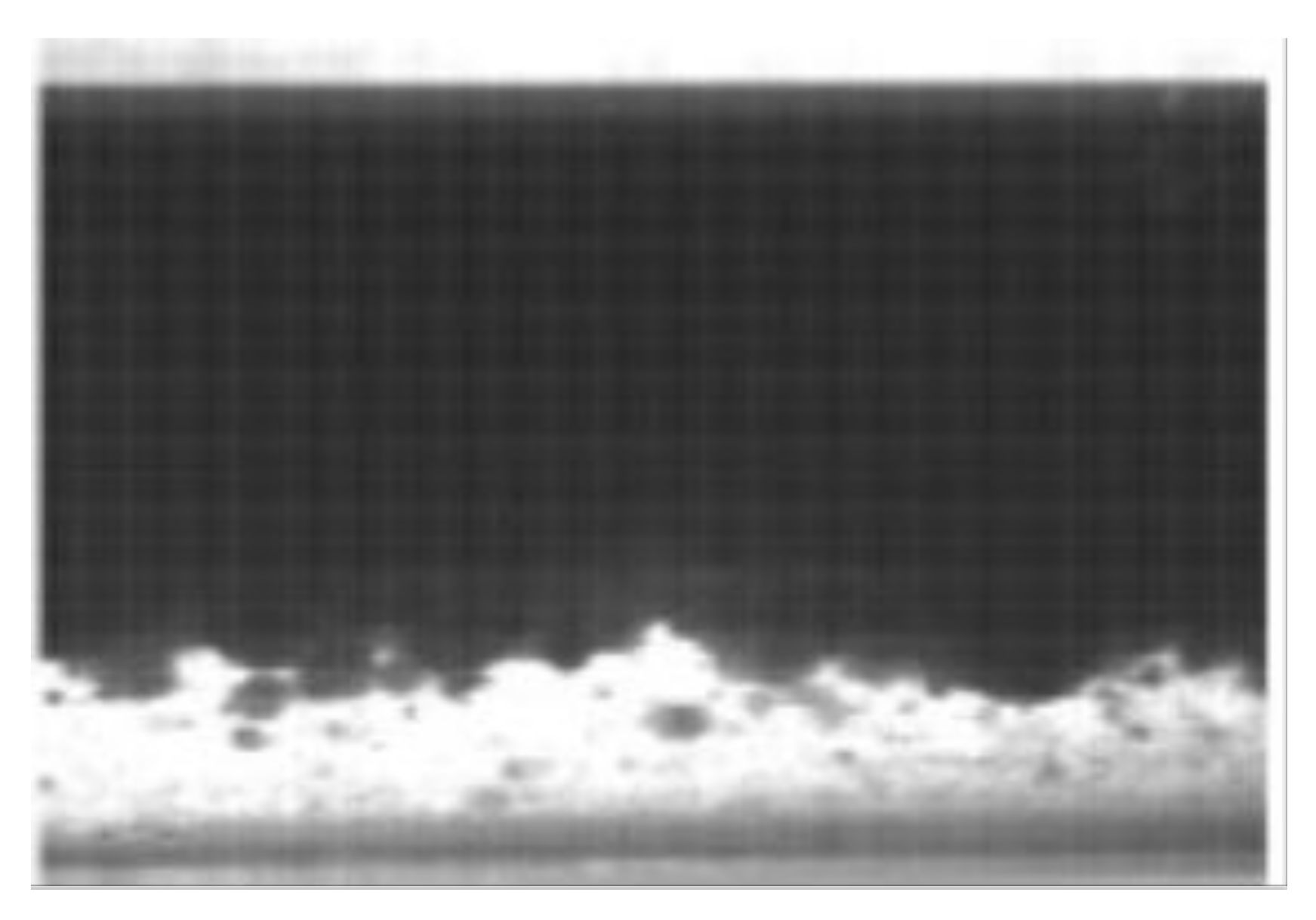
In the first case Uoil = 0.324 m/s and Uwater = 0.081 m/s (Figure 12). In this case, the results without AIAD show unphysical formation of droplets, while the case with AIAD shows qualitative results with a more stable stratification, similar to the experimental data (Figure 13).
Figure 12.
Flow pattern at Uoil = 0.324 m/s, Uwater = 0.081 m/s—experiment [11].

Figure 13.
Oil volume fraction in the entire domain at Uoil = 0.324 m/s and Uwater = 0.081 m/s.
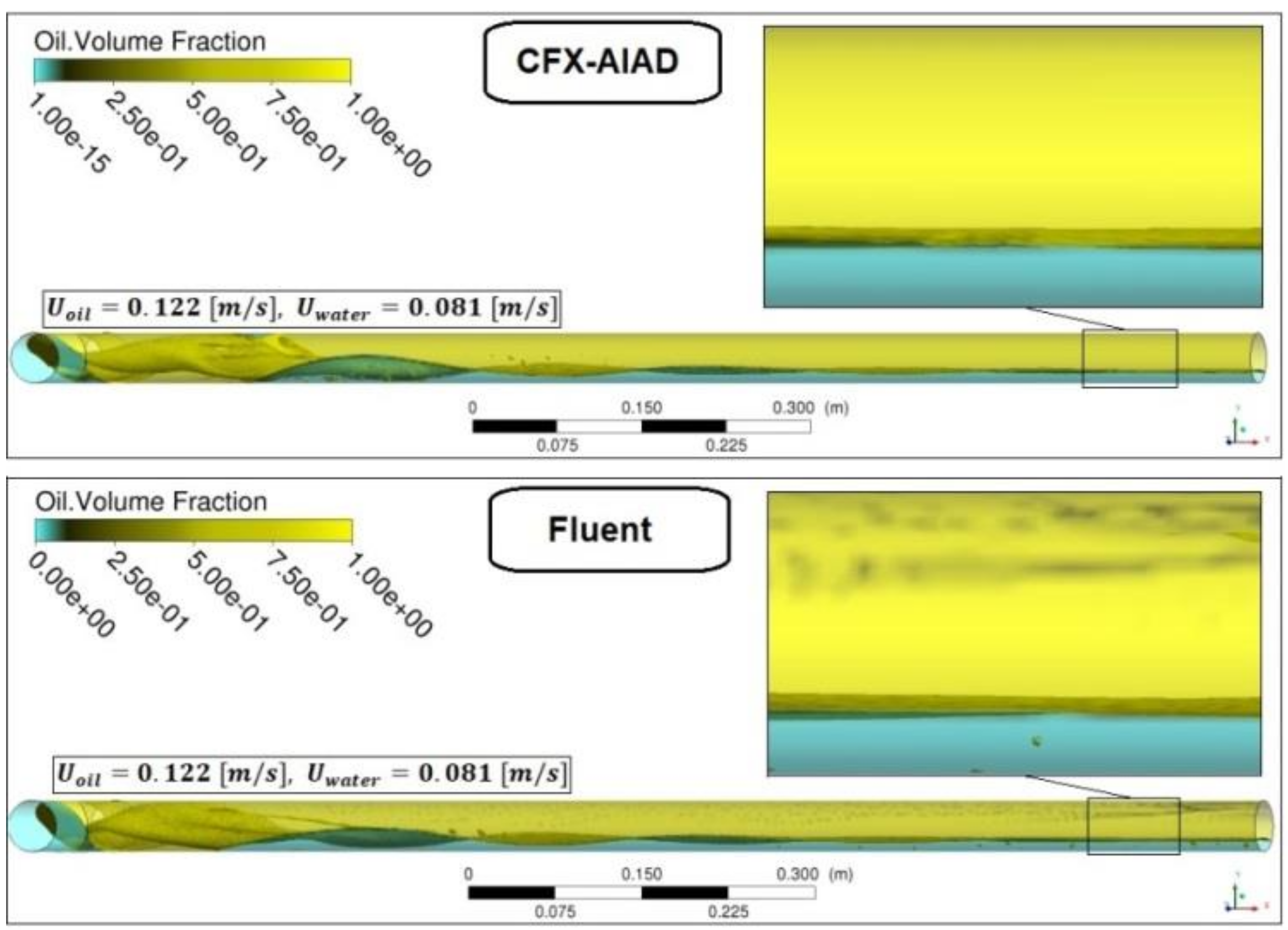
In the second case where Uoil = 0.122 m/s and Uwater = 0.081 m/s, the flow was stratified (ST) similarly to the previous experimental point (Figure 14). While in this case both the calculation with and without AIAD show similar results between them, the case with AIAD showed a better resolution for the oil phase (Figure 15).

Figure 14.
Flow pattern at Uoil = 0.122 m/s, Uwater = 0.081 m/s—experiment [11].
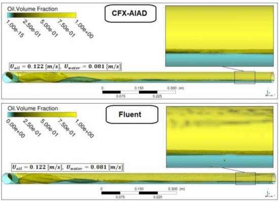
Figure 15.
Oil volume fraction in the entire domain at Uoil = 0.122 m/s, Uwater = 0.081 m/s.
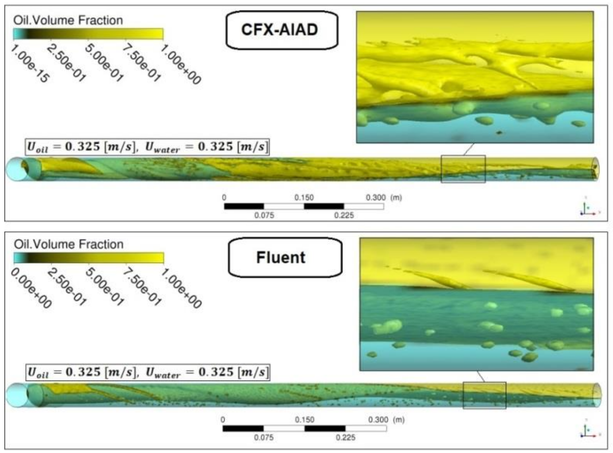
In the third case, the experiment presents oil and water velocities as Uoil = 0.325 m/s and Uwater = 0.325 m/s. Here, the flow is stratified and mixed (ST & MI) with oil droplets incursion into the water phase (Figure 16). The results with AIAD clearly presents a more realistic behavior clearly showing the waves produced at the interface. The small wave turbulence at the interface between the two phases are achieved in AIAD by considering turbulence damping and sub-grid wave turbulence [12]. This behavior cannot be captured in the case without AIAD (Figure 17).

Figure 16.
Flow pattern at Uoil = 0.325 m/s, Uwater = 0.325 m/s—experiment [11].

Figure 17.
Oil volume fraction in the entire domain at Uoil = 0.325 m/s, Uwater = 0.325 m/s.
For the fourth case where Uoil = 0.122 m/s and Uwater = 0.284 m/s, the experiment clearly shows a disperse flow pattern of small oil droplets in the aqueous phase (DO/W & W) (Figure 18). None of the two cases managed to capture the proper entrainment of droplets inside the liquid phase (Figure 19).
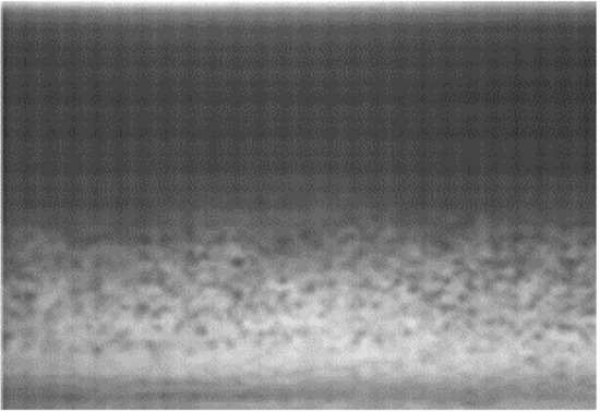
Figure 18.
Flow pattern at Uoil = 0.122 m/s, Uwater = 0.284 m/s—experiment [11].
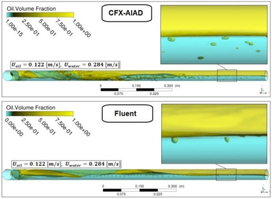
Figure 19.
Oil volume fraction in the entire domain at Uoil = 0.122 m/s, Uwater = 0.284 m/s.
In the future, FLUENT calculations will be run using AIAD with an entrainment mechanism to allow the correct capturing of the entrained droplets as a dispersed Eulerian phase [20].
8. Conclusions and Outlook
Diverse flow patterns for the horizontal pipes were characterized following the classification used by Trallero [6], then the experimental images were processed. With the Euler–Euler Model in FLUENT, where a velocity field for each phase exists, it is possible to simulate the oil–water flow. The interaction or interpenetration of the droplets from one phase to another phase of the oil–water flow can be significantly influenced by the continuum surface force. Also, the AIAD model in ANSYS CFX solver is able to model the oil–water flow. The interfacial forces and the turbulence damping between oil and water play an important role in the interfacial dynamics. Further steps following this publication will be to validate the AIAD model as implemented in FLUENT 2020 R1 software against a larger range of oil–water experiments, including different pipe inclinations. The AIAD implementation in FLUENT takes care of not only the blending of drag and interfacial area, but also of turbulence damping, subgrid turbulence modeling, and entrainment and absorption mechanism into a different dispersed phase. The biggest advantage of that is the possibility of further growth via population balance mechanisms.
Author Contributions
Data curation, G.M.; Funding acquisition, T.H.; Investigation, T.H. and G.M.; Project administration, T.H.; Software, G.M.; Supervision, T.H.; Validation, A.R.; Visualization, A.R.; Writing—original draft, T.H. and A.R.; Writing—review & editing, T.H. and G.M. All authors have read and agreed to the published version of the manuscript.
Funding
This research received no external funding.
Acknowledgments
The authors would like to acknowledge the Thermodynamics and Transport Phenomena Department of the University Simon Bolivar (USB) for allowing the use of the hereby presented protected data via their agreement with Dr. Gustavo Montoya.
Conflicts of Interest
The authors declare no conflict of interest.
References
- Höhne, T.; Porombka, P. Modelling horizontal two-phase flows using generalized models. Ann. Nuclear Energy 2018, 111, 311–316. [Google Scholar]
- Walvekar, R.G.; Choong, T.S.; Hussain, S.; Khalid, M.; Chuah, T. Numerical study of dispersed oil–water turbulent flow in horizontal tube. J. Pet. Sci. Eng. 2009, 65, 123–128. [Google Scholar] [CrossRef]
- Burlutskii, E. CFD study of oil-in-water two-phase flow in horizontal and vertical pipes. J. Pet. Sci. Eng. 2018, 162, 524–531. [Google Scholar] [CrossRef]
- Shi, J.; Gourma, M.; Yeung, H. CFD simulation of horizontal oil-water flow with matched density and medium viscosity ratio in different flow regimes. J. Pet. Sci. Eng. 2017, 151, 373–383. [Google Scholar]
- Hessel, V.; Angeli, P.; Gavriilidis, A.; Lowe, H. Gas–liquid and gas–liquid–solid microstructure reactors: Contacting principles and applications. Ind. Eng. Chem. Res. 2005, 44, 9750–9769. [Google Scholar] [CrossRef]
- Trallero, J.L.; Shariah, C.; Brill, J.P. A Study of Oil-Water Flow Patterns in Horizontal Pipes. In Proceedings of the Annual Technical Conference and Exhibition, Denver, CO, USA, 6–9 October 1996; Volume 1, pp. 363–375. [Google Scholar]
- Torres, C.F.; Mohan, R.S.; Gomez, L.E.; Shoham, O. Oil-Water Flow Pattern Transition Prediction in Horizontal Pipes. J. Energy Resour. Technol. 2016, 138, 022904. [Google Scholar]
- Montoya, G.; Valecillos, M.; Romero, C.; Gonzales, D. Determination of Hydrodynamic Parameters on Two-Phase Flow Gas-Liquid in Pipes with Different Inclination Angles Using Image Processing Algorithm. In Proceedings of the 62 Annual Meeting of the American Physical Society’s Division of Fluid Dynamics (DFD), Minneapolis, MI, USA, 22–24 November 2009. [Google Scholar]
- Montoya, G.; Garcia, K.; Valecillos, M.; Garcia, J.; Romero, C.; González, D. Determinación de altura de fase y hold up para flujo bifásico liquido-liquido en tuberías horizontales por medio de procesamiento de imágenes. In Proceedings of the American Society of Mechanical Engineers (ASME) Congress “Ideas Practicas Soluciones Eficientes”, University Simon Bolivar (USB), Caracas, Venezuela, 26–28 November 2009. [Google Scholar]
- Montoya, G.; Valecillos, M.; Romero, C.; González, D. Determination of hydrodynamic parameters on two-phase flow gas-liquid in pipes with different inclination’s angles using image processing algorithm. In Proceedings of the International Conference on Multiphase Flow (ICMF-2010), Tampa, FL, USA, 30 May–4 June 2010. [Google Scholar]
- Montoya, G.; Valecillos, M.; Garcia, J.; Romero, C.; González, D. Determination and study of hold up and flow patterns in two-phase flow liquid-liquid systems for horizontal and inclined pipes using image processing techniques. In Proceedings of the International Conference on Multiphase Flow (ICMF-2010), Tampa, FL, USA, 30 May–4 June 2010. [Google Scholar]
- Höhne, T.; Porombka, P.; Moya Sáez, S. Validation of AIAD Sub-Models for Advanced Numerical Modelling of Horizontal Two-Phase Flows. Fluids 2020, 5, 102. [Google Scholar] [CrossRef]
- Höhne, T.; Mehlhoop, J.P. Validation of closure models for interfacial drag and turbulence in numerical simulations of horizontal stratified gas-liquid flows. Int. J. Multiph. Flow 2014, 62, 1–16. [Google Scholar] [CrossRef]
- Griffith, P.; Wallis, G.B. Two-phase slug flow. J. Heat Transf. 1961, 83, 307. [Google Scholar]
- Taitel, Y.; Bornea, D.; Dukler, A.E. Modelling Flow Pattern Transitions for Steady Upward Gas-Liquid Flow in Vertical Tubes. AlChE J. 1980, 26, 345–354. [Google Scholar] [CrossRef]
- Murzyn, F.; Chanson, H. Experimental investigation of bubbly flow and turbulence in hydraulic jumps. Environ. Fluid Mech. 2009, 9, 143–159. [Google Scholar] [CrossRef]
- Wilcox, D.C. Turbulence Modelling for CFD; DCW Industries Inc.: La Cañada, CA, USA, 1994. [Google Scholar]
- Brocchini, M.; Peregrine, D.H. The dynamics of strong turbulence at free surfaces. Part1. Description. J. Fluid Mech. 2001, 449, 225–254. [Google Scholar] [CrossRef]
- Mahaffy, J.; Chung, B.; Song, C.; Dubois, F.; Graffard, E.; Ducros, F.; Heitsch, M.; Scheuerer, M.; Henriksson, M.; Komen, E.; et al. Best Practice Guidelines for the Use of CFD in Nuclear Reactor Safety Applications-Revision; NEA/CSNI/R(2014)11; Organisation for Economic Co-Operation and Development: Paris, France, 2015. [Google Scholar]
- Höhne, T.; Hänsch, S. A droplet entrainment model for horizontal segregated flows. Nuclear Eng. Des. 2015, 286, 18–26. [Google Scholar]


© 2020 by the authors. Licensee MDPI, Basel, Switzerland. This article is an open access article distributed under the terms and conditions of the Creative Commons Attribution (CC BY) license (http://creativecommons.org/licenses/by/4.0/).