Coastal Wind Power in Southern Santa Catarina, Brazil

Abstract

A light detection and ranging (LIDAR) wind profiler was used to estimate the wind speed in the southern coast of Santa Catarina State, Brazil. This profiler was installed on a coastal platform 250 m from the beach, and recorded wind speed and direction from January 2017 to December 2018. The power generation from three wind turbines was simulated, to obtain estimations of the average power, energy generation and capacity factor, as well as to assess the performance of a hypothetical wind farm. The scale and shape parameters of the Weibull distribution were evaluated and compared with those of other localities in the state. The prevailing winds tend to blow predominantly from the northeast and southwest directions. Wind magnitudes are higher for the NE and SW ocean sectors where the average wind power density can reach 610–820 W m⁻². The Vestas 3.0 turbine spent the largest percentage of time in operation (>76%). The higher incidence of strong northeasterly winds in 2017 and more frequent passage of cold fronts in 2018 were attributed to the cycle of the South Atlantic subtropical high. The results demonstrate a significant coastal wind power potential, and suggest that there is a significant increase of resources offshore.

1. Introduction

Wind energy is one of the most promising renewable alternatives available for exploitation in Brazil today [1]. It is a mature technology, and the resource is significant and cost-competitive compared with other energy sources. Until now, all wind farms have been situated in continental areas, where they account for 15.52 GW or 9% of the national installed capacity [2]. It is expected that wind power will reach 19 GW by 2024, an increase of 22.7% in installed wind capacity [3].

There are still vast areas available for continental exploitation in Brazil, although conflicts over land use have been reported [4,5]. The exploitation of offshore wind energy appears to be an alternative to wind energy development [6]. Although offshore turbines incur larger installation and operational costs, the force of winds is of a stronger magnitude over the ocean [7,8,9]. Offshore wind farms generally operate at larger capacity factors and the investment in these projects tends to have similar return periods to those of onshore wind farms.

The power of Brazil’s offshore wind is estimated to be between 1300 GW and 1800 GW for installations up to 100 m in depth [10,11]. However, there is a very limited meteorological buoy network and the country lacks a program for long-term monitoring of coastal winds at the height of wind turbines. Despite this, the quality of its winds has aroused considerable interest in the energy sector. In 2018, Petrobras announced that the first Brazilian offshore wind turbine would be installed in Guamaré, Rio Grande do Norte [12]. Until January 2020, Brazil had six projects for offshore wind farms with applications for environmental licensing underway at the Brazilian Institute of the Environment and Renewable Natural Resources (IBAMA) for the States of Rio Grande do Sul, Rio de Janeiro, Rio Grande do Norte, and Ceará [11]. There are notable resources that lie in the north, northeast, southeast, and southern regions of Brazil [10,11,13].

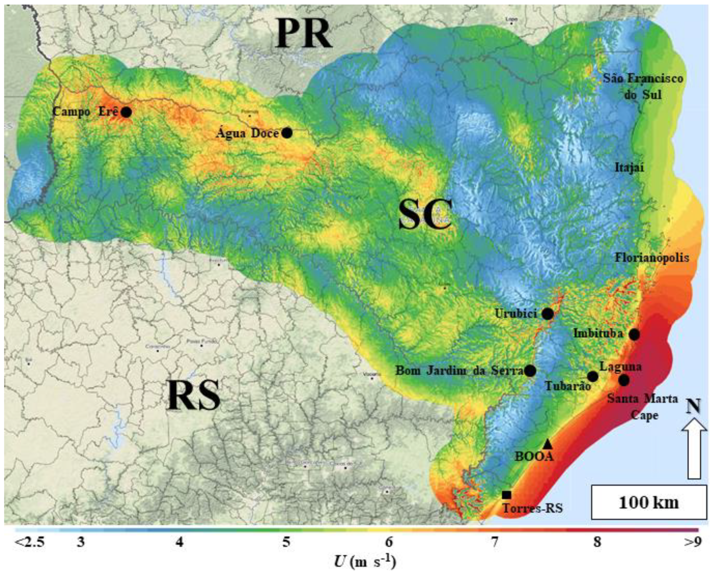
The State of Santa Catarina has promising regions for development in continental and offshore areas, as illustrated by the wind speed fields derived from the Global Wind Atlas [14] which shows the average wind climatology for the height of 100 m above the terrain/sea surface (Figure 1). Here the red colors indicate high wind speeds, exceeding 8 m s⁻¹. Shades in blue indicate weaker winds, below 4 m s⁻¹.

As shown, there are continental wind resources present in the western highlands of the state, the central region, the coastal mountains, and the coastal plain near Laguna and Santa Marta Cape.

The state contribution to the national generation of energy is 4803.7 MW, where 3415.2 MW comes from hydropower [2]. The wind-installed capacity is only 245.5 MW with all its farms being located in continental areas: Água Doce (146.8 MW), Bom Jardim da Serra (93.6 MW), Laguna (3.0 MW), and Tubarão (2.1 MW) [16] (see wind farm locations in Figure 1).

Offshore wind resources are significant. The map illustrates large changes of ocean wind speeds in different latitudes. Average winds vary from 5 m s⁻¹ in the north of the state off São Francisco do Sul to more than 9 m s⁻¹ offshore of Cape Santa Marta (Figure 1). The estimated offshore potential in a depth of between 0 and 500 m is around 184 GW, based on the analysis of outputs from the statistical downscaling model [17].

There is a serious lack of wind observational studies for Santa Catarina. In the continental region, Dalmaz (2007) conducted an analysis of winds from six anemometric towers of 48 m, installed in Água Doce, Bom Jardim da Serra, Campo Erê, Imbituba, Laguna, and Urubici (see sites of towers in Figure 1) [15]. Here we analyze a new dataset obtained with a Light Detection and Ranging (LIDAR) wind profiler installed in the Ocean and Atmosphere Observation Base (BOOA) coastal laboratory (Figure 1). BOOA was built over a fishing platform about 250 m from the beach of Balneário Arroio do Silva, in Southern Santa Catarina. The laboratory provides electrical power and support for the LIDAR and has a meteorological tower (Figure 2).

A preliminary analysis of the first 6 months of LIDAR wind data was conducted by Correa (2018) [17], Nassif et al. (2020) [18] and Pires (2019) [19]. Here we extend the period of analysis, and cover two years of data from January 2017 to December 2018. This study describes the average power, mean capacity factor and energy generated by modern wind turbines at BOOA. It also makes a comparison of the LIDAR data with the statistical parameters derived from the towers, as reported by Dalmaz (2007).

Thus, the aim of this study is to describe the estimated wind power from a coastal site in Southern Brazil using LIDAR profiler measurements between 2017 and 2018. It takes account of the synoptic behavior, its monthly and interannual variability, estimations for a hypothetical wind farm, and comparisons with wind resources from other locations of Santa Catarina State.

Although other studies have employed LIDAR in the world’s coastal and offshore regions to assess wind resources [20,21,22,23,24,25,26,27,28], few studies have investigated LIDAR observations in Brazil. Two pioneer studies monitored winds on the coast of Piauí [29,30], one for Espírito Santo State [31]. Thus, this dataset represents the longest period of LIDAR wind monitoring conducted for the southern coast of the country. The present paper comes at an opportune moment to foster and support the current process of offshore wind energy planning, and underlines the importance of long-term wind profile monitoring for the Brazilian coast.

2. Data and Methods

In this section, we provide an outline of the data and methods used in this study. The first part describes the key features of LIDAR and the observation base built over the fishing platform. Following this, we describe the various parameters estimated from LIDAR data, such as the power density, turbine power, generated energy, capacity factor, and Weibull distribution.

2.1. LIDAR Profiler

The LIDAR profiler was installed on the Entremares Fishing Platform, located at Balneário Arroio do Silva in the southern coast of Santa Catarina (Figure 2). The platform consists of a 7 m wide concrete structure that advances into the ocean, with a total length of 410 m (Figure 2a). A laboratory called Ocean and Atmosphere Observation Base (BOOA) with 2 × 2 m internal dimensions and a height of 2.5 m was built near the end of the platform to provide power and support for the LIDAR (Figure 2b). The shoreline is at an angle of approximately 45° from the geographic north. A meteorological tower was installed on the top of BOOA. The met station was equipped with a Dualbase SDITH-01 thermo-hygrometer with a cover to protect it from sunlight, and installed at a height of 11 m above the mean sea level. A Young Sonic 81,000 3D anemometer was installed at 19.7 m above the ocean surface (Figure 2b). An atmospheric pressure sensor was also installed inside the laboratory.

The model of the LIDAR profiler is Z300 Offshore manufactured by ZephIR. The devices continuously emit an infrared laser, as a means of measuring the speed and direction of winds between 10 and 300 m above the equipment at 11 different levels [32]. The LIDAR is located 9.6 m above mean sea level. In this study, winds at the height of 20, 49, and 110 m above mean sea level were selected for analysis.

The devices provide data at 10-min average intervals calculated from the raw data. The dataset covers 94.09% of the period between January 2017 and December 2018 for the height of 110 m and 94.34% for the height of 49 m. The reason for the short periods without data collection was that the LIDAR was used in other field campaigns conducted in September 19 to 22, 2017 (four days) and November 5 to 26, 2017 (22 days). In 2018, there were other significant gaps from October 27 to 29 (ca. three days), November 17 to 20 (ca. three days), and December 13 and 18 (ca. six days).

2.2. Power Density

The wind power resource assessment used theoretical processes for estimating the power density equation, which provides the flow of kinetic energy contained in the wind [33]. This equation is expressed as:

$$D_p=\frac{1}{2}{\rho }_a{U}^3,$$

(1)

where D_p (W m⁻²) is the power density, ρ_a is the local air density (kg m⁻³), and U is the horizontal wind speed at a height of 110 m.

Air density ρ_a was calculated with air temperature T (°C), relative humidity RH (%), and atmospheric pressure P (hPa) records from BOOA, following [18]. The data gaps were covered by information from the Torres meteorological station, supplied by the National Institute of Meteorology (INMET) (Figure 1). BOOA T, RH, and P time series covered nearly 98.52% of the period, while 1.48% was supplied by the Torres met station.

2.3. Wind Power Output

Wind turbines are not able to extract all the kinetic energy contained in wind and in practice speed-power curves are used to calculate the power generated by each turbine [34]. Three large-bladed horizontal axis turbines suitable for marine use, were adopted in this study (Vestas 8.0 MW, Senvion 6.2 MW, and Vestas 3.0 MW). The key features of each turbine are described in

Table 1. Features of the three wind turbines selected for wind speed simulations.

	Vestas V112 3.0	Senvion 152 6.2	Vestas V164 8.0
Rated power PT (MW)	3	6.15	8
Cut-in speed UP (m s−1)	3	3.5	4
Cut-out speed UD (m s−1)	25	30	25
Rated speed UR (m s−1)	12.4	11.5	13
Rotor diameter (m)	90	152	164
Swept area (m2)	6362	18,146	21,124

.

Empirical velocity-power curves, P_T = f(U) (MW) are supplied by manufacturers (not shown) and used for power estimation. This cut-in speed of wind turbines ranges from 3.5 to 4.0 m s⁻¹, with rated speeds between 11.5 and 15 m s⁻¹ (Table 1).

2.4. Generated Energy

The energy generated in a given period of time can be defined by the time-integral of the power generated by the turbine [33]. Numerically, this integral can be simplified by:

$$E_g=\frac{{\displaystyle \sum _{i=1}^N{P}_T\left(U_i\right)}\left(\Delta t\right)}{1000},$$

(2)

where N refers to the number of observations, P_T is the turbine output in MW, U_i represents observations of the wind speed at a height of 110 m, Δt is the time interval in hours, and E_g is the generated energy in GWh.

2.5. Capacity Factor

The ratio between the average power generated by a turbine $\overline{P_T}$ and the rated power of the turbine P_R defines the capacity factor CF [33]:

$$CF=\frac{\frac{1}{N}{\displaystyle \sum _{i=1}^N{P}_T\left(U_i\right)}}{P_R}=\frac{\overline{P_T}}{P_R}.$$

(3)

2.6. Probability Distributions

A compact form of wind regime characterization can be achieved by analyzing the wind speed probability distribution functions (PDFs). The two-parameter Weibull distribution curve is given by the following equation [33,35]:

$$PDF\left(U\right)=\left(\frac{k}{c}\right){\left(\frac{U}{c}\right)}^{k-1}\exp \left[{\left(\frac{U}{c}\right)}^k\right],$$

(4)

where k and c represent the shape and scale parameters, respectively.

By integrating the PDF, we can find the cumulative distribution function (CDF):

$$CDF\left(U\right)=1-\exp \left[{\left(\frac{U}{c}\right)}^k\right].$$

(5)

The CDF shows the percentage of time the wind speed is below a certain value and it can be combined with the turbine’s velocity-power curves to obtain the cumulative distribution function of power. The Maximum Likelihood Method (MLM) [36,37] was employed to estimate the k and c Weibull parameters for all the BOOA observations. The MLM has proven to achieve a very good performance compared with other methods employed for the two-parameter estimation [38,39,40].

3. Results and Discussion

LIDAR measurements at the BOOA covered a period of approximately two years, from January 2017 to December 2018. Our analyses first address wind speed and direction, wind power density, turbine power, and generated energy for each year. The probability curves are shown and, in sequence, the interannual variability is explained from the perspective of the South Atlantic Atmospheric Circulation. Finally, a detailed analysis of the monthly variability is conducted, along with a comparison with other localities in the State.

3.1. Wind Variability in 2017–2018

3.1.1. Wind Speed and Direction

Figure 3 illustrates the LIDAR wind speed U and direction θ, the corresponding power density D_p, turbine output P_T, and generated energy E_g for 2017 and 2018. All the variables refer to a height of 110 m.

The wind speed graphs for 2017 and 2018 are displayed in Figure 3a with 10 min time resolution. In these panels, the upper yellow solid line represents the mean rated speed U_R for the selected turbines (12.3 m s⁻¹), and the lower line represents the mean cut-in speed U_P (3.5 m s⁻¹). In 2017, $\overline{U}$ = 6.3 m s⁻¹ and σ = 3.8 m s⁻¹ and, in 2018, $\overline{U}$ = 5.8 m s⁻¹ and σ = 3.6 m s⁻¹, resulting in $\overline{U}$ 8.3% lower than 2017. As illustrated, around 70% of the time, the wind speed was within the turbine’s operational range, and several times exceeded the rated speed (~7%). These periods of activity will be examined in further detail in Section 3.2.

The wind direction time series θ is shown in Figure 3b. Here the daily averages of the wind direction are included for a better visualization. The blue line represents the northeast direction (NE) and the green line the southwest direction (SW). The light blue and light green shades represent the ocean and continental sectors, respectively. There are two predominant wind patterns in the region [41]. The main pattern is from the NE quadrant (30°–60°), which is found approximately 23.5% of the time with the mean wind direction $\overline{\theta }$ = 45.2° and speed $\overline{U}$ = 8.4 m s⁻¹ in 2017. In the case of 2018, winds from the NE quadrant were less frequent and intense, blowing 12.9% of the time with $\overline{\theta }$ = 45.9° and $\overline{U}$ = 6.9 m s⁻¹ (Figure 3b). These winds are a manifestation of the average circulation induced by the South Atlantic subtropical high-pressure system (SASH) [42] and the reasons for the variability between these years will be explored in Section 3.3.

The second predominant directional sector is linked to southwesterly winds (−150° to −120°), mostly cold front passages. The winds came from the SW quadrant during 11.1% of the time and resulted in $\overline{\theta }$ = −135.4° and $\overline{U}$ = 7.1 m s⁻¹ during 2017. In 2018, $\overline{\theta }$ = −135.2° and $\overline{U}$ = 7.1 m s⁻¹ with a time fraction of 16.5%. Cold fronts accompany the displacement of mobile cyclones and anticyclones in the southern region of Brazil [43] and originate from three cyclogenetic regions in the western sector of the South Atlantic Ocean, near the South American east coast [44]. In this studied region, there is usually a passage of up to four cold fronts per month with an increase in the spring [45]. During the passages, the winds tend to intensify and change their direction [46]. This intensification leads to an increase in turbine production.

The winds were less intense in the NE quadrant and had a larger influence on the SW continental sector in 2018 (Figure 3b). There was a 10.6% decrease in the frequency of northeasterly winds from 2017 to 2018, while southwesterly winds increased by approximately 5.4%. The bimodal directional distribution and its interannual wind variability are well represented in the directional wind speed histograms (Figure 4a,b).

Directional statistical parameters were estimated for each year from the LIDAR data at 110 m height (

Table 2. Statistical distribution of wind parameters. BOOA represent winds from all directions. BOOA NE sector and BOOA SW sector represent the winds from 45° ± 90° and −135° ± 90° directions, respectively. N is the number of observations. $\overline{\theta }$ is the average wind direction. d represents the range for 95% confidence limits. R is the mean resultant vector length.

	BOOA		BOOA (NE-Sector)		BOOA (SW-Sector)
	2017	2018	2017	2018	2017	2018
N	48,572	50,337	28,553	23,260	200,019	27,077
$\overline{\theta }$ ± d (°)	40.15 ± 2.15	172.25 ± 3.70	43.40 ± 0.48	51.63 ± 0.58	−134.82 ± 0.65	−140.00 ± 0.54
R	0.17	0.10	0.80	0.76	0.74	0.76

). The parameters were calculated by taking account of all the wind directions in BOOA, and also specific sectors denoted as ${\theta }_0\pm \delta \theta$ where δθ is 90° and ${\theta }_0$ = 45° for the NE sector and ${\theta }_0$ = −135° for the SW sector. The mean wind direction $\overline{\theta }$, their confidence limits (range d) and the resultant vector length (R) were estimated by following Berens (2009) [47] (Table 2). Here, R represents a measure of the circular spreading, which is related to variance by S = (1 − R). If all samples point in the same direction, R is close to 1 and S is small. Correspondingly, if the samples are spread out evenly in all directions, R is small and S is close to 1. $\overline{\theta }$ is not defined for R = 0 [47,48].

The mean direction was $\overline{\theta }$ = 40.15° in 2017, with a 95% confidence interval range of d = ±2.15°. In 2018, $\overline{\theta }$ = 172.25° with d = ±3.70°. These results corroborate the degree of interannual variability, with a greater dominance of NE winds in 2017 and more influence of SW winds in 2018. R is low for both years, but relatively larger for 2017, which is evidence of the dominance of the NE winds.

When the same parameters were applied to the NE sector, it showed that, in 2017, the winds blew in a direction more parallel to the coastline, with mean direction $\overline{\theta }$ = 43.40° ± 0.48°, while in 2018, the winds were slightly displaced offshore with $\overline{\theta }$ = 51.63° ± 0.58°. Winds from the SW sector showed $\overline{\theta }$ = −134.82° ± 0.65° in 2017 and a more offshore component with $\overline{\theta }$ = −140.00° ± 0.54° in 2018. The resultant vector length R for the NE- and SW sectors was above 0.74 in both years, which suggests there was a reduced directional spread. The largest R = 0.8 was observed in 2017 for the NE sector (Table 2).

Owing to the bimodal nature of wind directions at BOOA, the circular-linear correlation ρ_cl between wind direction and speed was evaluated separately for both sectors, resulting in mild correlations ρ_cl = 0.40 for the NE sector and ρ_cl = 0.35 for the SW sector. Finally, the LIDAR direction at 20 m correlated with the Sonic anemometer direction at 19.7 m, which yielded a very good circular-circular correlation ρ_cc = 0.81 for BOOA using 21,557 10 min paired means of wind direction [19,47].

3.1.2. Wind Power Density

The 10 min mean time series of D_p is illustrated in Figure 3c. In 2017 and 2018, the mean power density $\overline{D_p}$ was 333.4 W m⁻² and 272.2 W m⁻², respectively. In 2017, the maximum D_p (7760.4 W m⁻²) occurred on December 17 at 6:40 p.m. However, in 2018, the maximum D_p (8509.1 W m⁻²) occurred on September 23 at 9:30 a.m. In both years, the D_p peaks are higher and more frequent in the second semester, with some peaks exceeding 6000 W m⁻².

The directional mean distribution of D_p is examined in further detail in Figure 4c,d, through the calculation of average power density for 10° directional sectors. As seen earlier, winds from ocean sectors (NE and SW) have higher D_p for both years. In the NE sector, the peak was $\overline{D_p}$ = 826.4 W m⁻² between 50° and 60° in 2017. In 2018, the peak was $\overline{D_p}$ = 681.6 W m⁻² between 60° and 70°. In the case of the SW sector, the peak was $\overline{D_p}$ = 615.3 W m⁻² between −160° and −150° in 2017. In 2018, the peak was $\overline{D_p}$ = 546.7 W m⁻² between −130° and −120°. The average power density of these sectors tends to be much greater than for other directions. This demonstrates that the bulk of the power is found in winds that blow nearly parallel to the coastline, but predominantly from the ocean sectors (NE and SW). Winds perpendicular to the coast have very low energy content. Figure 4 shows the importance of ocean winds to coastal wind power generation. The estimated power density from satellite data and numerical modeling, suggest that offshore resources vary seasonally from 600 to 900 W m⁻² [13,14,17].

3.1.3. Turbine Output

The time series for turbine output is illustrated in Figure 3d for the Vestas 3.0 (blue), Senvion 6.2 (red), and Vestas 8.0 (gray) turbines. The key features of the turbines are described in Table 1. In 2017, turbine mean output $\overline{P_T}$ (CF) was 2.2 MW for Vestas 8.0 turbine (CF = 27.5%). In the case of Senvion 6.2, this output was 1.8 MW (CF = 29.2%), while for Vestas 3.0, 0.9 MW (CF = 31.5%) (

Table 3. Wind resource, Weibull distribution parameters, and production of the three turbines in monthly and annual averages for the year 2017 from 10 min LIDAR data at 110 m high. Percentage % refers to LIDAR data coverage for the period. $\overline{U}$ is the mean wind speed (m s⁻¹). NE% and SW% are the percentages of northeasterly (45° ± 15°) and southwesterly (−135° ± 15°) winds, respectively. The Weibull scale parameter c (m s⁻¹) and Weibull shape parameter k are indicated. $\overline{D_p}$ is the mean power density (W m⁻²), $\overline{P_T}$ is the mean output per turbine (MW), E_g is the generated energy (GWh), and CF is the capacity factor (%).

	%	$\overline{\mathit{U}}$	NE%	SW%	c	k	$\overline{{\mathit{D}}_{\mathit{p}}}$	Vestas 3.0			Senvion 6.2			Vestas 8.0
								$\overline{{\mathit{P}}_{\mathit{T}}}$	Eg	CF	$\overline{{\mathit{P}}_{\mathit{T}}}$	Eg	CF	$\overline{{\mathit{P}}_{\mathit{T}}}$	Eg	CF
JAN	100	5.4	15.7	6.2	6.08	1.91	185.4	0.7	0.49	22.2	1.2	0.90	19.7	1.5	1.10	18.6
FEB	100	5.8	34.3	4.7	6.56	1.77	254.5	0.8	0.56	28.0	1.6	1.07	25.9	1.9	1.31	24.3
MAR	100	5.7	16.9	7.5	6.48	1.88	232.4	0.8	0.58	25.9	1.4	1.07	23.5	1.8	1.31	22.1
APR	100	5.9	24.5	9.0	6.61	1.81	258.2	0.8	0.61	28.3	1.6	1.15	26.1	1.9	1.40	24.3
MAY	100	6.2	24.8	13.6	6.99	1.68	339.8	0.9	0.69	31.0	1.8	1.32	28.9	2.2	1.62	27.3
JUN	98.9	5.3	16.8	12.7	6.03	1.85	197.5	0.7	0.48	22.6	1.3	0.89	20.4	1.5	1.08	19.1
JUL	98.9	5.6	31.3	6.1	6.34	1.71	250.4	0.8	0.59	26.5	1.5	1.11	24.4	1.8	1.35	22.9
AUG	100	8.1	35.7	12.5	9.13	1.83	668.7	1.4	1.02	45.8	2.7	2.00	43.6	3.3	2.48	41.6
SEP	83.3	7.0	30.4	20.6	7.93	1.91	419.3	1.1	0.69	38.2	2.2	1.32	35.8	2.7	1.61	33.4
OCT	100	7.1	16.9	15.3	7.99	1.72	475.6	1.2	0.89	39.9	2.3	1.73	38.0	2.9	2.14	36.1
NOV	26.7	6.8	12.8	9.7	7.67	1.83	404.2	1.1	0.20	35.7	2.1	0.39	33.5	2.5	0.48	31.6
DEC	100	6.7	16.4	15.1	7.58	1.83	367.6	1.1	0.82	36.8	2.1	1.58	34.5	2.6	1.92	32.4
2017	92.4	6.3	23.5	11.1	7.07	1.75	333.4	0.9	7.64	31.5	1.8	14.56	29.2	2.2	17.84	27.5

). The percentage of time without power generation was 32.8% for Vestas 8.0, 26.8% for Senvion 6.2, and 20.6% for Vestas 3.0. The rated output (maximum turbine capacity) was reached 6.2% of the time for Vestas 8.0, 10.7% for Senvion 6.2, and 7.7% for Vestas 3.0.

In 2018, the $\overline{P_T}$ was 1.9 MW (CF = 23.3%) for Vestas 8.0 turbine. This production was 1.5 MW (CF = 24.8%) for Senvion 6.2 and 3.0, 0.8 MW for Vestas (CF = 26.9%) (

Table 4. Similar to Table 3, but referring to the year 2018.

	%	$\overline{\mathit{U}}$	NE%	SW%	c	k	$\overline{{\mathit{D}}_{\mathit{p}}}$	Vestas 3.0			Senvion 6.2			Vestas 8.0
								$\overline{{\mathit{P}}_{\mathit{T}}}$	Eg	CF	$\overline{{\mathit{P}}_{\mathit{T}}}$	Eg	CF	$\overline{{\mathit{P}}_{\mathit{T}}}$	Eg	CF
JAN	100	5.7	12.4	16.1	6.40	1.76	246.5	0.8	0.57	25.6	1.4	1.07	23.3	1.8	1.31	22.0
FEB	100	5.2	11.3	13.4	5.86	1.83	177.2	0.6	0.43	21.4	1.2	0.79	19.1	1.4	0.96	17.8
MAR	100	5.3	10.7	15.1	6.01	1.70	213.0	0.7	0.52	23.4	1.3	0.97	21.2	1.6	1.19	20.1
APR	100	4.8	10.5	15.0	5.41	1.78	148.1	0.5	0.38	17.8	1.0	0.69	15.7	1.2	0.85	14.7
MAY	99.6	5.1	12.0	15.9	5.77	1.95	158.8	0.6	0.45	20.1	1.1	0.81	17.7	1.3	0.98	16.5
JUN	96.6	5.0	9.4	16.8	5.63	1.69	182.1	0.6	0.43	20.4	1.1	0.79	18.4	1.4	0.96	17.2
JUL	97.3	5.3	9.9	18.6	5.90	1.61	240.3	0.7	0.48	22.1	1.2	0.89	20.1	1.5	1.10	19.1
AUG	95.7	5.5	11.8	18.3	6.16	1.74	220.9	0.8	0.55	25.3	1.4	1.02	23.1	1.7	1.10	21.5
SEP	99.8	5.8	17.1	19.1	6.48	1.54	323.6	0.8	0.60	27.7	1.6	1.14	25.8	1.9	1.40	24.3
OCT	91.8	7.3	18.7	15.7	8.21	1.93	452.8	1.2	0.83	40.6	2.3	1.61	38.2	2.9	1.95	35.7
NOV	88.3	8.1	20.3	19.4	9.15	1.92	611.3	1.5	0.93	48.6	2.9	1.83	46.6	3.5	2.25	44.0
DEC	80.6	6.6	10.8	13.9	7.35	1.79	350.1	1.0	0.63	34.6	2.0	1.20	32.2	2.4	1.46	30.3
2018	95.8	5.8	12.9	16.5	6.48	1.69	272.2	0.8	6.80	26.9	1.5	12.81	24.8	1.9	15.66	23.3

), while the period without turbine production was 38.7% for Vestas 8.0, 32.1% for Senvion 6.2, and 25.5% for Vestas 3.0. Rated output reached 4.8% of the time for Vestas 8.0, 8.3% for Senvion 6.2, and 6.0% for Vestas 3.0. All these calculations were made from the series with a temporal resolution of 10 min.

$\overline{P_T}$ and CF were also estimated for sectors with the highest wind power densities (NE sector and SW sector), In 2017, the NE sector showed $\overline{P_T}$ = 3.7 MW (CF = 46.7%) for Vestas 8.0, $\overline{P_T}$ = 3.1 MW (CF = 49.9%) for Senvion 6.2, and $\overline{P_T}$ = 1.6 MW (CF = 52.2%) for Vestas 3.0. On the other hand, for the SW sector $\overline{P_T}$ = 2.8 MW (CF = 35.0%) for Vestas 8.0,$\overline{P_T}$ = 2.3 MW (CF = 37.6%) for Senvion 6.2, and $\overline{P_T}$ = 1.2 MW (CF = 40.0%) for Vestas 3.0. In 2018, winds from NE sector showed $\overline{P_T}$ = 2.6 MW (CF = 32.6%) for Vestas 8.0, $\overline{P_T}$ = 2.2 MW (CF = 35.2%) for Senvion 6.2 while Vestas 3.0 estimated $\overline{P_T}$ = 1.1 MW (CF = 37.8%). Winds from SW sector in 2018 showed $\overline{P_T}$ = 2.7 MW (CF = 34.1%) for Vestas 8.0, $\overline{P_T}$ = 2.2 MW (CF = 36.2%) for Senvion 6.2, and $\overline{P_T}$ = 1.2 MW (CF = 38.7%) for Vestas 3.0. In summary, the winds from NE and SW sectors had higher capacity factors, between CF = 34 and 52%.

P_T time series (MW) was used for estimating the generated energy E_g (GWh) at the end of each period, from Equation (3). Thus, Figure 3e represents the accumulated energy over 2017 and 2018 respectively. The generated energy in 2017 was E_g = 17.8 GWh for Vestas 8.0 turbine, E_g = 14.6 GWh for Senvion 6.2, and E_g = 7.6 GWh for Vestas 3.0. In 2018, the generated energy by the Vestas 8.0 turbine was E_g = 15.7 GWh, Senvion was E_g = 12.8 GWh, and Vestas 3.0, E_g = 6.8 GWh. These can be treated as conservative estimates, as the calculation does not include the power production for periods without LIDAR measurements (Table 3 and Table 4).

An estimate of the yearly production can be calculated as E_g* = (365 E_g)/M, where M is the total number of days covered by the LIDAR in each year (M = 337.3 for 2017 and M = 349.6 for 2018). On the basis of this calculation, in 2017 Vestas 8.0 generated E_g* = 19.30 GWh, while E_g* = 15.75 GWh for Senvion 6.2 and E_g* = 8.27 GWh for Vestas 3.0. On the other hand, in 2018, E_g* = 16.35 for Vestas 8.0, E_g* = 13.37 for Senvion 6.2, and E_g* = 7.10 GWh for Vestas 3.0.

3.2. Analysis of Probability Distributions

An analysis of BOOA wind speeds for the studied period was conducted using the Weibull probability distribution functions (PDF) (Equations (4) and (5)).

Figure 5a,b displays wind speed histograms (gray bars) for 2017 and 2018, respectively. The height for the observation is 110 m. The Weibull probability distribution is represented on these graphs by green lines. When both graphs are compared, it can be seen that there is a lower frequency of winds below 5 m s⁻¹ for 2017 (42.05%) than 2018 (47.59%). With a wind range between 5 and 10 m s⁻¹, there is a higher frequency of occurrence in 2017 (41.95%) than 2018 (39.95%). When there are speeds higher than 10 m s⁻¹, the 2017 frequency (16.00%) is also higher than 2018 (12.46%). This pattern is reflected in the Weibull shape parameter k and Weibull scale parameter c, which shows higher values for 2017.

Weibull cumulative distribution curves are shown in Figure 5c by a continuous line for 2017 and a dotted line for 2018. The right-hand side of the 2017 curve is above the 2018 curve, which shows that the winds were stronger that year. The wind turbine cut-in speed U_P, the rated speed U_R, and cut-out speed U_D are illustrated by the gray (Vestas 8.0), red (Senvion 6.2), and blue dashed lines (Vestas 3.0).

The curves show that for between 64% and 80% of the time, the wind speed was above the cut-in speed for these wind turbines. More specifically, by 2017 (2018), the Vestas 3.0 turbine was producing power at a rate of 80% (76%) of the time, while Senvion 6.2 was at 75% (70%) and Vestas 8.0 at 69% (64%) of the time.

Similarly, Figure 5d shows cumulative probability distribution curves in terms of turbine output. These turbines achieved maximum output from 3.9% to 9.6% of the time. Vestas 3.0 reached rated capacity in 2017 (2018) by 6.7% (4.8%), Senvion 9.6% (7.2%), and Vestas 8.0 by 5.5% (3.9%).

3.3. Interannual Variability of the SASH

Wind variability in this coastal region is predominantly controlled by the South Atlantic subtropical high (SASH) pressure geographical position [49]. The center, wind magnitude, and position vary from monthly to interannual timescales, which affects the strength and persistence of northeast winds and the trajectory of storms over Santa Catarina.

During the winter, the SASH is generally stronger, more widespread and displaced in the northwest, close to the South American coast [50,51]. During the summer, this system moves southeast and farther away from the South American coast. Throughout the year, the SASH longitudinal variability is around 14° and the latitudinal variability is about 6° [51]. Southward migrations are usually accompanied by an intensification of SASH [50].

The SASH pressure central position also shows a subtle interannual variability. Figure 6a illustrates the mean sea level pressure (MSLP) derived from the ERA5 Reanalysis product [52]. Climatological (1979–2019) MSLP fields are defined by gray contours, that are centered around 5° W and 30° S. The MSLP for the years of 2017 (upper panel) and 2018 (lower panel) are defined by green contours. When these fields are compared, it is clear that the SASH was wider, more intense and displaced southwest of its climatological position in 2017. In 2018 the SASH was closer to its climatological position. The MSLP anomaly fields, which are colored, denote that positive anomalies were found in the Southwest Atlantic, which indicates an intensification of the SASH in 2017 (Figure 6a).

The average wind speeds at a height of 100 m derived from evidence based on the ERA5 reanalysis, led to stronger northeast winds on the south and southeast coasts of Brazil in 2017, than in 2018 (Figure 6b). This corroborates the findings of Gillilland and Keim (2018) [49], who describe spatial correlations of wind speeds with SASH latitudinal and longitudinal migrations. Southward and westward migrations of SASH are accompanied by an increase of wind speeds in Southern Brazil.

SASH interannual migrations might be combined with different large-scale climate phenomena. SASH was correlated with the Southern Annular Mode [50,51]. When the mode is negative (positive), SASH tends to shift to the north (south), which means the cyclone trajectories move northward (southward) [53]. The same occurs when SASH is displaced to the west (east) of its climatological position; the passage of frontal systems near the east coast of South America becomes less frequent (more frequent) [51]. This partially explains why southwest winds were less frequent in 2017, as many cold fronts might have been blocked by the SASH position. Generally, the largest number of cold front passages along the Santa Catarina coast occur between winter and spring, owing to the increased cyclogenetic activity in these seasons [46,54,55,56,57].

With regard to the El Niño–Southern Oscillation (ENSO) phenomenon, the SASH tends to be displaced to the south during periods of La Niña. There are also other phenomena that can affect the SASH and cause atmospheric blocking, such as the Madden Julian Oscillation and the Interdecadal Pacific Oscillation [58,59]. However, the identification of each of these climatological patterns is beyond the scope of this study.

3.4. Monthly Variability

Figure 7 shows the monthly variability for 2017 (solid lines) and 2018 (dotted lines). Wind speed and power density are shown in panel (a). The incidence of winds from the northeast (45° ± 15°) and southwest (−135° ± 15°) sectors are shown in panel (b). Panel (c) shows the Weibull c and k parameters. The capacity factors of the three turbines are displayed in panel (d). Finally, the data coverage provided by the LIDAR for each month is shown in panel (e). These monthly statistics are also set out in Table 3 and Table 4 for the years of 2017 and 2018, respectively.

In 2017, the highest speeds (U > 6.7 m s⁻¹) were observed between August and December (late winter, spring, and early summer) (Figure 7a). However, 2018 did not show a similar pattern. The most intense winds (U > 6.6 m s⁻¹) occurred from October to December (spring and early summer). The maximum monthly values were 8.1 m s⁻¹ in August 2017 and 8.1 m s⁻¹ in November 2018.

Throughout the year, there are cold fronts that influence this region, but there is usually an increase in the number of passages of these systems and in the intensity of events from June to September [46,54]. The increase of cold fronts between winter and spring can be attributed to the favorable conditions for cyclogenesis over the South American continent [55]. The passage of cyclones induces strong atmospheric pressure gradients and these events are usually combined with strong pre- and post-frontal winds [56]. In summer, there is a tendency for extratropical cyclones to be less frequent [57].

With regard to the density variability of the monthly wind power, the monthly pattern generally follows the speed for the two years. The monthly averages were higher than the annual average for August to December in 2017 and from September to December 2018 (Figure 7a). The maximum monthly power density was 668.7 W m⁻² in August 2017 and 611.3 W m⁻² in November 2018. These higher $\overline{D_p}$ values are caused by the northeasterly winds from the ocean sector.

In light of the monthly frequency of occurrence for northeasterly (30° to 60°) and southwesterly (−150° to −120°) winds, northeasterly winds were more frequent than the southwesterly winds, in 2017 (Figure 7b). In 2017, the four northeasterly winds with the highest frequency were in February (34.3%), July (31.3%), August (35.7%), and September (30.4%), which is evidence that the persistent northeasterly winds not only blow during the spring and summer, but also during the winter. In 2018, most months had southwesterly winds more often than northeasterly winds. The northeasterly winds were only more frequent than the southwesterly winds in October and November 2018. These months also had the highest average wind speeds during 2018. The highest percentages of northeasterly winds occurred in 2018 for September (17.1%), October (18.7%), and November (20.3%). Several studies have identified wind patterns with northeast and southwest wind directions [17,18,19,60,61].

The c and k parameters averaged 7.07 and 1.75 in 2017, respectively. In 2018, these parameters were 6.48 and 1.69, respectively. The larger k implies less variability of wind speeds. The monthly values of c follow the pattern of $\overline{U}$, with higher values found in the second half of both years, during the months of August 2017 (c = 9.13 m s⁻¹) and November 2018 (c = 9.15 m s⁻¹). In the case of k, the values did not follow a clear pattern, but ranged from 1.5 to 2 (Figure 7c).

Accordingly, the turbine output followed the same pattern of monthly variability for wind speed (Table 3 and Table 4). $\overline{P_T}$ and E_g increase with the size of the turbine, but the capacity factor (CF) decreases with the turbine rated power (Figure 7d). 2017 had an overall higher CF than 2018, with the exception of the month of November (Figure 7d). In August 2017, which had the highest production of the year, the figures were as follows: Vestas 3.0 turbine yield $\overline{P_T}$ = 1.4 MW, E_g = 1.02 GWh, and CF = 45.8%. Vestas 8.0 results in $\overline{P_T}$ = 3.3 MW, E_g = 2.48 GWh, and CF = 41.6%. In November, the month with the highest turbine output of 2018, the figures were: Vestas 3.0 results in $\overline{P_T}$ = 1.5 MW, E_g = 0.93 GWh, and CF = 48.6%, while Vestas 8.0 displayed $\overline{P_T}$= 3.5 MW, E_g = 2.25 GWh, and CF = 44.0%.

3.5. A Hypothetical Wind Farm

This section makes an evaluation of the electricity generation from a hypothetical wind farm. Assuming a hypothetical farm has N_T = 50 turbines, the total wind farm generation is estimated by T_g = N_T E_g*, where E_g* represents the energy generated by a single wind turbine throughout the year (see details in Section 3.1.3). The calculation is oversimplified, as it does not take account of any factors that might result in losses for an actual wind farm, such as turbine wake effects, operational availability, electrical efficiency, transmission losses, and environmental issues [62].

In 2017, a farm with Vestas 3.0 would generate a T_g = 413.6 GWh. On the other hand, Senvion 6.2 would generate T_g = 787.7 GWh while a Vestas 8.0 farm would generate T_g = 965.0 GWh. In 2018, a wind farm formed of Vestas 3.0 would generate a T_g = 354.8 GWh, Senvion 6.2 would generate T_g = 668.7 GWh, and Vestas 8.0 farm would generate T_g = 817.5 GWh. When both years are compared, 2017 was 16–18% higher in wind generation than 2018. These are significant year-to-year differences, which will require long-term measurements and climate projections for wind farm planning and operations.

The contribution made by these hypothetical wind farms can be compared to the consumption provided by the State electricity distribution company CELESC, which takes account of the electricity load from residential, industrial, commercial, rural, public power, public lighting, and public service sectors.

The State of Santa Catarina has an estimated population of 7,164,788 inhabitants [63] and consumed 22,103.46 GWh in 2017 and 22,632.64 GWh in 2018 [64]. Thus, assuming a farm has N_T = 50 turbines, a Vestas 3.0 wind farm would have generated 1.9% of the State’s total consumption in 2017. A Senvion 6.2 wind farm would have generated 3.6%, while a Vestas 8.0 farm would have generated 4.4%. In 2018, a Vestas 3.0 farm would have generated 1.6%. A Senvion 6.2 farm would have generated 2.9%, while a Vestas 8.0 wind farm would have generated 3.6%.

On the other hand, the southern region of Santa Catarina covers 22 municipalities including Balneário Arroio do Silva, with 589,310 inhabitants [63], or nearly 8.22% of the state’s population. The consumption in this region was 987.76 GWh in 2017 and 1017.14 GWh in 2018 [64]. Regarding the southern region alone, a Vestas 3.0 wind farm with N_T = 50 turbines would have generated 41.9% of the region’s consumption in 2017, Senvion 6.2 would have generated 79.7%, while Vestas 8.0 would have generated 97.7%. In 2018, Vestas 3.0 would have generated 34.9%, Senvion 6.2 would have generated 65.7%, and Vestas 8.0 would have generated 80.4%.

3.6. Comparisons with Other Locations in Santa Catarina

Dalmaz (2007) [15] analyzed data from meteorological towers in several towns and cities of Santa Catarina State. These included the municipalities of Água Doce, Bom Jardim da Serra, Campo Erê, Imbituba, Laguna, and Urubici. Campo Erê is the only place where the meteorological tower was 30 m high; all the other towers were 48 m. The locations of these meteorological towers are listed on

Table 5. A comparison of the BOOA winds with the wind resources estimated by the meteorological towers provided by Dalmaz (2007) [15]. The BOOA LIDAR measurements are relative to a height of 49 m, and most of the towers discussed by Dalmaz (2007) were 48 m high. Only the measurements of Campo Erê had a height of 30 m. BOOA (NE%) examines winds between 30° and 60°. BOOA (SW%) examines winds between −150° and −120°. The symbol % represents the availability of data. Only years with >80% availability are included. $\overline{U}$ is the horizontal wind speed (m s⁻¹), c is the Weibull scale parameter (m s⁻¹), k is the Weibull shape parameter, and $\overline{D_p}$ is the mean power density (W m⁻²).

Place	Latitude	Longitude	Years	%	$\overline{\mathit{U}}$	c	k	$\overline{{\mathit{D}}_{\mathit{p}}}$
Água Doce	−26.74639°	−51.74750°	2001/2002/2003	89.33	6.2	7.04	2.44	210.8
Bom Jardim da Serra	−28.35139°	−49.58333°	2000/2001	91.00	5.0	5.54	1.67	153.5
Campo Erê	−26.37467°	−53.17306°	1999/2000/2001/2002	95.00	5.4	6.09	2.34	145.7
Imbituba	−28.16497°	−48.65956°	2000/2001/2002/2003	97.75	5.0	5.67	1.74	172.2
Laguna	−28.50075°	−48.74875°	2000/2001	96.00	7.9	8.89	1.78	684.3
Urubici	−28.12500°	−49.49472°	2000/2002/2003	94.33	7.2	8.13	1.84	404.2
BOOA (all directions)	−28.96300°	−49.38018°	2017/2018	94.34	5.5	6.15	1.74	227.8
BOOA (NE%)	-	-	2017/2018	18.04	7.0	7.86	2.13	360.3
BOOA (SW%)	-	-	2017/2018	8.71	6.3	7.16	1.89	314.0

and shown in Figure 1. The results of $\overline{U}$, $\overline{D_p}$, c, and k from Dalmaz (2007) [15] are reproduced in Table 5 and Figure 8 and Figure 9. Dalmaz (2007) employed the two-parameter Weibull distribution and estimated c and k by means of the so-called power density or energy pattern factor method [39,40,65,66]. Table 5 also shows the percentages and periods of data coverage.

LIDAR data at a height of 49 m from BOOA were selected for direct comparison with the results obtained by Dalmaz (2007) [15] (Table 5, Figure 4c,d and Figure 9). Statistics for BOOA are reported that take account of all the directions, and also winds from the NE (45° ± 15°) and SW sectors (−135° ± 15°).

The towers of Laguna and Imbituba were respectively located 12 and 42 km north of Santa Marta Cape (Figure 1). BOOA is 70 km south of Santa Marta. Urubici and Bom Jardim da Serra are in the coastal mountain ridges of the State. Campo Erê and Água Doce are in the western region of Santa Catarina.

The highest values of $\overline{U}$ occur in Laguna (7.9 m s⁻¹) and Urubici (7.2 m s⁻¹) (Figure 8a). The geographical locations of these towns and cities shown in Figure 1, help to explain these results. The location of Laguna is very close to Santa Marta Cape, where offshore winds are of a significant intensity (Figure 1). As the tower is located over a prominent coastal cape, winds tend to be less affected by topographical wakes or land roughness for a larger range of wind directions. The Laguna tower was also placed on a rocky hill of 50 m near the ocean, which means that the winds are probably increased by orographic influence.

The location of Urubici benefits from the acceleration of the wind flow over the mountain ridge at a height of 1000 m. Other cities show $\overline{U}$ ranging from 5.0 to 6.2 m s⁻¹. Campo Erê has a probably underestimated $\overline{U}$, $\overline{D_p}$, and c, since the measurements are at a lower height than in the other places. BOOA had the $\overline{U}$ = 5.5 m s⁻¹ at 49 m high for all directions, but higher average values were obtained when account was taken of winds from the NE (7.0 m s⁻¹) and SW (6.3 m s⁻¹) sectors.

The average wind speed for Imbituba tower was $\overline{U}$ = 5.0 m s⁻¹ which was less than that of Laguna. These differences can be attributed to offshore variations in the wind field, terrain effects, and coastal orientation. The global wind map illustrates that offshore winds become considerably stronger in a southward direction (Figure 1), with differences of up to 0.75 m s⁻¹ between these locations. Imbituba tower was also installed in a coastal plain close to a small residential area, while Laguna tower was placed on top of a rocky hill. Finally, as winds tend to blow in directions that are close to the coastline orientation, there are small changes of wind orientation inland that might have a significant effect on the development of internal boundary layers. Model-derived maps suggest regions of strong wind speed with cross-shelf gradients in the vicinity of Santa Marta Cape (Figure 1) (see [17]).

The average power density $\overline{D_p}$ and the Weibull c parameter generally follows the changes of average speed $\overline{U}$ (Figure 8b,c). These parameters for Laguna are $\overline{D_p}$ = 684.3 W m⁻² and c = 8.89 m s⁻¹. In the case of Urubici, $\overline{D_p}$ = 404.2 W m⁻² and c = 8.13 m s⁻¹ had the highest values. In other locations $\overline{D_p}$ was smaller than 250 W m⁻² and c ranged from 7.04 m s⁻¹ to 5.54 m s⁻¹. $\overline{D_p}$ and c were higher for northeasterly winds $\overline{D_p}$ = 360.3 W m⁻² and c = 7.86 m s⁻¹) and southwesterly winds ($\overline{D_p}$ = 314.0 W m⁻² and c = 7.16 m s⁻¹) at BOOA when compared with the total averages ($\overline{D_p}$ = 227.8 W m⁻² and c = 6.15 m s⁻¹).

Figure 9 displays the Weibull distribution curves derived from the c and k parameters shown in Table 5. As expected, the highest scale parameters c and lowest k parameters are those of Laguna (blue solid line) and Urubici (light blue solid line), featuring PDF curves with peaks and tails displaced to higher wind speeds. The percentage of wind speeds above the rated speeds (U > 11 m s⁻¹) is significant in these locations. Imbituba (red solid line) and Bom Jardim da Serra (yellow solid line) had the lowest scale parameter c with PDF peaks displaced toward the lowest wind speeds.

The towns and cities located in the west and midwest regions of Santa Catarina had the highest k values (k > 2), and showed narrower PDFs. The other cities, as well as BOOA, had values of k less than 2. With regard to the northeasterly and southwesterly winds at the BOAA, k was 2.13 and 1.89, respectively. Thus, when the winds from the NE and SW sectors at BOOA are included, the PDF curves are closer to those reported for Laguna and Urubici, which increases the probability of high wind speeds.

Note that the two-parameter Weibull probability density functions employed here do not represent wind distributions for every region and situation. In cases where a null wind frequency is significant or bimodal speed distributions are observed, the three-parameter Weibull or the mixture of gamma and Weibull distributions might achieve a much better performance [67,68].

4. Summary and Conclusions

This study analyzed data from a LIDAR wind profiler installed over the “Ocean and Atmosphere Observation Base” (BOOA), a laboratory constructed over a fishing platform in Southern Santa Catarina, Brazil. Wind data at 110 m high were first analyzed to describe the monthly variability of the wind magnitude, wind direction, and turbine output for the years 2017–2018. A hypothetical wind farm was simulated to analyze the wind output for the state of Santa Catarina and its southern region in practical terms. Wind data from BOOA at a height of 49 m were compared with statistical parameters derived from meteorological towers installed in other locations of the state.

Winds tend to blow predominantly along the coast from either the NE or SW directions at BOOA. Cross-shore winds are less frequent and have lower energy content. The higher wind speeds, power density magnitudes, and turbine outputs are caused by oceanic winds from northeast and southwest directions.

During 2017, the intensification and southwest displacement of the South Atlantic subtropical high (SASH) pressure center, resulted in persistent northeasterly winds, with a higher wind power density and energy generation than 2018. In 2018, SASH was closer to its climatological position, with cold front passages more common and the southwesterly wind component more dominant. In both years, wind intensity and turbine outputs were larger in the second semester (i.e., from July to December).

The power output from three modern wind turbines was estimated. The Vestas 3.0 was the turbine with the smallest rated capacity and most likely to have the lowest installation and operating costs. A single turbine could produce less electricity than the others (E_g = 7.64 GWh in 2017 and E_g = 6.80 GWh in 2018), but proved to be more active (79.4% in 2017 and 74.5% in 2018) and had the best capacity factors (CF = 31.5% in 2017 and CF = 26.9% in 2018).

A hypothetical wind farm with N_T = 50 turbines would have generated 413.6 GWh (Vestas 3.0) in 2017 compared with 354.8 GWh (Vestas 3.0) in 2018. This output is equivalent to between 34 and 42% of the average electricity demand of Santa Catarina’s southern region, when including the Vestas 3.0 turbines. Generation in 2017 was 16% higher than in 2018. These are significant year-to-year differences, which will require long-term measurements and climate projections for wind farm and operational planning. However, these effects could be mitigated by electric transmission from wind farms located in geographically remote regions or by complementary sources of energy, such as hydropower [13,69].

In comparison with other locations, the towns of Laguna and Urubici had the highest average wind speed, power densities, and scale parameters. Owing to its prominent location in a coastal cape, Laguna is less influenced by continental winds, while Urubici benefits from the acceleration of winds at the top of the mountains. The most westerly cities, Água Doce and Campo Erê, had the highest shape parameters. The values found for BOOA are similar to those of the southern stations, such as Imbituba and Bom Jardim da Serra. The results were encouraging, and demonstrate that the southern region of Santa Catarina has a significant potential for coastal and offshore exploitation.

The coastline curvature south of the cape, combined with topographical and terrain effects generate strong cross-shore gradients of wind speed in distances of the order of 10 km. Modeling works suggest that this potential power should grow offshore, as illustrated in Figure 1 and by the work of Correa (2018) [17].

The wind variability in Southern Brazil has significant interannual amplitude and the LIDAR data highlighted the importance of long-term monitoring of wind profiles. It is recommended that the state and federal policymakers for the offshore sector continue with the BOOA measurements and the expansion of the LIDAR network in Brazil. The use of the LIDAR data, combined with model downscaling, will assist in the investigation of many aspects of the wind flow.

References

1. Pinto, R.J.; Santos, V.M.L. Energia eólica no Brasil: Evolução, desafios e perspectivas. RISUS J. Innov. Sustain. 2019, 10, 124–142. [Google Scholar] [CrossRef] [Green Version]
2. ANEEL. SIGA—Sistema de Informações de Geração: Matriz Elétrica Brasileira. Available online: https://www.aneel.gov.br/siga (accessed on 7 May 2020).
3. ABEEólica. 2018 Annual Wind Energy Report; Technical Report; Associação Brasileira de Energia Eólica: São Paulo, Brazil, 2018; Available online: http://abeeolica.org.br/ (accessed on 7 May 2020).
4. Brannstrom, C.; Gorayeb, A.; Souza, W.F.; Leite, N.S.; Chaves, L.O.; Guimarães, R.; Gê, D.R.F. Perspectivas geográficas nas transformações do litoral brasileiro pela energia eólica. Rev. Bras. Geogr. 2018, 63, 3–28. [Google Scholar] [CrossRef] [Green Version]
5. Araújo, C.S. Os Impactos Socioambientais do Empreendimento Eólico em Comunidades de Fundo de Pasto no Município de Campo Formoso. Bachelor’s Thesis, Universidade do Estado da Bahia, Salvador, Brazil, 2017. [Google Scholar]
6. Esteban, M.D.; Diez, J.J.; López, J.S.; Negro, V. Why offshore wind energy? Renew. Energy 2011, 36, 444–450. [Google Scholar] [CrossRef] [Green Version]
7. Rodrigues, S.; Restrepo, C.; Kontos, E.; Pinto, R.T.; Bauer, P. Trends of offshore wind projects. Renew. Sustain. Energy Rev. 2015, 49, 1114–1135. [Google Scholar] [CrossRef]
8. Pryor, S.C.; Barthelmie, R.J. Comparison of potential power production at on- and offshore sites. Wind Energy 2001, 4, 173–181. [Google Scholar] [CrossRef]
9. Garvine, R.W.; Kempton, W. Assessing the wind field over the continental shelf as a resource for electric power. J. Mar. Res. 2008, 66, 751–773. [Google Scholar] [CrossRef]
10. Pimenta, F.M.; Silva, A.R.; Assireu, A.T.; Almeida, V.S.; Saavedra, O.R. Brazil Offshore Wind Resources and Atmospheric Surface Layer Stability. Energies 2019, 12, 4195. [Google Scholar] [CrossRef] [Green Version]
11. EPE. Roadmap Eólica Offshore Brasil; Technical Report; Empresa de Pesquisa Energética: Brasília, Brasil, 2020. Available online: http://www.epe.gov.br (accessed on 11 May 2020).
12. Petrobrás. Fatos & Dados: Estamos Desenvolvendo o Primeiro Projeto Piloto de Energia Eólica Offshore do Brasil. Available online: http://www.petrobras.com.br/fatos-e-dados/estamos-desenvolvendo-o-primeiro-projeto-piloto-de-energia-eolica-offshore-do-brasil.htm (accessed on 7 May 2020).
13. Silva, A.R.; Pimenta, F.M.; Assireu, A.T.; Spyrides, M.H.C. Complementarity of Brazil’s hydro and offshore wind power. Renew. Sustain. Energy Rev. 2016, 56, 413–427. [Google Scholar] [CrossRef]
14. Global Wind Atlas. Mean Wind Speed Map: Brazil|Santa Catarina. Available online: https://globalwindatlas.info/area/Brazil/Santa%20Catarina (accessed on 22 February 2019).
15. Dalmaz, A. Estudo do Potencial Eólico e Previsão de Ventos para Geração de Eletricidade em Santa Catarina. Master’s Thesis, Universidade Federal de Santa Catarina, Florianópolis, Brazil, 2007. [Google Scholar]
16. ANEEL. SIGA—Sistema de Informações de Geração: Lista de Usinas por Estado/Município. Available online: https://www.aneel.gov.br/siga (accessed on 7 May 2020).
17. Correa, A.G. Climatologia dos ventos e potencial eólico offshore de Santa Catarina. Master’s Thesis, Universidade Federal de Santa Catarina, Florianópolis, Brazil, 2018. [Google Scholar]
18. Nassif, F.B.; Pimenta, F.M.; D’Aquino, C.A.; Assireu, A.T.; Garbossa, L.H.P.; Passos, J.C. Coastal wind measurements and power assessment using a LIDAR on a pier. Rev. Bras. Meteorol. 2020, 35, 1–14. [Google Scholar] [CrossRef]
19. Pires, C.H.M. Avaliação dos recursos eólicos com um LIDAR instalado em uma plataforma costeira do sul do Brasil. Master’s Thesis, Universidade Federal de Santa Catarina, Florianópolis, Brazil, 2019. [Google Scholar]
20. Peña, A.; Hasager, C.B.; Gryning, S.; Courtney, M.; Antoniou, I.; MIkkelsen, T. Offshore wind profiling using light detection and ranging measurements. Wind Energy 2009, 12, 105–124. [Google Scholar] [CrossRef]
21. Standridge, C.R.; Zeitler, D.; Nieves, Y.; Turnage, T.J.; Nordman, E.E. Validation of a Buoy-Mounted Laser Wind Sensor and Deployment in Lake Michigan; Technical Report; Grand Valley State University: Allendale Charter Twp, MI, USA, 2012. [Google Scholar]
22. Hasager, C.B.; Stein, D.; Courtney, M.; Peña, A.; Mikkelsen, T.; Stickland, M.; Oldroyd, A. Hub height ocean winds over the North Sea observed by the NORSEWInD lidar array: Measuring techniques, quality control and data management. Remote Sens. 2013, 5, 4280–4303. [Google Scholar] [CrossRef] [Green Version]
23. Mathisen, J.P. Measurement of wind profile with a buoy mounted lidar. Energy Procedia 2013, 30, 12. [Google Scholar]
24. Shimada, S.; Ohsawa, T.; Ohgishi, T.; Kikushima, Y.; Kogaki, T.; Kawaguchi, K.; Nakamura, S. Offshore wind profile measurements using a doppler LIDAR at the Hazaki oceanographical research station. In Proceedings of the International Conference on Optical Particle Characterization (OPC 2014), Tokyo, Japan, 10–14 March 2014; Aya, N., Ed.; SPE: Bellingham, WA, USA, 2014. [Google Scholar]
25. Gottschall, J.; Wolken-Möhlmann, G.; Viergutz, T.; Lange, B. Results and conclusions of a floating-lidar offshore test. Energy Procedia 2014, 53, 156–161. [Google Scholar] [CrossRef]
26. Howe, G. Developing a buoy-based offshore wind resource assessment system. Sea Technol. Mag. 2014, 55, 41–46. [Google Scholar]
27. Bischoff, O.; Würth, I.; Cheng, P.; Tiana-Alsina, J.; Gutiérrez, M. Motion effects on lidar wind measurement data of the EOLOS buoy. In Proceedings of the First International Conference on Renewable Energies Offshore, Lisbon, Portugal, 24–26 November 2014; Soares, C.G., Ed.; CRC Press: Boca Raton, FL, USA, 2015. [Google Scholar]
28. Shimada, S.; Goit, J.P.; Ohsawa, T.; Kogaki, T.; Nakamura, S. Coastal Wind Measurements Using a Single Scanning LiDAR. Remote Sens. 2020, 12, 1347. [Google Scholar] [CrossRef] [Green Version]
29. Sakagami, Y.; Santos, P.A.A.; Haas, R.; Passos, J.C.; Taves, F.F. Wind Shear Assessment Using Wind LiDAR Profiler and Sonic 3D Anemometer for Wind Energy Applications—Preliminary Results. In Renewable Energy in the Service of Mankind Vol. I; Sayigh, A., Ed.; Springer: Cham, Switzerland, 2015; Volume 1, pp. 893–902. [Google Scholar] [CrossRef]
30. Santos, P.A.A.; Sakagami, Y.; Haas, R.; Passos, J.C.; Taves, F.F. Lidar measurements validation under coastal condition. Opt. Pura Apl. 2015, 48, 193–198. [Google Scholar] [CrossRef]
31. Salvador, N.; Loriato, A.G.; Santiago, A.; Albuquerque, T.T.A.; Reis, N.C., Jr.; Santos, J.M.; Landulfo, E.; Moreira, G.; Lopes, F.; Held, G.; et al. Study of the Thermal Internal Boundary Layer in Sea Breeze Conditions Using Different Parameterizations: Application of the WRF Model in the Greater Vitória Region. Rev. Bras. Meteorol. 2016, 31, 593–609. [Google Scholar] [CrossRef] [Green Version]
32. Pitter, M.; Slinger, C.; Harris, M. Introduction to Continuous-Wave Doppler Lidar; Technical Communication; Zephir Limited: Ledbury, UK, 2013. [Google Scholar]
33. Manwell, J.F.; McGowan, J.G.; Rogers, A.L. Wind Energy Explained: Theory, Design and Application, 2nd ed.; Wiley: Chichester, UK, 2009; 704p. [Google Scholar]
34. Amaral, B.M. Modelos VARX para Geração de Cenários de Vento e Vazão Aplicados à Comercialização de Energia. Master’s Thesis, Pontifícia Universidade Católica do Rio de Janeiro, Rio de Janeiro, Brazil, 2011. [Google Scholar]
35. Pimenta, F.M.; Kempton, W.; Garvine, R.W. Combining meteorological stations and satellite data to evaluate the offshore wind power resource of Southeastern Brazil. Renew. Energy 2008, 33, 2375–2387. [Google Scholar] [CrossRef]
36. Stevens, M.J.M.; Smulders, P.T. The estimation of the parameters of the Weibull wind speed distribution for wind energy utilization purposes. Wind Eng. 1979, 3, 132–145. [Google Scholar] [CrossRef]
37. Seguro, J.V.; Lambert, T.W. Modern estimation of the parameters of the Weibull wind speed distribution for wind energy analysis. J. Wind. Eng. Ind. Aerodyn. 2000, 85, 75–84. [Google Scholar] [CrossRef]
38. Chang, T.P. Performance comparison of six numerical methods in estimating Weibull parameters for wind energy application. Appl. Energy 2011, 88, 272–282. [Google Scholar] [CrossRef]
39. Bingöl, F. Comparison of Weibull estimation methods for diverse winds. Adv. Meteorol. 2020, 2020, 1–11. [Google Scholar] [CrossRef]
40. Mohammadi, K.; Alavi, O.; Mostafaeipour, A.; Goudarzi, N.; Jalilvand, M. Assessing different parameters estimation methods of Weibull distribution to compute wind power density. Energy Convers. Manag. 2016, 108, 332–335. [Google Scholar] [CrossRef]
41. Wahrlich, J.; Silva, F.A.; Campos, C.G.C.; Rodrigues, M.L.G.; Medeiros, J. Characterization of the predominant wind speed and direction in Santa Catarina, Brazil. Rev. Bras. Clim. 2018, 23, 356–373. [Google Scholar] [CrossRef] [Green Version]
42. Bastos, C.C.; Ferreira, N.J. Análise climatológica da alta subtropical do Atlântico Sul. In Proceedings of the XI Congresso Brasileiro de Meteorologia, Rio de Janeiro, Brazil, 16–20 October 2000; pp. 612–619. [Google Scholar]
43. Reboita, M.S.; Gan, M.A.; Rocha, R.P.; Custódio, I.S. Ciclones em Superfície nas Latitudes Austrais: Parte I—Revisão Bibliográfica. Rev. Bras. Meteorol. 2017, 32, 171–186. [Google Scholar] [CrossRef] [Green Version]
44. Reboita, M.S.; Rocha, R.P.; Ambrizzi, T.; Sugahara, S. South Atlantic Ocean cyclogenesis climatology simulated by regional climate model (RegCM3). Clim. Dyn. 2010, 35, 1331–1347. [Google Scholar] [CrossRef]
45. Rodrigues, M.L.G.; Franco, D.; Sugahara, S. Climatologia de frentes frias no litoral de Santa Catarina. Rev. Bras. Geofísica 2004, 22, 135–151. [Google Scholar] [CrossRef]
46. Cardozo, A.B.; Reboita, M.S.; Garcia, S.R. Climatologia de frentes frias na América do Sul e sua relação com o modo anular sul. Rev. Bras. Clim. 2015, 17, 9–26. [Google Scholar] [CrossRef] [Green Version]
47. Berens, P. CircStat: A MATLAB toolbox for circular statistics. J. Stat. Softw. 2009, 31, 1–21. [Google Scholar] [CrossRef] [Green Version]
48. Mardia, K.V.; Jupp, E.P. Directional Statistics; Wiley: West Sussex, UK, 2000. [Google Scholar]
49. Gilliland, J.M.; Keim, B.D. Position of the South Atlantic Anticyclone and Its Impact on Surface Conditions across Brazil. J. Appl. Meteorol. Climatol. 2018, 57, 535–553. [Google Scholar] [CrossRef]
50. Sun, X.; Cook, K.H.; Vizy, E.K. The South Atlantic Subtropical High: Climatology and Interannual Variability. J. Clim. 2017, 30, 3279–3296. [Google Scholar] [CrossRef]
51. Reboita, M.S.; Ambrizzi, T.; Silva, B.A.; Pinheiro, R.F.; Rocha, R.P. The South Atlantic Subtropical Anticyclone: Present and Future Climate. Front. Earth Sci. 2019, 7, 8. [Google Scholar] [CrossRef] [Green Version]
52. Hersbach, H.; Bell, B.; Berrisford, P.; Hirahara, S.; Horányi, A.; Muñoz-Sabater, J.; Nicolas, J.; Peubey, C.; Radu, R.; Schepers, D.; et al. The ERA5 global reanalysis. Q. J. R. Meteorol. Soc. 2020, 146, 1999–2049. [Google Scholar] [CrossRef]
53. Reboita, M.S.; Ambrizzi, T.; Rocha, R.P. Relationship between the southern annular mode and southern hemisphere atmospheric systems. Rev. Bras. Meteorol. 2009, 24, 48–55. [Google Scholar] [CrossRef] [Green Version]
54. Cavalcanti, I.F.A.; Ferreira, N.J.; Silva, M.G.A.J.; Silva Dias, M.A.F. Tempo e Clima no Brasil; Oficina de Textos: São Paulo, Brazil, 2009; 464p. [Google Scholar]
55. Andrade, K.M. Climatologia e Comportamento dos Sistemas Frontais Sobre a América do Sul. Master’s Thesis, Instituto Nacional de Pesquisas Espaciais, São José dos Campos, Brazil, 2005. [Google Scholar]
56. Stech, J.L.; Lorenzetti, J.A. The response of the South Brazil Bight to the passage of wintertime cold fronts. J. Geophys. Res. 1992, 97, 9507–9520. [Google Scholar] [CrossRef] [Green Version]
57. Cardoso, C.S.; Bitencourt, D.P.; Mendonça, M. Comportamento do vento no setor leste de Santa Catarina sob influência de ciclones extratropicais. Rev. Bras. Meteorol. 2012, 27, 39–48. [Google Scholar] [CrossRef]
58. Rodrigues, R.R.; Woollings, T. Impact of atmospheric blocking on South America in austral summer. J. Clim. 2017, 30, 1821–1837. [Google Scholar] [CrossRef]
59. Rodrigues, R.R.; Taschetto, A.S.; Sen Gupta, A.; Foltz, G.R. Common cause of severe droughts in South America and marine heatwaves in the South Atlantic. Nat. Geosci. 2019, 12, 620–626. [Google Scholar] [CrossRef]
60. Pires, C.H.M. Avaliação do Potencial Eólico da Costa sul Catarinense Através de um Perfilador LIDAR. Undergraduate Thesis, Universidade Federal de Santa Catarina, Florianópolis, Brazil, 2016. [Google Scholar]
61. Tomazelli, L. O Regime dos Ventos e a Taxa de Migração das Dunas Eólicas Costeiras do Rio Grande do Sul, Brasil. Pesquisas em Geociências 1993, 20, 18–26. [Google Scholar] [CrossRef] [Green Version]
62. Lee, J.C.Y.; Fields, M.J. An Overview of Wind Energy Production Prediction Bias, Losses, and Uncertainties. Wind Energy Sci. Discuss. 2020. under review. [Google Scholar] [CrossRef]
63. IBGE. Instituto Brasileiro de Geografia e Estatística: Cidades. Available online: https://cidades.ibge.gov.br (accessed on 7 May 2020).
64. CELESC. Mercado de Energia: Dados de consumo. Available online: https://www.celesc.com.br/home/mercado-de-energia/dados-de-consumo (accessed on 11 April 2020).
65. Silva, G.K.; Colle, S.; Passos, J.C.; Reguse, W.; Beyer, H.G. Metodologia de avaliação do potencial de geração eólica para o estado de Santa Catarina. In Proceedings of the III Congresso Nacional de Engenharia Mecânica, Belém, Brazil, 10–13 August 2004. [Google Scholar]
66. Akdaǧ, S.A.; Dinler, A. A new method to estimate Weibull parameters for wind energy applications. Energy Convers. Manag. 2009, 50, 1761–1766. [Google Scholar] [CrossRef]
67. Chang, T.P. Estimation of wind energy potential using different probability density functions. Appl. Energy 2011, 88, 1848–1856. [Google Scholar] [CrossRef]
68. Wais, P. A review of Weibull functions in wind sector. Renew. Sustain. Energy Rev. 2017, 70, 1099–1107. [Google Scholar] [CrossRef]
69. Pimenta, F.M.; Assireu, A.T. Simulating reservoir storage for a wind-hydro hydrid system. Renew. Energy 2015, 76, 757–767. [Google Scholar] [CrossRef]
Figure 1. Average wind field at 100 m high, derived from the Global Wind Atlas (2019) for climatology [14]. The colors from blue to red illustrate the wind speed from 2.5 m s−1 to 9 m s−1. The black triangle represents the Ocean and Atmosphere Observation Base (BOOA), where the LIDAR is located. The black circles represent the towns and cities with wind farms and/or places where studies on wind potential energy have been previously conducted (see [15]). Other urban centers (São Francisco do Sul, Itajaí, Florianópolis, and Imbituba) and the position of Santa Marta Cape are also indicated (adapted from Global Wind Atlas, 2019) [14]. A black square represents the meteorological tower of Torres, RS. SC refers to Santa Catarina and RS to Rio Grande do Sul State.
Energies 13 05197 g001
Figure 2. Study region. (a) A fishing platform (Entremares) that shows the position of BOOA on the platform (white square). BOOA is located at a latitude of −28.96300° and longitude of −49.38018°. (b) BOOA with the LIDAR, meteorological tower and its main sensors.
Energies 13 05197 g002
Figure 3. Wind variability and wind resource for 2017 (left panels) and 2018 (right panels). (a) Horizontal wind speed U at a height of 110 m. The solid yellow lines indicate the cut-in speed (UP) and rated speed (UR) of modern wind turbines. (b) Wind directions θ at 110 m height is represented by black dots. The direction follows the meteorological convention (direction from which the wind blows) and the true north is indicated by 0 °N. A blue line indicates the NE (45°) direction. A green line indicates the SW (−135°). A light blue shade indicates winds from the ocean sector. A light green shade indicates winds from the continental sector. (c) Wind power density Dp. (d) Turbines output PT. (e) Energy generated Eg. A time resolution of 10 min is displayed in panels (a, ce). Daily averages are used in (b) for a better visualization.
Energies 13 05197 g003
Figure 4. Panels (a) and (b) refer to directional histograms for wind speed measured by the LIDAR at 110 m high for the years of 2017 and 2018, respectively. The direction follows the meteorological convention (direction from which the wind blows). The colored bars illustrate the wind speed. Panels (c) and (d) are the directional power densities calculated from U for the years 2017 and 2018, respectively. The black lines and red lines represent Dp at 49 m and 110 m heights, respectively. The concentric circles represent the frequency of U in panels (a,b) and magnitude of Dp in panels (c,d). A 10° directional sector resolution is employed. The colored backgrounds represent the continental (light green) and oceanic (light blue) regions.
Energies 13 05197 g004
Figure 5. Histogram distribution of wind speed U (gray columns) measured by LIDAR at a height of 110 m for 2017 (a) and 2018 (b). The solid green line represents the Weibull probability distribution functions (PDF) fitted to the data. (c) Wind speed Weibull cumulative distribution functions (CDF) at a height of 110 m. The dashed lines represent the cut-in speed UP, rated speed UR, and cut-out speed UD for each turbine (Table 1). (d) Power cumulative distribution functions for Vestas 8.0, Senvion 6.2, and Vestas 3.0 turbines. In panels (c) and (d) the year 2017 is represented by solid lines and 2018 by dashed lines.
Energies 13 05197 g005
Figure 6. (a) Climatological (1979–2020) and yearly mean sea level pressure fields (MSLP). The South Atlantic subtropical high (SASH) climatological position is defined by gray contours, while the yearly positions for 2017 (upper panel) and 2018 (lower panel) have green contours. Isobaric contours have 1 hPa increments. The contour interval is 1017–1022 hPa for 2017 and 1017–1021 hPa for 2018 and the climatological field. (b) Wind speed magnitude (colors) and wind vectors for the height of z = 100 m above the ground for the years of 2017 (upper panel) and 2018 (lower panel). Both MSLP and the wind speed fields are derived from ERA5 Reanalysis product [52]. A white triangle marks the position of the BOOA.
Energies 13 05197 g006
Figure 7. Monthly variation of wind resources, Weibull distribution parameters, and production of turbines for 2017 (solid lines) and 2018 (dotted lines) based on the 10 min LIDAR time series at 110 m high. (a) Mean wind speed U ¯ (m s−1) (left axis, black line), and mean power density D p ¯ (W m−2), (right axis, blue line). (b) NE% (black line) and SW% (blue line) percentages of northeasterly (45° ± 15°) and southwesterly (−135°± 15°) winds, respectively. (c) The Weibull scale parameter c (m s−1) (black) and Weibull shape parameter k (blue). (d) Capacity factor CF (%) of the three turbines: Vestas 8.0 (gray), Senvion 6.2 (red), and Vestas 3.0 (blue). (e) LIDAR monthly data coverage for 2017 and 2018.
Energies 13 05197 g007
Figure 8. A comparison of BOOA winds with the wind resources estimated by the meteorological towers shown by Dalmaz (2007) [15]. BOOA LIDAR measurements are relative to 49 m in height, and most of the tower measurements have a height of 48 m. Only the Campo Erê measurements have a height of 30 m. BOOA (NE%) covers winds between 30° and 60°. BOOA (SW%) covers winds between −150° and −120°. (a) U ¯ is the horizontal wind speed (m s−1), (b) D p ¯ is the mean power density (W m−2), (c) c is the Weibull scale parameter (m s−1), and (d) k is the Weibull shape parameter. The mean values are shown in Table 5.
Energies 13 05197 g008
Figure 9. Weibull curves calculated from scale parameter c and shape parameter k, given in Table 5. Note the BOOA LIDAR measurements are relative to a height of 49 m, and most towers are only 48 m high. In the case of Campo Erê, it is 30 m high.
Energies 13 05197 g009