Feasible Reserve in Day-Ahead Unit Commitment Using Scenario-Based Optimization

Abstract

This paper investigates the feasible reserve of diesel generators in day-ahead unit commitment (DAUC) in order to handle the uncertainties of renewable energy sources. Unlike other studies that deal with the ramping of generators, this paper extends the ramp rate consideration further, using dynamic limits for the scheduling of available reserves (feasible reserve) to deal with hidden infeasible reserve issues found in the literature. The unit commitment (UC) problem is solved as a two-stage day-ahead robust scenario-based unit commitment using a metaheuristic new variant of particle swarm optimization (PSO) called partitioned step PSO (PSPSO) that can deal with the dynamic system. The PSPSO was pre-optimized and was able to find the solution for the base-case UC problem in a short time. The evaluation of the optimized UC schedules for different degrees of reserve consideration was analyzed. The results reveal that there is a significant advantage in using the feasible reserve formulation, especially for the deterministic approach, over the conventional computation in dealing with uncertainties in on-the-day operations even with the increase in the reserve schedule.

1. Introduction

In Taiwan, the Ministry of Economic Affairs (MOEA) plans to increase its renewable energy (RE) generation capacity from 4.5% in 2018 to 20% by 2025 [1]. With this need for the expansion of RE, the grid should be prepared for a higher penetration of these sources. In the study of Lee et al. [2], the Taiwan government plans to build a smart grid and increase the RE percentage in three power system dimensions—smart energy and deployment, smart energy distribution, and smart energy transmission—all to prepare the grid for the large penetration of RE [3].

The presence of high-level RE sources (RESs) in the grid introduces some problems to the system operation because of its unpredictability [4,5]. Though, in practice, system operators already allot a system reserve, RESs add more variability in the sources and demands more from the system, thereby posing an additional cost to the system due to the adjustment of generators on short notice [4].

Wind generation, though intermittent, does not provide many problems in generation because of the inertia that these generators have that aids the sudden loss of wind, compared to the uncertainty of photovoltaic (PV) sources due to sudden temperature changes and moving clouds, hugely affecting the PV output [5]. In Ngitevelekwa and Bansal’s paper [3], they discuss that for mitigating some of the problems with variable PV, day-ahead (DA) generation schedule settlements and the adjustment of generator resources are essential.

Unit commitment (UC) is a type of optimal power flow problem which deals with the scheduling of generators and other power system components to meet demand. A lot of approaches have been developed to solve this problem, including both mathematical and heuristic approaches. Mathematical approaches are exact approaches and rely on mathematical laws and theorems to search the solution space. Examples of the mathematical approaches that have been used to solve the UC problem are Lagrangian relaxation, Bender’s decomposition, branch-and-bound, dynamic programming, mixed-integer programming, mixed-integer linear programming, and stochastic programming [6]. Heuristic approaches, on the other hand, can be easier to formulate but may result in a non-optimal solution due to a non-convex problem, and they rely on repair strategies to converge much faster. In recent years, the use of heuristic approaches has become popular for solving optimization problems and is advantageous in searching nonlinear spaces, such as the UC problem. Examples of heuristic approaches that have been used to solve the UC problem are genetic algorithms, particle swarm optimization (PSO), cuckoo search, grey wolf optimization, binary artificial sheep algorithm, gravitational search algorithm, and harmony search (HS) [6]. Hybrid algorithms have also been developed to improve weakness either due to long computational times, near optimality, trapped in local optima, slow convergence, and population diversity [7]. By studying the different components which direct the movement of the search, the researchers developed a PSO variant that improves the particles’ search by adapting some theories of other methods that do not compromise the speed and still give a good result.

Several optimization approaches to deal with uncertainty in UC can be generalized to minimum reserve scheduling and scenario-based approaches. Reserve scheduling has been used in deterministic optimization (DO) [8,9,10] and some scenario-based optimization [11,12]. Scenario-based approaches are mostly stochastic optimization. The research conducted in [11] and [13] clearly shows the accuracy of scenario-based approaches in predicting the cost of on-the-day (OTD) operation compared with DO. Despite this, it did not spare the system from uncertainties but just made it closer to the expected cost. Recent literature on stochastic optimization tries to deal with this problem by limiting the stochastic computation in the economic dispatch (ED) decision [14].

When probability distributions are not available, robust optimization (RO) can be used. RO reduces the number of scenarios and also spares the system from large uncertainties [15]. This method selects those scenarios with a large variation for the optimization. Some ROs, such as interval optimization (IUC), consider only three to five scenarios [16], which are the extreme scenarios at the upper and lower limits of uncertainty. The drawback of this approach is that it always produces an over-conservative solution, but it makes the solution more robust or stable to uncertainty.

There are also some worse-case scenario-based UC approaches similar to RO. The conditional value at risk (CVaR) [17] considers the consequences of adverse or extreme scenarios to minimize the risk of loss of load. The model provides multiple unit commitment schedules to different levels of loss of load risk. The literature has also proposed to set some limitations on the acceptance of worst scenarios. The chance constrained UC (CCUC) [18] allows decision-makers to make the desired trade-off between cost efficiency and robustness by allowing a range of imbalances in the system. Data-driven distributionally robust optimization (DDRO) [19] combines chance constraints with improved distributionally robust optimization (DRO), which uses an improved probability distribution based on some statistical data to construct its ambiguity set. Though the results of these ROs and worst-case approaches are more stable to uncertainty, they always produces an over-conservative solution, making the DA cost as well as the reserve very high. Though the latter approaches try to reduce the over-conservativeness of the solution by considering more scenarios, the computational time is compromised.

Flexibility approaches are also used in the literature, which limits its treatment to uncertainty. The security-constrained UC (SCUC) in [20] solves a flexible uncertainty interval, which is co-optimized with the UC problem and schedules the RE curtailment as well as the load curtailment. A different perspective on intervals is presented in [21] wherein flexible reserve and flexible ramping are combined into a single reserve interval from a set of multi-fidelity of uncertainties, only allowing RE spillage. In [22], an affinely adjusted column and constraint generation (AACCG) UC was used in a sub-hourly flexible ramp deployment to accommodate the real-time variabilities. A reserve policy optimization was conducted in [13] and used stochastic programming to train an offline deterministic operation policy to identify reserve scheduling for a real-time operation model. There is also some noted literature on dealing with scenarios such as ramping trajectory in [23,24] and uncertainty partitions in [25,26]. These flexibility approaches determine the range of the uncertainty the system can allow to penetrate; however, they result in the high curtailment of RES.

The two approaches mentioned above show the decisions needed for the systems’ robustness and increased RE penetration. Though RO accepts all RE generation, it makes the solution over-conservative, leading to a high operation cost and high scheduled reserve. The flexible approaches, on the other hand, decide on the allowed RE penetration. With these struggles to make the system more robust and, at the same time, to accept a high RE penetration, the researchers looked into the main model of the UC problem, which allocates the reserve flexibility of generators which are responsible for coping with changes in both the RE and load. The traditional UC problem usually leads to the scheduling of an infeasible reserve, which leads to load shedding and too much curtailment from RE. Considering a 10 kW generator in Figure 1 with a maximum ramping of 1 kW, a minimum power of 6 kW, and currently operating at P(t) = 8 kW, it can only increase to 9 kW or decrease to 7 kW in the next hour (as shown by the red broken lines). This means that, with a conventional reserve, the generator cannot ramp up to 10 kW in the next hour or ramp down to 6 kW if a 2 kW up/down reserve is scheduled. It is therefore important to know how to compute the feasible range of the generator.

This paper proposes to solve the infeasible reserve through the formulation of the feasible capacity of generators. The contributions of this paper include:

• The partitioned step PSO (PSPSO), which can handle the dynamic changes in solution limits by making sure that some particles re-search the solution space through the incorporation of the adaptive concept, and through partitioning the step equation to increase the collaboration between particles;
• An extended model for the UC problem to determine much faster the feasible generator limit, feasible reserve, and time constraint parameters;
• A study on the effect of the feasible reserve and conventional computation solution on deterministic and scenario-based approach solutions, considering uncertainty in load and/or generation.

The rest of the paper is organized as follows: the model of the PV-DG system is discussed in Section 2, which includes the scenario generation and reduction and the extended model for feasible reserve. Section 3 discusses the optimization algorithm used to solve the UC problem. The results of the simulations are shown and discussed in Section 4. Discussions and research implications are presented in Section 5. Section 6 states the conclusions.

2. Problem Formulation

2.1. System Model

This paper uses the IEEE 10-unit test system with the corresponding generator constants and parameters and a load profile. This particular system is simple enough to understand the impact of a feasible reserve. Additionally, the given load profile in this test system is similar to Taiwan’s load profile with two peaks, one occurring at midday and another at night. Furthermore, there are two types of generators considered in the system—the full start generators, which can turn on at maximum capacity, and the quick start generators, which turn on at minimum power.

The PV panels are controlled by a programmable inverter. The output of the inverter is co-optimized with the commitment of the diesel generators for this research. The data for the 22-year monthly average of solar irradiance and its monthly minimum and maximum values are taken from the NASA Surface meteorology and Solar Energy service (NASA-SSE) [27]. The data is then transformed per unit, as seen in Figure 2a. The hourly solar irradiance g(t) for a clear sky setting is modeled using a Gaussian distribution, as shown in Equation (1), where σ is set to 3, µ is the daylight period t divided by 2, and I_m is the irradiance for m months. The resulting g(t) is again scaled to 0 to 1, as seen in Figure 2b, so that the PV system can be modeled with a 20% penetration for this case study. Though this procedure produces an hourly per unit value of PV for the entire year, only the data for one month were used.

$$g_m(t)=\frac{I_m}{\sigma \sqrt{2\pi }}{e}^{-\frac{1}{2}{\left(\frac{t-\mu }{\sigma }\right)}^2}.$$

(1)

2.2. Scenario Generation and Reduction

To introduce the uncertainty from the PV output, two 1000 points with a normal distribution for each hour were generated using the minimum and maximum values of the irradiation of the sample month. The upper half of the distribution using the maximum value is combined with the lower half of the distribution using the minimum value to create the final set for PV points. Each point is randomly connected to another point in the next hours to create the 1000 scenarios. A similar procedure was performed with the load profile but with a ± 10% deviation of the load profile to generate 1000 scenarios.

The generated scenarios were then clustered using k-means into 10 × m clusters, where m is the desired number of scenarios to be used. Once the scenarios were clustered, only a representative of 10% of the clusters with a high uncertainty was used for the simulation. This made sure that the extreme scenarios are not too similar to one another. Figure 3c,d are examples of the clustered scenarios for PV and load with m = 10.

2.3. Mathematical Model

The objective of this problem is to minimize the operating cost, energy not served (ENS), and reserve not served (RNS) at every time (t), as stated in Equation (1). The operational costs include the start-up/shut-down costs (SU) and the fuel cost of every generator (i) in Equation (3). The SU is computed in the first stage of the problem based on the scheduled UC, while the fuel cost, ENS, and RNS are based on the second stage of the problem that handles the different scenarios (s) with probability (p_s). T and ngen are the final window period and the total number of generators, respectively, while a, b, and c are the fuel cost constants of each generator.

$$\min \left({\displaystyle \sum _t^{T}SU+{\displaystyle \sum _{s=1}^S{p}_s\left({\displaystyle \sum _t^{T}Fuel\left(t\right)+ENS\left(t\right)+RNS\left(t\right)}\right)}}\right),$$

(2)

$$Fuel\left(t\right)={\displaystyle \sum _{i=1}^{ngen}U{C}_i\left(t\right)\left(a_i{P}_{DG,i}^2\left(t\right)+b_i{P}_{DG,i}\left(t\right)+c_i\right)},$$

(3)

$$ENS(t)=P_L\left(t\right)-\left({\displaystyle \sum _i^{ngen}{P}_{DG,i}\left(t\right)}+P_{PV}\left(t\right)\right).$$

(4)

The ENS and RNS account for the losses of the system. The ENS is the cost of the load shed by the system, resulting from the inability of the system to provide for the load. The RNS is the violation cost of the required minimum reserve. The ENS is given by Equation (4), while the RNS will be discussed in Section 2.4.

$${\displaystyle \sum _i^{ngen}{P}_{DG,i}\left(t\right)}+P_{PV}\left(t\right)=P_L\left(t\right),$$

(5)

$$L{B}_i\left(t\right)\le P_{DG,i}\left(t\right)\le U{B}_i\left(t\right),$$

(6)

$$\left|P_{DG,i}\left(t\right)-P_{DG,i}\left(t-1\right)\right|\le Rm{p}_{DG,i},$$

(7)

$$\begin{array}{l}0\le P_{PV}\left(t\right)\le P_{PVavail}\left(t\right)\\ \left|P_{PV}\left(t\right)-P_{PV}\left(t-1\right)\right|\le Rm{p}_{PV}\mathrm{unless}{P}_{PVavail}\left(t\right)\mathrm{is}\mathrm{lower},\end{array}$$

(8)

$$\begin{array}{ccc}{t}_{ON,i}\ge MU{T}_i& ;& t_{OFF,i}\ge MD{T}_i\end{array},$$

(9)

$$S{U}_i=\left\{\begin{array}{cc}HS{C}_i\hfill & MD{T}_i\le t_{OFF,i}\le MD{T}_i+CS{H}_i\\ CS{C}_i\hfill & MD{T}_i+CS{H}_i<t_{OFF,i}\end{array}\right.,$$

(10)

$${\displaystyle \sum _{i=1}^{ngen}U{C}_i\left(t\right)\left(P_{\max ,}{}_i\left(t\right)-P_{DG,i}\left(t\right)\right)}\ge SR\left(t\right),$$

(11)

$${\displaystyle \sum _{i=1}^{ngen}U{C}_i\left(t\right)\left(U{B}_i\left(t\right)-P_{DG,i}\left(t\right)\right)}\ge SR\left(t\right).$$

(12)

Equations (5)–(11) show the different system constraints in a traditional UC problem. The power balance in Equation (5) states that, at any time, the sum of the generated power from each diesel generator (P_dg,i) and PV (P_PV) should be equal to the power required by the load (P_L). The power delivered by any generator should depend on its generator upper (UB) and the lower (LB) limits in Equation (6) and the ramping limits of the generators (Rmp_DG) (Equation (7)). The ramping (Rmp_PV) and generation limits (PV_avail) of the PV inverter are shown in Equation (8). The PV_avail depends on the available output from the PV panels. The number of hours a generator is turned on (t_ON) or off (t_OFF) for should be greater than the maximum downtime (MDT) and maximum uptime (MUT) of the generators, as shown in Equation (9). The SUs of the generators are either the hot start cost (HSC) or cold start cost (CSC), as shown in Equation (10), and depend on the generator’s cold-start hour (CSH), MDT, and the number of hours the generator has remained off (t_OFF). The scheduled reserve (SR) constraints are shown in Equations (11) and (12). The use of the conventional reserve constraint in Equation (11) and the proposed feasible reserve in Equation (12) depend on the case used for the reserve computation and will be discussed further in Section 2.4.

2.4. Extended Model

The first stage of these computations is the recalculation of the new P_max given the start-up and shut down conditions.

Table 1. Repair strategy logic.

Time (hr)	0	1	2	3	4	5	6
UCp	0	0	1	1	1	0	1
UC	0	1	1	1	0	1	0
UCn	1	1	1	0	1	0	0
p	1	0	0	0	1	0	0
q	0	1	0	0	0	1	0
r	0	0	0	1	0	1	0
u	0	0	0	0	1	0	1
v	0	0	1	1	0	0	0
w	0	1	0	0	0	0	0

shows a sample UC of a generator and the Booleans for resetting the P_max of the generator. For a given UC, there is a UC of the previous hour (UC_p) and a UC of the next hour (UC_n).

The status of the generators is identified by the six Booleans, p, q, r, u, v, and w, in Equation (13), with their corresponding description. Then, the method to re-calculate the new P_max of the generators given the start-up and shut down conditions for the fast start-up generators for a particular hour is found in Equation (14). P_maxO and P_minO are the original maximum and minimum limits of the diesel generators, while FG is the Boolean for the fast start generator (1 if the generator is a fast-start and 0 if not).

$$\begin{array}{l}p=\left(UC|U{C}_n\right)\&\sim UC//\mathrm{turning}\mathrm{on}\mathrm{at}\mathrm{the}\mathrm{next}\mathrm{hr}\\ q=\left(U{C}_p|UC\right)\&\left(\sim U{C}_p\right)//\mathrm{turned}\mathrm{on}\mathrm{at}\mathrm{the}\mathrm{current}\mathrm{hr}\\ r=\sim \left(UC|U{C}_n\right)\&UC//\mathrm{turning}\mathrm{off}\mathrm{at}\mathrm{the}\mathrm{next}\mathrm{hr}\\ u=\sim \left(U{C}_p|UC\right)\&U{C}_p//\mathrm{turned}\mathrm{off}\mathrm{at}\mathrm{the}\mathrm{current}\mathrm{hr}\\ v=U{C}_p\&UC//\mathrm{turned}\mathrm{on}\mathrm{for}2\mathrm{consecutive}\mathrm{hours}\\ w=\sim U{C}_p\&\sim UC//\mathrm{turned}\mathrm{off}\mathrm{for}2\mathrm{consecutive}\mathrm{hours}\end{array},$$

(13)

$$\begin{array}{l}\begin{array}{l}{P}_{\max }=FG\left(\left(v\left|q\right|r\right)P_{\max }{}_O\right)+\sim FG\left(\begin{array}{l}\left(v-\left(v\&r\right)\right)P_{\max }{}_O\\ +\left(q|r\right)P_{\min }{}_O\end{array}\right)\\ \hspace{1em}+\sim UC\left(P_{\min }{}_O\right)\end{array}\\ P_{\min }=P_{\min }{}_O\end{array}.$$

(14)

2.4.1. Time Constraints

This strategy computes the total hours a generator has been on/off, as shown in Equation (15), using the generator states in Equation (13). Equation (16) is the modified Equation (9) and checks if a generator has violated the MDT and MUT constraints.

$$\begin{array}{l}{t}_{ON}(t)=(t_{ON}(t-1)+v(t)+q(t))\times \sim u(t)\\ t_{OFF}(t)=(t_{OFF}(t-1)+w(t)+u(t))\times \sim q(t)\end{array},$$

(15)

$$\begin{array}{l}q\left(t_{OFF}\left(t-1\right)\ge MDT\right)\\ u\left(t_{ON}\left(t-1\right)\ge MUT\right)\end{array}.$$

(16)

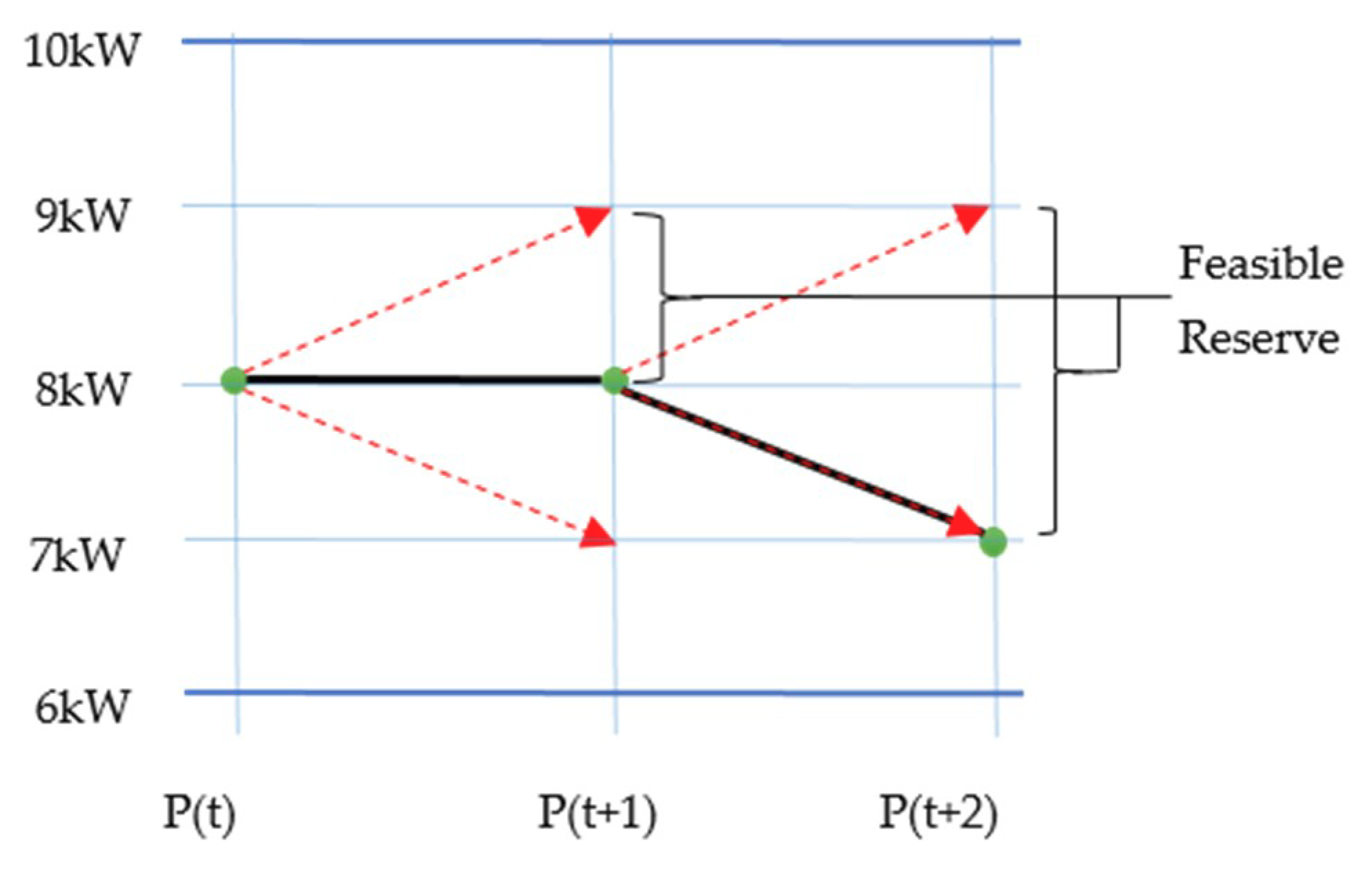
2.4.2. Feasible Generator Limits

The computation strategy for the diesel generator limits can be divided into three P_max resetting using Equations (13) and (14), considering the start-up and shut-down conditions, followed by the feasible generator boundaries calculation in Equation (17).

$$\begin{array}{l}U{B}_i\left(t\right)=\min \left(P_{DG,i}\left(t-1\right)+Rm{p}_{DG,i},P_{\max ,i}\right)\\ L{B}_i\left(t\right)=\max \left(P_{DG,i}\left(t-1\right)-Rm{p}_{DG,i},P_{\min ,i}\right)\end{array}.$$

(17)

2.5. Reserve Cases

There are three cases to be studied in this paper, each with varying treatments of the reserve consideration. All the cases use Equations (2)–(10), (13), (15), and (16).

Case 1: Conventional Reserve.

This case is the traditional computation of reserve for the DAUC. This scheme schedules a minimum reserve using the maximum and minimum generator limits. The RNS is computed using Equation (18), with the corresponding reserve constraint in Equation (11).

$$RNS={\displaystyle \sum _{t=1}^T{\displaystyle \sum _{i=1}^{ngen}U{C}_i\left(t\right)\left(P_{\max ,}{}_i\left(t\right)-P_{DG,i}\left(t\right)\right)-SR\left(t\right)}}.$$

(18)

Case 2: Feasible Reserve Strategy.

This case is the proposed computation for a feasible scheduled reserve in Equation (12) and requires the use of Equations (14) and (17) for the computation of the feasible limits. This means that the scheduled reserve only considers what is indeed available from the committed generators, and makes use of the ramp trajectories of the previous P_DG to the current time as the generator boundaries. The RNS for this case is computed using Equation (19).

$$RNS={\displaystyle \sum _{t=1}^T{\displaystyle \sum _{i=1}^{ngen}U{C}_i\left(t\right)\left(U{B}_i\left(t\right)-P_{DG,i}\left(t\right)\right)-SR\left(t\right)}}.$$

(19)

Case 3: Balance of Case 1 and Case 2.

Like Case 2, Case 3 still schedules the feasible scheduled reserve in Equation (12), including Equations (14) and (17), in the base case problem, but computes the RNS in Equation (18). This implies that, though the feasible scheduled reserve is required in the UC decision (first stage), the cost of the RNS is still allowed in the ED decision (second stage).

3. Partitioned Step Particle Swarm Optimization

Partitioned step PSO is a PSO variant that incorporates additional components which include adaptive components, crossover, and partitioning. The adaptive component is a modified form of adaptive PSO (APSO) in [28] and is combined with principles of partitioning harmonies similar to HS.

The theory of the adaptive component of APSO is to consider the characteristics of the current solution and its distance to the current global best. The inertia weight ω should be moved according to certain conditions. For the PSPSO, these conditions are formulated as the λ and γ components. The λ component tells the characteristic of the current set of solutions, and the larger the value the closer the solutions are. The γ component describes the distance of a particle to the current best solution; the larger the value, the nearer the particle is to the global best solution. Equation (20) shows the computation of the two components and their relation to ω for this algorithm.

$$\begin{array}{l}\lambda =f{x}_{\min }/f{x}_{\max }\\ \gamma =1-\frac{fx-gbest}{f{x}_{\max }-gbest}\\ \omega =\gamma \times \lambda \times (Iter-x)/Iter\end{array}.$$

(20)

At the beginning of the algorithm, when the fitness range is very large ω will be in the usual range of other PSOs. At this point, the algorithm will try to improve the solution by moving towards the pbest and gbest. When the particles suddenly try to converge (both λ and γ are high), ω will be higher than usual, thus the algorithm tries to search more space.

The traditional random walk for PSO includes the previous velocity, pbest, and gbest. Nonetheless, some research suggests that including gbest makes the algorithm converge prematurely [29,30,31]. However, for this paper, instead of removing gbest, the gbest will have a reduced effect on the velocity at the start of the iteration, then it gradually increases as the algorithm approaches the maximum iteration. The algorithm also considers the effect of other pbests in the direction of the particle. The variable a, called the partitioning variable, is used to identify which particles will be affected by gbest or pbest. The PSPSO step is found in Equation (21).

$$\begin{array}{l} a=rand<x/Iter\\ vel=\omega \times vel+c_1\times rand\times \left(pbest-part\right)\\ +c_2\times rand\times \left(a\times gbest+\left(1-a\right)\times pbest-part\right)\\ part=part+vel\end{array}.$$

(21)

4. Data and Results

This section is divided into two: the results of the UC cases and the robustness test result. As discussed in Section 2.5, all cases use Equations (2)–(10), (13), (15), and (16). Case 1 uses the reserve schedule of Equation (11) and an RNS of Equation (18). Case 2 uses Equations (14) and (17) for the feasible limit and Equations (12) and (19) for the reserve schedule and the RNS. Lastly, Case 3 also uses Equations (14) and (17) for the feasible limit and Equations (11) and (18) for the reserve schedule and the RNS. Furthermore, a 10% probability of repairing the power balance and time constraint in case there are constrain violations was used to add some randomness on the search. In this case, the best per unit cost priority list (BP-PL) in [12] is used to decide which generator to use in the repair.

4.1. Unit Commitment

The proposed PSPSO algorithm uses a c1 = c2 = 1.5 and a population of 50, which were determined through the prior optimization of the algorithm. The PSPSO was able to solve the standard UC problem with a total cost of 563,934.17 at an average CPU time of 3.57 sec. This UC is the same UC already found in the literature [11], with some discrepancy in the ED, making this paper’s total cost slightly lower than that of [8,9,10,11,12]. This means that the PSPSO is suitable for solving the UC problem.

The base case results (no PV) of the 10-unit UC with the additional constraints can be seen in Figure 4. These base case results also show the infeasible reserve of conventional computation in Figure 5. Notice that, at t = 20, it shows that all the generators are operating at their upper limit based on the ramping constraint. This means that, at this hour, the generators can no longer ramp up if there is a need for additional power. As also seen in Figure 5 at t = 20, the system sees that there is a reserve (red line) available, but the current set of generators is not capable of supplying this amount if required. This emphasizes the proposed feasible reserve.

4.1.1. Costs

From

Table 2. Day-ahead unit commitment cost of the three cases for different scenario considerations.

Case 1	no PV	mean PV	Number of PV Scenarios					Number of PV and Load Scenarios
			10	20	30	40	50	10 × 10	20 × 20	30 × 30	40 × 40	50 × 50
Fuel Cost	560,325	484,791	528,822	528,283	528,751	528,843	529,023	548,146	548,344	548,450	548,075	548,899
Start-Up	4090	4590	4040	4030	4030	4040	4040	4040	3310	4030	4040	3480
ENS	0	0	0	0	0	0	0	0	0	0	0	4
RES	0	0	0	0	0	0	0	0	0	0	0	62
Total	564,415	489,381	532,862	532,313	532,781	532,883	533,063	552,186	551,654	552,480	552,115	552,445
Case 2
Fuel Cost	573,017	495,047	534,354	535,891	535,596	535,776	537,189	552,396	553,589	552,742	553,493	553,087
Start-Up	3600	4430	4150	3050	2990	2990	2990	2990	2990	3050	2820	2990
ENS	0	0	0	0	0	0	0	0	0	0	0	0
RES	0	0	0	0	0	166	192	16	40	45	307	89
Total	576,617	499,477	538,504	538,941	538,586	538,932	540,371	555,402	556,619	555,837	556,620	556,167
% of C1*	2.16%	2.06%	1.06%	1.24%	1.09%	1.14%	1.37%	0.58%	0.90%	0.61%	0.82%	0.67%
Case 3
Fuel Cost	573,667	494,791	534,674	535,104	534,807	535,420	533,803	551,789	550,516	552,264	552,176	552,377
Start-Up	3600	3540	3540	2990	2990	3540	4090	3280	3830	3540	2990	2990
ENS	0	0	0	0	0	0	0	0	0	0	0	0
RES	0	0	0	0	0	0	0	0	0	0	0	0
Total	577,267	498,331	538,214	538,094	537,797	538,960	537,893	555,069	554,346	555,804	555,166	555,367
% of C1*	2.28%	1.83%	1.00%	1.09%	0.94%	1.14%	0.91%	0.52%	0.49%	0.60%	0.55%	0.53%

* % of C1 indicates the increase in case 2 or case 3 cost compared to the cost in case 1 with the same scenario consideration.

, case 2 always has the highest cost. This, however, just increases the DA costs as compared to case 1 by 2.16% for no PV and 2.06% for mean PV (single scenario). Case 3, on the other hand, increases the cost compared to case 1 to 2.28% for no PV and 1.83% for a mean PV (single scenario). When the scenarios are considered, the increase from case 1 to case 2 and case 3 costs is much lesser, no more than 1.24% when considering the PV uncertainties, and no more than 0.9% when considering the uncertainties from both PV and load. It is also evident that an increase in cost is much lesser when considering scenarios from both PV and load than when considering just scenarios from PV. This means that, when considering more sources of uncertainties, the three cases would account for almost the same costs to adjust to the same scenario set.

Table 2 also shows that case 2 usually has the highest cost, followed by case 3, and then case 1. This clearly shows that case 3 is the compromised condition of case 1 and 2. Additionally, there is a remarkable increase in cost from considering the 1 scenario to 10 scenarios in all of the cases. This implies that protecting the system from uncertainties increases the operational cost. Furthermore, this increase is not larger than the cost of the system without renewable energy. Thus, in any case, adding the PV still makes the system decrease its operational costs.

4.1.2. Losses

The ENS and the RNS are the two losses considered in the operational cost. Table 2 shows the breakdown of the operational costs. This table shows that there are hardly any ENS or RNS when only PV scenarios are considered. The ENS and RNS increase when more sources of uncertainties, PV, and load are considered in the system. Additionally, for the results of case 2, more RNS are expected because the consideration of the reserve is rather constricted compared to the other cases. Nonetheless, no load shedding occurred.

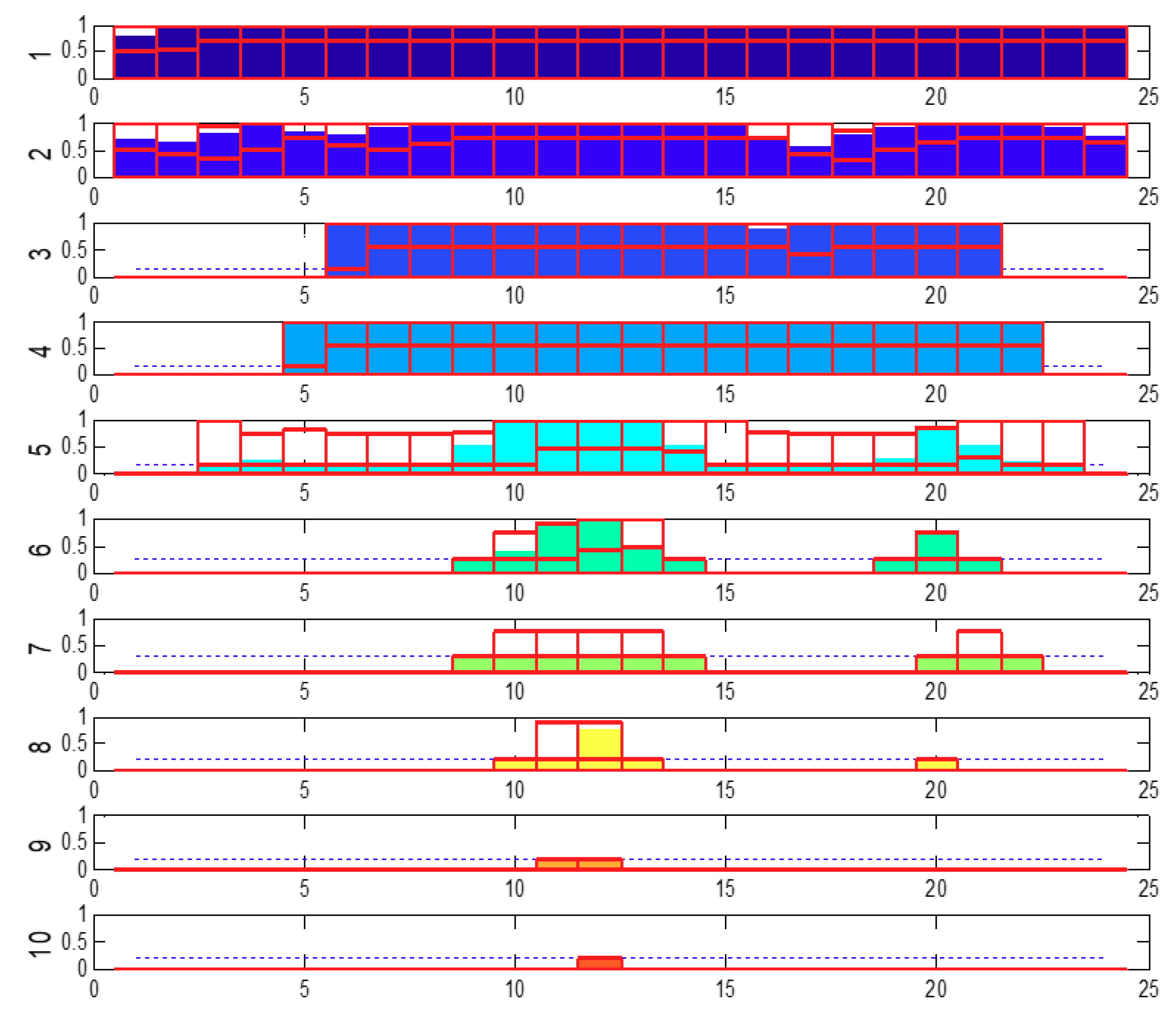
4.1.3. Committed Units

For all three cases, increasing the number of sources of uncertainties mostly increases the number of generator hours. This can be seen in the lower start-up costs and higher fuel costs in Table 2 for case 2 and case 3.

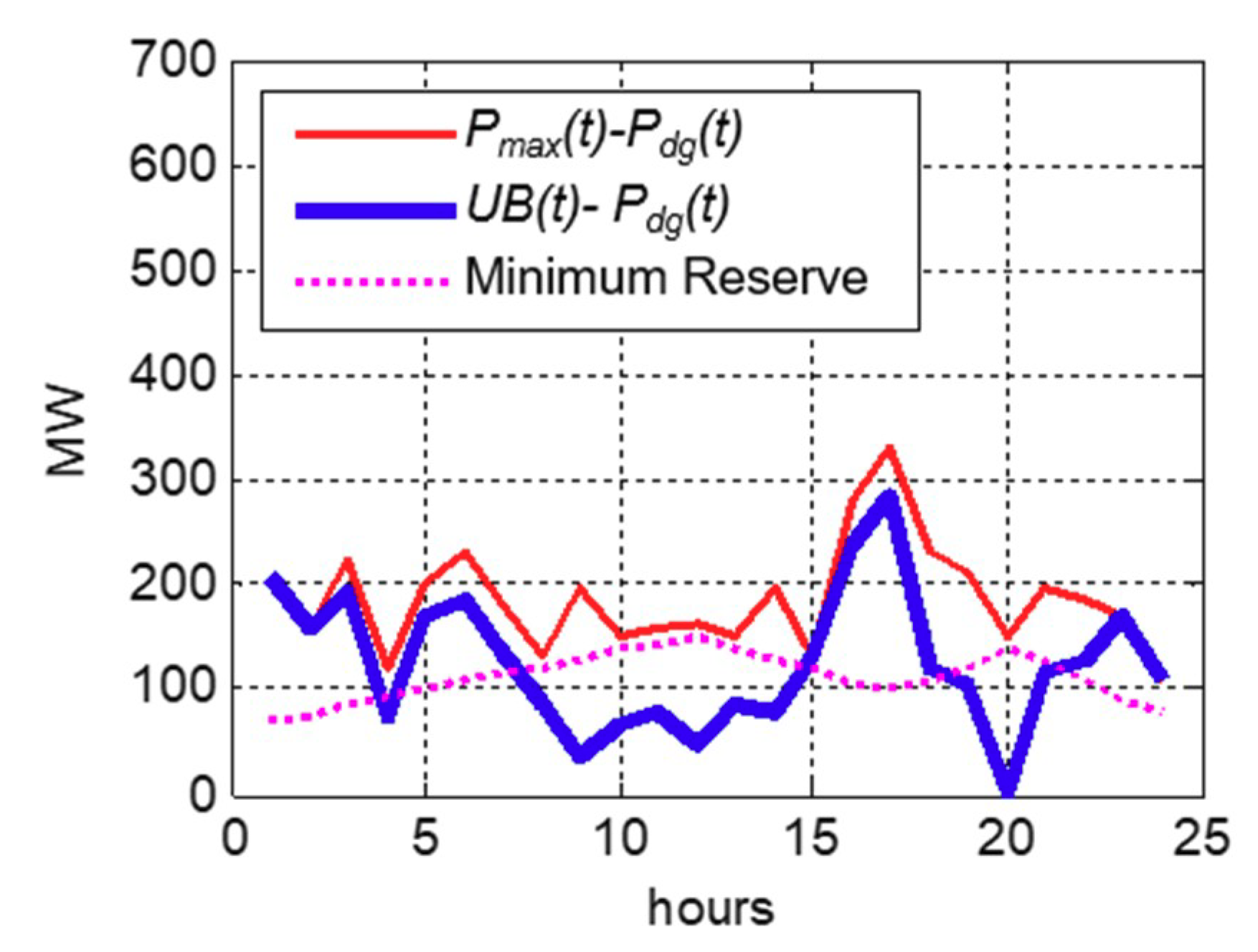
4.1.4. Hourly Reserve

Figure 6 shows the difference in the feasible reserve schedule and the minimum reserve considering the PV uncertainty (left column) and PV load uncertainty (right column) for the three cases. Note that the difference between the conventional reserve computation and the minimum reserve does not result in any minimum reserve constraint violation for all the three cases.

In case 1, the first row of Figure 6, there is a lot of reserve violation because it does not consider if the set UC can indeed increase up to maximum value when needed, given the characteristics of the generators. There is a lot of reserve violations at the hours where some generators have just started—at hours 4, 6, and 20—where there are reserve violations for the scenario cases. Case 2 and 3, on the other hand, have no minimum reserve violation for feasible reserve. Cases 2 and 3 were able to prepare to increase the system capacity given the capability of the online generators, and were able to turn on some generators ahead to maintain the minimum reserve at the same hours. Case 1 has some reserve violations.

In general, case 2 schedules the highest reserve compared to case 3 and case 1, as this case considers the feasible reserve in both the UC and ED decisions. Meanwhile, in Case 3 there are more points where the reserve schedule is very near the minimum reserve, because it only considers the feasible reserve in the UC decision.

Increasing the number of scenarios does not provide much change in the cost, UC, and reserve. Additionally, considering more sources of uncertainty generally increases the total reserve schedule in the majority of the cases, as shown in Figure 7. On the contrary, more sources of uncertainty decrease the hourly reserve schedule around the peak hours, as seen in the change from left (PV scenarios) to right (PV and load scenarios) in Figure 6. It may be possible that the consideration of both uncertainties from PV and load somehow compensates for each other, making the reserve schedule a little bit flatter than considering only PV uncertainties.

The increase in the reserve schedule from case 1 to case 2 and from case 1 to case 3, in Figure 7, average around 20% and 15%, respectively. This increase does not necessarily mean that the increase is throughout the period, as seen in Figure 6. Figure 7 also implies that there is a huge difference in the computation of the feasible reserve and the conventional reserve computation, and this may have an impact on adapting to uncertainty, as will be tested in the next section.

4.2. Test for Robustness

In this last section, the UC is tested on how well the computation has prepared the system for uncertainties. The initial generated set of scenarios were reclassified into four: low uncertainty, moderate uncertainty, moderate-high uncertainty, and high uncertainty. After the reclassification, a representative of each group is chosen as a test scenario for the UC results. The OTD operational cost, Equation (1), is again recalculated using each of the four scenarios. The results are shown in

Table 3. Day-ahead and on-the-day costs.

UC Method and Reserve Case	DA Cost	OTD Cost					% Increase in Costs
		Fuel	SU	ENS	RNS	Total
High Uncertainties
DUC-C1	489,380	544,232	4590	448,000	403,700	1,400,522	186.18%
DUC-C2	499,477	551,569	4430	10,500	124,300	690,799	38.30%
DUC-C3	498,330	551,122	3540	10,500	124,300	689,462	38.35%
SUC-C1-PV	532,861	550,137	4040	0	0	554,177	4.00%
SUC-C2-PV	538,504	552,585	4150	0	0	556,735	3.39%
SUC-C3-PV	538,214	554,131	3540	0	0	557,671	3.62%
SUC-C1-PVL	552,186	548,755	4040	0	0	552,795	0.11%
SUC-C2-PVL	555,401	552,724	2990	0	0	555,714	0.06%
SUC-C3-PVL	555,068	552,020	3280	0	0	555,300	0.04%
Medium-High Uncertainties
DUC-C1	489,380	542,182	4590	696,500	279,400	1,522,672	211.14%
DUC-C2	499,477	550,013	4430	0	143,000	697,443	39.63%
DUC-C3	498,330	550,595	3540	0	143,000	697,135	39.89%
SUC-C1-PV	532,861	548,940	4040	0	0	552,980	3.78%
SUC-C2-PV	538,504	551,584	4150	0	0	555,734	3.20%
SUC-C3-PV	538,214	553,371	3540	0	0	556,911	3.47%
SUC-C1-PVL	552,186	548,000	4040	0	0	552,040	−0.03%
SUC-C2-PVL	555,401	551,322	2990	0	0	554,312	−0.20%
SUC-C3-PVL	555,068	550,866	3280	0	0	554,146	−0.17%
Medium Uncertainties
DUC-C1	489,380	543,424	4590	0	172,700	720,714	47.27%
DUC-C2	499,477	547,659	4430	0	0	552,089	10.53%
DUC-C3	498,330	548,125	3540	0	0	551,665	10.70%
SUC-C1-PV	532,861	546,253	4040	0	0	550,293	3.27%
SUC-C2-PV	538,504	549,942	4150	0	0	554,092	2.89%
SUC-C3-PV	538,214	551,370	3540	0	0	554,910	3.10%
SUC-C1-PVL	552,186	544,757	4040	0	0	548,797	−0.61%
SUC-C2-PVL	555,401	549,636	2990	0	0	552,626	−0.50%
SUC-C3-PVL	555,069	548,996	3280	0	0	552,276	−0.50%
Low Uncertainties
DUC-C1	489,380	540,796	4590	0	40,700	586,086	19.76%
DUC-C2	499,477	545,330	4430	0	0	549,760	10.07%
DUC-C3	498,330	544,911	3540	0	16,500	564,951	13.37%
SUC-C1-PV	532,861	544,201	4040	0	0	548,241	2.89%
SUC-C2-PV	538,504	546,749	4150	0	0	550,899	2.30%
SUC-C3-PV	538,214	548,243	3540	0	0	551,783	2.52%
SUC-C1-PVL	552,186	541,983	4040	0	0	546,023	−1.12%
SUC-C2-PVL	555,401	546,179	2990	0	0	549,169	−1.12%
SUC-C3-PVL	555,068	545,747	3280	0	0	549,027	−1.09%

. The increase in the cost from the DA planning to the OTD operation is likewise computed.

4.2.1. Deterministic Cases

The results show that, for the deterministic cases, considering the feasible reserve improves the robustness of the system in adapting to uncertainty. As seen in Table 3, case 1 always has the largest increase in cost due to the large ENS and RNS, which increase the cost from 19.76% to 211.14% of its DA cost. Case 2 and case 3 show a comparatively low increase in costs compared to case 1, with the ENS costs only in the high-uncertainty set. Case 3 almost performs the same as case 2, except for the last scenario pair, where it has some RNS but not as much as in case 1. Finally, case 2 always has the lowest increase in costs because the ENS and RNS are also the lowest. Therefore, for the deterministic approach, case 2 clearly shows the best reserve scheduling and can robustly adapt to the uncertainties.

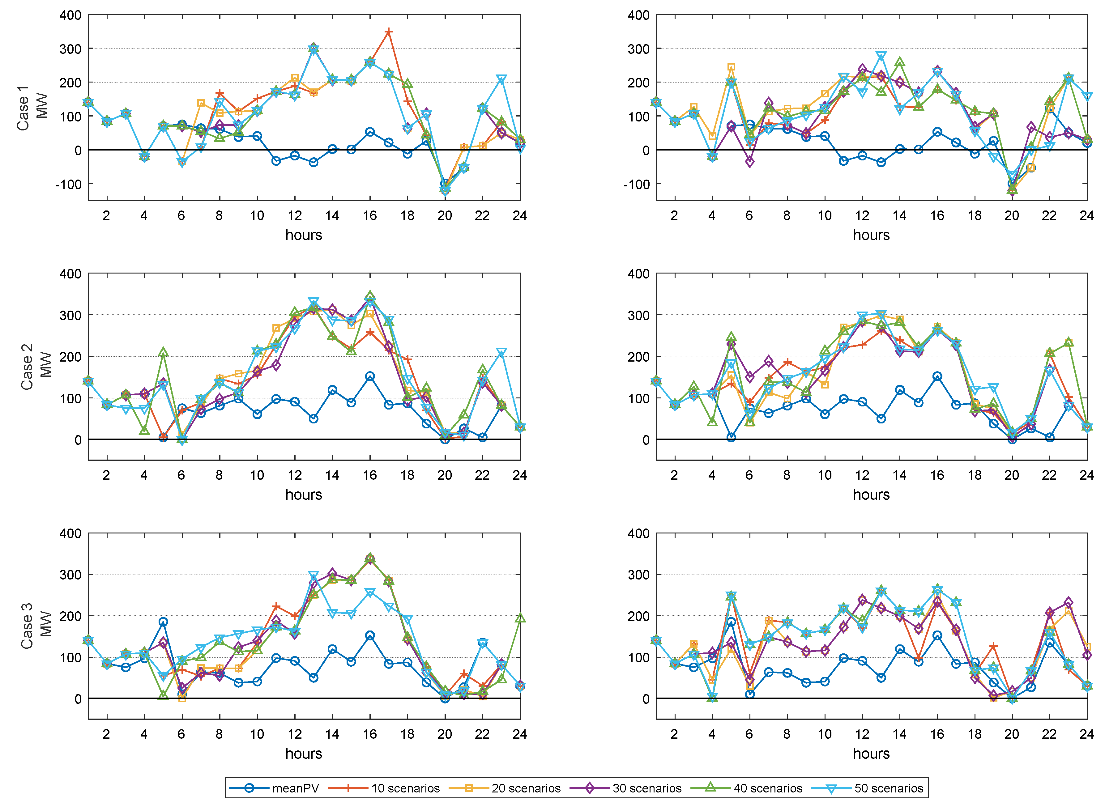
4.2.2. Scenario-Based Cases

For all cases of scenario-based approaches, the increase in cost is not high compared to the deterministic cases. This shows that the scenario-based approach better prepares the system against large uncertainties, where case 2 usually shows the lowest increase in the cost of all the cases, indicating that case 2 can better prepare the system for uncertainties. On the other hand, when considering more sources of uncertainties, there are relatively lower increases or decreases (shown by the negative sign) in cost for all cases. Both cases 2 and 3 usually have a near-zero increase, implying that they have better accuracy in predicting the OTD cost and operation. It is also important to note that, as found in the literature, when more sources of scenarios are considered, the computational time increases exponentially.

5. Discussion

The PSPSO was able to perform well to solve the unit commitment problem compared with what is found in the literature. Although the algorithm may be effective for this problem, tests may still be conducted if the algorithm may be effective in another type of problem. However, for the UC problem, the average speeds in the deterministic case, PV scenario cases, and PV-load scenario cases are 20.29 seconds, 1.14 minutes, and 10.37 minutes, respectively, for the entire 1000 iterations, which is an adequate time for day-ahead or on-the-day decisions to be made. Note that these results were done in an Intel Core i5-6500 CPU at 3.2 GHz. Changing the termination criteria or having better computational power would decrease the decision time.

The feasible reserve approach proposed in this paper presents a single UC decision which can handle the uncertainty from both the renewable source and the load. Most stochastic optimization in the literature does not provide a UC decision, but rather just a prediction of the possible operational cost, giving different possible UCs that may be used for different levels of uncertainty or different scenarios. This can be seen in how the other studies wrote their objective equation, where the SU costs depend on a certain probability, as compared to Equation (2), in this paper.

The UC decision method proposed by this paper is a robust UC decision in handling high levels of uncertainty by considering the feasible reserve. The results have shown that consideration of the feasible reserve indeed is important on the base UC problem, even with the deterministic approach, where the feasible reserve has a compelling benefit when comparing the DA costs with the OTD cost compared with the conventional UC approach (case 1). The traditional UC problem still has load curtailment in high to medium-high uncertainty, and reserve penalty on all levels of uncertainty. Meanwhile, as for the feasible reserve deterministic approaches, load curtailment was only done on a high level of uncertainty. Though the deterministic approaches are much faster, the scenario-based cases provide a more robust solution, with case 2 being the most robust.

The feasible reserve method proposed in this paper can be used as a decision-making tool for DAUC and also for the ED decisions for OTD operations. The method itself can be programmed as a software tool for system operators in deciding the DAUC. Once the UC is already set for OTD operation, the feasible generator limits and feasible reserve strategies can be incorporated in the ED scheduling of generators and later on can be used as inputs to its controls.

Not covered in this paper is the prediction PV output. The paper only used a generalized uncertainty model considering the percent increase or decrease in solar irradiance. In this regard, improvement can be made by either predicting the maximum and minimum decrease in irradiance or the time-series of minimum, maximum, and mean irradiance for the next day or current day.

6. Conclusions

The proposed methods, case 2 and case 3, have a clearer view of what the system’s real capability is and can prepare the system for uncertainties by providing the required reserve (from the scheduling of UC and ED) and scheduling the PV to avoid any losses. The two methods, especially case 2, exhibit remarkable robustness in the deterministic case compared to the deterministic conventional method. For scenario-based cases, the proposed method’s performance in coping with the different levels of uncertainty is almost the same but better than the conventional method.

Although the performance of the three cases is quite the same in the scenario-based approach, the advantage of using the proposed methods may be seen in the accuracy of predicting the OTD costs and operation using the DAUC. Having large discrepancies in the DA cost and OTD cost may incur some losses to the power producer.

In summary, the proposed methods do provide a higher DA cost compared with the conventional method, but can effectively make the system more flexible by making sure that the available reserve is indeed available for use. Despite having more committed units and more reserve than the conventional method, the proposed method does not constitute a large increase in cost, especially when considering more sources of uncertainty.

References

1. Solar, Wind Power Generation Hits New High in Taiwan. Taiwan Today. 17 April 2018. Available online: https://taiwantoday.tw/news.php?unit=6&post=132786 (accessed on 17 April 2018).
2. Lee, A.H.I.; Chen, H.H.; Chen, J. Building smart grid to power the next century in Taiwan. Renew. Sustain. Energy Rev. 2017, 68, 126–135. [Google Scholar] [CrossRef]
3. Ngitevelekwa, K.; Bansal, R. A review of generation dispatch with large-scale photovoltaic systems. Renew. Sustain. Energy Rev. 2018, 81, 615–624. [Google Scholar] [CrossRef]
4. Notton, G.; Nivet, M.L.; Voyant, C.; Paoli, C.; Darras, C.; Motte, F.; Fouilloy, A. Intermittent and stochastic character of renewable energy sources: Consequences, cost of intermittence and benefit of forecasting. Renew. Sustain. Energy Rev. 2018, 87, 96–105. [Google Scholar] [CrossRef]
5. Lappalainen, K.; Valkealahti, S. Output power variation of different PV array configurations during irradiance transitions caused by moving clouds. Appl. Energy 2017, 190, 902–910. [Google Scholar] [CrossRef]
6. Abujarad, S.; Mustafa, M.; Jamian, J. Recent approaches of unit commitment in the presence of intermittent renewable energy resources: A review. Renew. Sustain. Energy Rev. 2017, 70, 215–223. [Google Scholar] [CrossRef]
7. Theo, W.L.; Lim, J.S.; Ho, W.S.; Hashim, H.; Lee, C.T. Review of distributed generation(DG) system planning and optimization techniques: Comparison of numerical and mathematical modelling methods. Renew. Sustain. Energy Rev. 2017, 67, 531–573. [Google Scholar] [CrossRef]
8. Saber, N.A.; Salimi, M.; Mirabbasi, D. A priority list based approach for solving thermal unit commitment problem with novel hybrid genetic-imperialist competitive algorithm. Energy 2016, 117, 272–280. [Google Scholar] [CrossRef]
9. Srikanth, K.; Panwar, L.K.; Panigrahi, B.K.; Herrera-Viedma, E.; Sangaiah, A.K.; Wang, G.G. Meta-heuristic framework: Quantum inspired binary grey wolf optimizer for unit commitment problem. Comput. Electr. Eng. 2017, 70, 243–260. [Google Scholar] [CrossRef]
10. Panwar, L.; Reddy, S.; Verma, A.; Panigrahi, B.K.; Kumar, R. Binary grey wolf optimizer for large scale unit commitment problem. Swarm Evol. Comput. 2018, 38, 251–266. [Google Scholar] [CrossRef]
11. Quan, H.; Srinivasan, D.; Khosravi, A. Integration of renewable generation uncertainties into stochastic unit commitment considering reserve and risk: A comparative study. Energy 2016, 103, 735–745. [Google Scholar] [CrossRef]
12. Shukla, A.; Singh, S. Multi-objective unit commitment with renewable energy using hybrid approach. IET Renew. Power Gener. 2016, 3, 327–338. [Google Scholar] [CrossRef]
13. Hedayati-Mehdiabadi, M.; Hedman, K.; Zhang, J. Reserve Policy Optimization for scheduling wind energy and reserve. IEEE Trans. Power Syst. 2018, 1, 19–31. [Google Scholar] [CrossRef]
14. Soltani, Z.; Ghaljehei, M.; Gharehpetian, G.B.; Aalami, H.A. Integration of smart grid technologies in stochastic multi-objective unit commitment: An economic emission analysis. Int. J. Electr. Power Energy Syst. 2018, 100, 565–590. [Google Scholar] [CrossRef]
15. Ye, H.; Wang, J.; Ge, Y.; Li, J.; Li, Z. Robust integration of high-level dispatchable renewables in power system operation. IEEE Trans. Sustain. Energy 2017, 2, 826–835. [Google Scholar] [CrossRef]
16. Pandzic, H.; Dvorkin, Y.; Qiu, T.; Wang, Y.; Kirschen, D.S. Toward cost-efficient and reliable unit commitment under uncertainty. IEEE Trans. Power Syst. 2016, 2, 970–981. [Google Scholar] [CrossRef]
17. Zhang, Y.; Wang, J.; Ding, T.; Wang, X. Conditional value at risk-based stochastic unit commitment considering the uncertainty of wind power generation. IET Gener. Trans. Distrib. 2018, 2, 482–489. [Google Scholar] [CrossRef]
18. Zhang, Y.; Wang, J.; Zeng, B.; Hu, Z. Chance-Constrained Two-stage Unit Commitment under uncertain Load and Wind Power Output Using Bilinear Benders Decomposition. IEEE Trans. Power Syst. 2017, 5, 3637–3647. [Google Scholar] [CrossRef] [Green Version]
19. Shi, Z.; Liang, H.; Dinavahi, V. Data-driven distributionally robust chance-constrained unit commitment with uncertain wind power. IEEE Access 2019, 7, 135087–135098. [Google Scholar] [CrossRef]
20. Shao, C.; Wang, X.; Shahidehpour, M.; Wang, X.; Wang, B. Security-constrained unit commitment with flexible uncertainty set for variable wind power. IEEE Trans. Sustain. Energy 2017, 3, 1237–1246. [Google Scholar] [CrossRef]
21. Khatami, R.; Parvania, M.; Narayan, A. Flexibility reserve in power systems: Definition and stochastic multi-fidelity optimization. IEEE Trans. Smart Grid 2019, 11, 644–654. [Google Scholar] [CrossRef]
22. Alizadeh, M.I.; Moghaddam, M.P.; Amjady, N. Multistage multiresolution robust unit commitment with nondeterministic flexible ramp considering load and wind variables. IEEE Trans. Sustain. Energy 2018, 2, 872–883. [Google Scholar] [CrossRef]
23. Parvania, M.; Scaglione, A. Unit commitment with continuous-time generation and ramping trajectory models. IEEE Trans. Power Syst. 2016, 4, 3169–3178. [Google Scholar] [CrossRef]
24. Khatami, R.; Parvania, M. Continuous-time locational marginal price of energy. IEEE Access 2019, 7, 129480–129493. [Google Scholar] [CrossRef]
25. Blanco, I.; Morales, J. An efficient robust solution to the two-stage stochastic unit commitment problem. IEEE Trans. Power Syst. 2017, 6, 4477–4488. [Google Scholar] [CrossRef] [Green Version]
26. Bruninx, K.; Delarue, E. Endogenous probabilistic reserve sizing and allocation in unit commitment models: Cost effective, reliable and fast. IEEE Trans. Power Syst. 2017, 4, 2593–2603. [Google Scholar] [CrossRef]
27. NASA. Surface Meteorology and Solar Energy. Available online: https//eosweb.larc.nasa.gov/cgi-bin/sse/retscreen.cgi?email=skip%40larc.nasa.gov&step=1&lat=24.77&lon=121.04&submit=Submit (accessed on January 2018).
28. Han, H.-G.; Lu, W.; Hou, Y.; Qiao, J.-F. An Adaptive-PSO-Based Self-Organizing RBF Neural Network. IEEE Trans. Neural Netw. Learn. Syst. 2018, 29, 104–117. [Google Scholar] [CrossRef] [PubMed]
29. Bonyadi, M.R.; Michalewicz, Z. Analysis of stability, local convergence, and transformation sensitivity of a variant of the particle swarm optimization algorithm. IEEE Trans. Evol. Comput. 2016, 3, 370–385. [Google Scholar] [CrossRef] [Green Version]
30. Liang, J.J.; Qin, A.K.; Suganthan, P.N.; Baskar, S. Comprehensive learning particle swarm optimizer for global optimization of multimodal functions. IEEE Trans. Evol. Comput. 2006, 3, 281–295. [Google Scholar] [CrossRef]
31. Li, Y.; Zhan, Z.H.; Lin, S.; Zhang, J.; Luo, X. Competitive and cooperative particle swarm optimization with information sharing mechanism for global optimization problems. Inf. Sci. 2015, 293, 370–382. [Google Scholar] [CrossRef]
Figure 1. Feasible reserve capability of generators due to ramping up and down.
Energies 13 05239 g001
Figure 2. Solar irradiance: (a) monthly mean (1983–2005) in per unit from NASA-SSE and (b) the hourly irradiance per month in the per unit value.
Energies 13 05239 g002
Figure 3. Clustered (a) PV output scenarios and (b) load profile scenarios; reduced (c) PV output scenarios and (d) load profile scenarios.
Energies 13 05239 g003
Figure 4. Unit commitment and load factor of the 10-unit problem for case 1.
Energies 13 05239 g004
Figure 5. Conventional reserve and feasible reserve of the deterministic case 1.
Energies 13 05239 g005
Figure 6. Difference between the feasible reserve schedule and minimum reserve from the results considering PV scenarios (left column) and PV load scenarios (right column) for cases 1, 2, and 3 (top to bottom).
Energies 13 05239 g006
Figure 7. Total (a) feasible reserve and (b) conventional reserve for every increase in scenarios for cases 1, 2, and 3.
Energies 13 05239 g007