1. Introduction
Vehicle integrated thermal management system (VTMS) technologies have demonstrated their potential in a variety of fields, including powertrains, electrical systems such as motors and batteries, passenger comfort systems, and implementation of new powertrain technologies and emission control systems [
1,
2]. Among the numerous technologies related to improving fuel economy, when efficiency and improvement in fuel economy are considered compared to the increase in production cost of a vehicle, VTMS technologies are expected to cost less than
$50 per 1% reduction in fuel consumption [
3]; therefore, automakers are showing significant interest in the technology and are actively applying it to their products [
4].
Despite the interests of manufacturers and the demands of the market, there are several challenges in the application of this technology. For optimal operation of VTMS, it is necessary to analyze and predict the system behavior. However, adding sensors for system behavior analysis increases the cost. Therefore, manufacturers use several methods to minimize the number of sensors required. For example, CFD-based analysis for prediction [
5,
6], simplified model-based prediction [
7,
8], and model-based analysis for optimization by relocating the sensor [
9] have been utilized.
Modeling a thermal management system requires considerable time for experimental parameter studies, as well as manpower in various fields, such as heat transfer, combustion engineering, and fluid mechanics, to construct the model and expensive systems such as environmental chambers. This trend will become more complex with the gradual evolution of thermal management systems.
The vehicle’s control system requires a heavy software. Passenger vehicles use four times as many lines of code as a commercial aircraft [
10]. Software development costs have gradually increased and have risen to the same level as hardware development costs [
11]. While model-based software development is being implemented to reduce development time and cost [
3], automakers are still looking for opportunities to increase the flexibility of their workforce or gradually reduce the use of their own resources [
12,
13]. Along with this trend, there is a need for a simplified development method that can further reduce time, manpower, and costs from conventional thermal management system modeling techniques.
The physics-based method is conventionally used for predicting the energy flow. However, it requires several experimental approaches to obtain the required parameters; thus, the cost is high. Neural networks have been proposed to address this limitation of physics-based modeling.
Instead of figuring out the laws of physics as in the physics-based prediction method, the neural network (NN) method determines the causal relationship between the input and the output. Hence, the intermediate experimental parameter study processes can be omitted. The NN method has excellent generalization performance and shows robust results even with noisy or incomplete data, and is also durable against model defects [
14,
15,
16,
17]. Since the NN method has many processing nodes, defects in several nodes or connections do not cause serious defects in the entire system [
18,
19]. Therefore, it is suitable for complex models with many variables and auto-regression problems [
20]. It can also be a powerful solution to the problem of coupling data with a variety of inputs [
21].
VTMS modeling can be defined as a multivariate time series forecasting problem. Traditionally, time series prediction has been dominated by linear methods such as autoregressive integrated moving average (ARIMA) and vector auto-regression (VAR), which are intuitive for variant problems [
22]. However, these classical methods have several limitations, such as problems when data are missing or corrupted and difficulties with multi-step prediction [
23]. Furthermore, they predict from a linear relationship to a generalized relationship rather than a complex relationship and, because of the temporal dependence problem, it is necessary to diagnose and specify the number of delayed observations.
Multilayer perceptron (MLP) can overcome some of the disadvantages of ARIMA and VAR. The same simple neural network approximates a mapping function from an input variable to an output variable. This general capability is useful for time series because it can solve various problems such as noise, non-linearity, multivariate input, multi-step inputs, and lack of robustness. Feedforward neural networks do offer great capability but still have the limitation of having to specify the temporal dependence during the model design step [
24].
In recent time series prediction research, several studies have proposed variants of recurrent neural network (RNN) and convolutional neural network (CNN) [
25]. CNN learns by automatically extracting features from raw data using a method known as expression learning. CNN guarantees shift and distortion invariance with local acceptance, shared or replication weight, and spatial and temporal subsampling [
26,
27]. These CNN characteristics are useful for preprocessing in time series prediction [
28].
RNN is a dedicated sequence model that keeps hidden activation vectors propagating through time [
27] (pp. 3–7). Long short-term memory (LSTM), a variant of RNN, explicitly handles the ordering between observations when learning the input-to-output mapping function not provided by MLP or CNN. LSTM natively supports sequences and the persistence of state can learn temporal dependence. LSTM networks eliminate the need for predefined time windows and can accurately model complex multivariate sequences [
29].
The most recent studies present a modified architecture of RNNs and CNNs. Convolutional long short-term memory (ConvLSTM) was developed for reading two-dimensional spatial-temporal data [
30], but it can be adapted for use with multivariate time series forecasting [
27] (pp. 367–393). Temporal convolutional network (TCN) is more robust in learning and memory conservation than reference iterative architectures such as LSTM, GRU, and RNN in a wide range of sequence modeling tasks [
31]. TCN is an architecture that was developed for video-based action segmentation in 2017 [
32] and the scope of its application has started to expand recently. The tasks in which it has been applied so far have been limited to areas such as traffic flow forecasting [
31], the text to speech (TTS) field represented by Google Deepmind’s Wavenet architecture [
33], and a wide range of areas with variant transform models.
Although time series forecasting for temperature using NNs is widely used in many other fields, attempts to approach NNs are rare in the VTMS field. The reason for this is that several VTMS devices are being applied to commercial vehicles in recent years and are still expanding [
34], and the existing physics-based modeling has not yet emphasized the need for other methods. Most of the NN studies are only partially applied to the state of charge [
35,
36] or temperature-related studies [
37] of battery electric vehicles (BEVs), and their application to other VTMS fields such as cooling system has not been considered.
In this study, the cooling system of a 1 L class gasoline vehicle equipped with an electric control valve (ECV) was modeled using physics-based modeling and NN approach, and the prediction results were compared. Through this comparison, we validate the applicability of NN modeling.
2. Physics-Based Modeling
There are various methods of physics-based modeling. We use the model-based method, a simplified model that can be embedded in a controller for establishing a control strategy or for model-based predictive control.
2.1. Model Structure
In this study, a small 1 L gasoline vehicle with separate cooling was selected as the target vehicle.
Table 1 is a brief specification of the vehicle used in the study. The manual transmission vehicle is equipped with a 98 horsepower gasoline engine, mechanical thermostat, and mechanical coolant pump. However, the mechanical thermostat was replaced with an ECV.
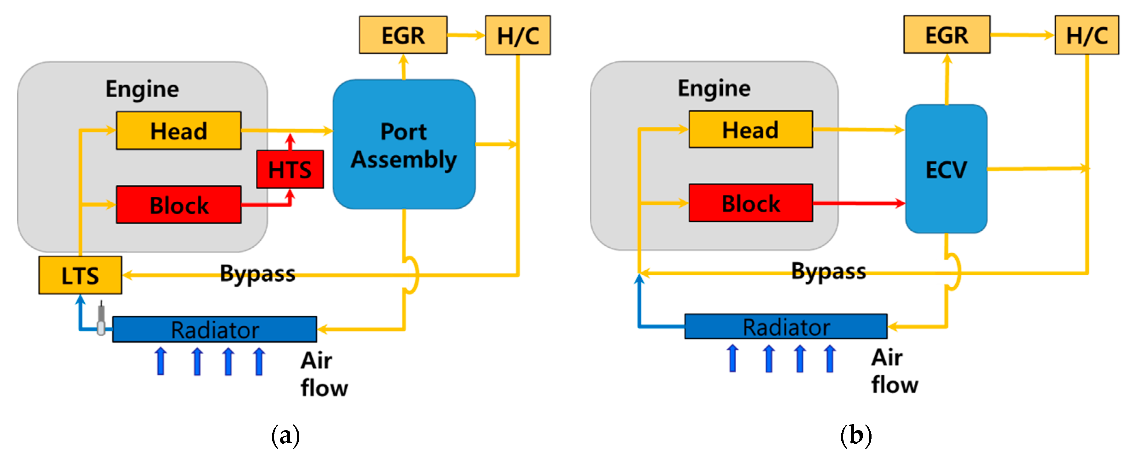
ECV is an electrically operated valve that replaces the thermostat to measure the temperature and ensure coolant flow to the desired part. Because mechanical thermostats operate only at a set temperature by opening the valve using the force of the expansion of the wax inside, we used ECV that can variably determine the coolant flow rate according to the desired control temperature and strategy.
Figure 1 shows the schematic of the vehicle cooling system used in this study. The cooling system of a car works as follows. The heat generated by fuel combustion in the engine is cooled by the radiator to keep the engine oil at a high temperature to maintain optimum viscosity. It also regulates the coolant temperature to optimize the operation of emission control devices such as exhaust gas recirculation (EGR). The coolant from EGR is then passed through the heater core (H/C) to heat the air supplied to the vehicle interior, because the heating, ventilation, and air conditioning (HVAC) was not operated, and the influencing factor was ignored in this study.
HVAC is based on the premise that it does not work according to regulations in mode tests (FTP-75, HWFET, WLTC) to measure fuel economy. Therefore, the mode results used in the verification data in this study are not related to the HVAC operation.
The vehicle used in this study has a manual transmission system. In general, manual transmissions do not have a heat exchanger for oil transmission so that modeling can be done in terms of coolant and engine oil.
According to previous studies, energy in vehicles is distributed as follows: About 25–28% of the heat generated inside the engine is transferred to power the spark ignition engine; 17–26% is transferred to the cooling system, and 3–10% in cooling the heat rejected or convection with oil. The rest is exhausted in the form of thermal energy or kinetic energy through the exhaust or converted into enthalpy loss [
38]. This is expressed as an energy balance equation as follows:
Here the expression on the left refers to the energy generated by the fuel combustion. is the combustion efficiency of fuel; is the fuel consumption; is the low heating value of gasoline. The expression on the right refers to the energy conversion into engine heat transfer rate to the coolant , brake power , exhaust energy loss , engine oil heat transfer , and other minor miscellaneous losses .
2.1.1. Engine Oil Temperature
The engine oil bulk temperature in oil pan can be simulated by the effect of heat generated inside the engine by fuel combustion (
, heat exchange with coolant to cool it at engine oil cooler (
, and heat exchange with ambient at oil pan and oil filter (
. The energy flow in the engine oil can be expressed as an energy balance equation as follows:
Each factor in Equation (2) is expressed in detail by the heat transfer equation as follows:
Some of the heat generated by combustion and mechanical friction in the cylinder contributes to the temperature rise in the coolant and engine oil. The amount of heat transferred by combustion inside the engine, which is a turbulent flow, should be analyzed for combustion. Rather than a complicated analysis, it is assumed that the ratio of the transfer function
due to engine heat generation
contributes to the temperature rise in coolant and engine oil, according to Equation (1) [
39].
To use Equation (3), both the inlet/outlet temperature when passing through the heat exchanger (engine oil cooler) must be known, but this measurement is difficult under actual conditions. Therefore, in this study, the model was modified using the Effectiveness-NTU method, which expresses effectiveness
as
Equation (3) can be expressed as follows by Equation (4).
2.1.2. Coolant Temperature
The behavior of coolant temperature is similar to that of engine oil but is more complex due to the influence of ECV, radiator, and bypass. However, when several variables are considered, the parameter determination becomes very complex and difficult; thus, the factors with minority influence were ignored. As shown in Equation (2), the factors that affect the coolant temperature can be expressed as:
One of the most difficult parts in expressing the coolant temperature behavior is expressing the heat exchanger of the radiator. The radiator can be expressed using the NTU-effectiveness method, similar to a general heat exchanger, but it is difficult to measure the coolant and ambient flow rate. The effectiveness of the radiator
expressed in Equation (4), can also be expressed as a function of temperature because the ambient temperature is colder than the coolant temperature.
The coolant flow rate is affected by the ECV’s opening area in the radiator direction and the operating speed of the water pump (
. Since the water pump is directly connected to the engine’s shaft, its operation is proportional to the engine speed (
. The opening area on the radiator side of the ECV (
is proportional to the defined valve shape and angle of the ECV motor
) which is an actuator that operates the valve. Therefore, the flow rate of coolant can be expressed as a function of the ECV’s operating angle and engine speed.
The flow rate of air reaching the front of the radiator can be expressed as the sum of the flow rate that reaches the radiator when the vehicle is running and flow rate generated when the radiator electric fan operates. It can be assumed that the running wind is proportional to the vehicle speed (
, and the electric fan generates a flow rate proportional to the amount of current supplied (
.
The equation related to coolant can also be summarized as follows:
Using these equations, we design the simulation to predict the coolant and engine oil temperatures.
2.2. Experimental Parameter Study
Physics-based modeling requires identifying the parameters of the simulation. Each part must be individually tested to study the experimental parameters. Therefore, in this section, we describe examples of a single unit experimental process for parameter selection of the key factors.
The radiator is the most influential part of the vehicle cooling system. The factors that affect the cooling amount of the radiator are the temperature and flow rate of the coolant, temperature of the surrounding air, flow rate (in proportion to the vehicle running speed), and cooling fan operation.
For experimenting with such a radiator, an environmental chamber is required that can determine the ambient temperature and flow rate.
Figure 2 shows the system and measurement device that simulates the cooling system located inside an environmental chamber. The engine, replaced by a heater, determines the radiator inlet coolant temperature, and the external turbofan determines the air flow rate. The air conditioner inside the chamber determines the ambient temperature, and the electric water pump determines the coolant flow rate. Based on the NTU-effectiveness method, the heat exchange in the radiator can be calculated by changing the conditions in response to changes in inlet and outlet temperature and flow rate.
Calculating the engine’s heat generation requires more complex tests.
Figure 3 shows the actual vehicle engine installed in the engine cell. The engine cell contains a device to control the temperature of the coolant; unlike a real engine, the coolant temperature is controlled through this device instead of a radiator.
The heat generated by the engine is affected by many factors, including combustion and turbulent flow. Therefore, it is difficult to predict accurately. In this study, the heat generated by the engine is based on the assumption that a certain portion of the indicated work is transferred to the coolant. The engine measured the operating point according to the engine speed and load (brake torque), and the experiments were conducted while maintaining the steady-state to reduce the influence of control variables such as ignition timing. The heat generated by the engine was calculated by measuring the difference between the coolant temperature and the inlet and outlet flow rate of the engine.
In addition to the experiments mentioned above, physics-based modeling requires further experiments such as the change in coolant flow rate according to the opening amount of the ECV, and engine speed, heat dissipation from each pipe to the atmosphere, heat exchange in EGR, and heat exchange between oil and coolant.
Table 2 lists some typical parameter values that need to be obtained from experimental parameter studies to complete the physics-based model. There is no need to obtain these values in the neural network technique.
2.3. Simulation Implementation of Coolant and Oil Temperature
We used MATLAB/Simulink
® (MathWorks Inc., Natick, MA, USA) to perform the simulations in this study. The system was divided into several sub-systems, each simulating the behavior of the cooling system through the same flow path and calculation structure as the components in the actual vehicle, as shown in
Figure 4:
Pre-determined parameters: among the values obtained from experimental parameter studies, a fixed variable that is not a value that changes in real time. It consists of the surface area (
), specific heat (), and thickness of the cylinder wall (L) of various heat exchangers.
Real-time measured input data: input data that changes every moment while the actual vehicle is driving. It is obtained by data acquisition device, and consists of engine speed (
), vehicle speed (), ambient temperature (), etc.
Cooling fan, ECV control model: a model that calculates the control target value using real-time input data to determine what effect it will have if the control logic is changed, or to verify that the existing control is working well.
Correlation parameter model: a model that calculates parameters that change according to the value of real-time input data. Such as Heat transfer coefficient (
), Effectiveness (), power generation (), etc. are calculated.
Overall heat transfer model: a model that integrates the amount of heat transferred by each unit to calculate the temperature of engine oil and coolant, which are the prediction targets.
Calculation of coolant temperature and engine oil temperature: a model that predicts the next stage temperature by using the heat quantity calculated in the integrated heat transfer model.
Next step inputs: send the final calculated output to the next step input.
The completed simulation predicts coolant and engine oil temperatures under given operating conditions. The results of this step, including coolant and engine oil temperatures, form the inputs of the next step.
3. Neural Network-Based Modeling
The Neural Network method directly learns the relationship between the input and the output. Therefore, the time-consuming study process in most physics-based modeling can be eliminated, and collecting vehicle data should be sufficient to obtain necessary input for the NN models.
The main input and output elements used for prediction of both physics-based and neural network models are shown in
Table 3:
Figure 5 is a graph showing some of the training data for a neural network-based model. Some of the input and output signals presented in
Table 3 were acquired by mounting only the Controller Area Network (CAN) and a simple temperature sensor. The learning data were obtained by driving repeatedly on the actual road. The acquired data were obtained through repetitive operations by non-professional personnel. The acquired data were used for training and verification via several neural network models.
3.1. Model Framework Determination
The VTMS modeling problem can be defined as a time series forecasting problem. The model calculates the desired output by inferring the sequence and physical association of several measured input variables. Traditionally, a variety of methods for predicting time-series have been developed, ranging from statistically-based modeling methods such as ARIMA, VAR, and exponential smoothing to the more recent NN deformation models.
The NN model used in this study aims to minimize the type of input variable. Sophisticated and complex models guarantee high accuracy, but it is difficult to collect input data. This study aims to set up an unsophisticated predictive model by using known physical causal relationships as inputs, rather than including elements with subtle influences. Hence, this problem can be defined as a problem with endogenous variables.
The input variable used is obtained from the Controller Area Network (CAN) given by the vehicle, assuming that the installation of additional sensors is avoided as much as possible. The output variable uses engine oil and coolant temperatures as in physics-based modeling. However, due to resolution problems, the temperature of the coolant is measured using the installed thermocouple.
The given problem is a typical regression problem and corresponds to time series forecasting. In addition, since the objective is to find a physical correlation, it is an unstructured problem (without seasonality) and a multivariate problem that predicts two outputs by finding correlations from multiple input variables. Following recent trends, we applied ConvLSTM—a variant of RNN, and TCN—a variant of CNN, as the NN architecture that fits the study characteristics.
To assess the model’s prediction efficiency, the differences between the actual and predicted model values were compared statistically using two performance metrics: mean absolute error (MAE) and mean square error (MSE).
3.2. Convolutional LSTM
RNN has several variants, but recently LSTM, a variant in which a gate structure is added to the RNN to solve the long-term dependency problem, has been gaining popularity. In general, the time series forecasting that requires sequence processing was considered in RNN and its variants [
40]. However, recent research reveals the shortcomings of the RNN method [
41,
42]. There are several challenges in predicting the temperature in this study. First, various operating conditions or control changes affect the temperature, with a time delay of about 3–10 s for this output to change. The data sampling rate is about 10–100 ms, and the change is relatively fast compared to the time delay. Hence, it takes about 1000 or more sequences of data for changes in the input data to affect the output. However, recent studies have shown that RNN variants such as LSTM may not be suitable for training very long sequences of 1000 or more [
43]. Hence, we need other methods to deal with long sequence time-series data.
To reduce the cost of LSTM or utilize pretreatment, variants of LSTM are being developed, including using CNN for down-sampling. CNNs have excellent performance in extracting features from large data volumes, and several modified CNN-LSTM techniques have been studied. A further extension of the CNN-LSTM approach is the ConvLSTM that performs convolution of the CNN as part of the LSTM for each time step. Similar to CNN-LSTM, ConvLSTM is used for spatiotemporal data. ConvLSTM was developed for reading two-dimensional space-time data, but can be tuned for use with multivariate time series forecasting [
27] (pp. 367–393) and is expressed as follows, where ‘
’ denotes the Hadamard product [
44,
45]:
This is quite similar to the LSTM, but with the matrix multiplication replaced with the convolution operations. This means that the number of weights present in every
in each cell can be extremely small than the fully-connected LSTM. This is similar to replacing the fully connected layer with the convolutional layer, thereby reducing the overall number of model weights [
46].
The structure of the ConvLSTM is shown in
Figure 6. Bi-directional LSTMs consistently perform better than unidirectional layers, reducing the weakness of convolutional LSTMs’ vulnerability to overfitting [
47]. Therefore, in this study, a layer of bidirectional LSTM was added after the layer of convolutional LSTM.
3.3. Temporal Convolutional Network
Temporal Convolutional Network is a specialized architecture developed for time-series forecasting. TCN can extract long-term patterns using dilated causal convolutions and residual blocks, and can also be more efficient in terms of accuracy and calculation speed than variants of LSTMs that are treated as modern architectures in the field [
48]. TCN is more robust in learning and memory conservation than reference iterative architectures such as LSTM, GRU, and RNN in a wide range of sequence modeling tasks [
30,
31].
Unlike RNNs, TCN has no explicit time dependency between predictions for adjacent time steps. Hence, TCN can perform convolutions in parallel to process long inputs as a whole sequence for training and evaluation. In TCN, the sequence information learned in the local layer is propagated to the upper layer through the temporal layer. This is due to the introduction of a temporal convolutional filter layer called a temporal layer structure; because of this characteristic, TCN can capture long sequence patterns [
49].
The extended causal convolution used by TCN was more effective in capturing temporal dependencies than repetitive LSTM units. Additionally, TCN was less sensitive to parameter selection than LSTM models, providing more stable performance.
Figure 7 shows the structure of the dilated causal convolutional layers. The complete dilated causal convolution operation over consecutive layers can be formulated as follows [
50]:
where
is the output of the neuron at position;
in the layer number
l;
is the width of the convolutional kernel;
stands for the weight of position (
k); d is the dilation factor of the convolution, and
is the bias term.
TCN has fewer trainable parameters than RNN but takes longer to train. However, the prediction time after training is much faster than that of conventional RNNs. Despite parameter tuning, large models need not always give good results owing to overfitting. Deep networks lose generalization capacity when trained using large models since they often converge to sharp minimizers; hence, choosing a smaller model can be beneficial. For TCNs, a smaller kernel was able to extract the underlying patterns more accurately [
51].
4. Comparison of Predicted Results and Actual Measurements
For verifying the prediction accuracy of the system, we compared the predicted value with the actual values obtained by driving the vehicle under different driving conditions.
Figure 8 shows the actual vehicle installed on the chassis dynamometer to test the fuel efficiency authentication mode. The verification of the entire system consisted of the model experiment, a vehicle fuel economy measurement experiment on chassis dynamometer, and an on-road driving of the vehicle. The vehicle’s verification mode was tested with EPA Federal Test Procedure (FTP-75), Highway Fuel Economy Test cycle (HWFET), and Worldwide harmonized Light duty driving Test Cycle (WLTC).
Most of the chassis dynamometer fuel economy authentication models are good structures to judge whether simulations are well made. The driving pattern of the fuel economy authentication model is designed to reflect the driving conditions of various vehicles that are not monotonous within a short time.
FTP-75 is a model designed to test urban driving conditions. The test procedure measures emissions and fuel economy as defined by the US Environmental Protection Agency (EPA). Phases 1 and 2 of the FTP-75 simulate the traffic conditions during rush hour in downtown LA in 1972 [
52].
HWFET is part of FTP-75 and simulates highway driving conditions [
53]. Most of them are high-speed areas and do not stop while driving.
WLTC is a European standard driving model [
54]. After the low-speed zone that simulates urban driving, the high-speed zone that simulates highway driving appears. This model covers a large driving range, which is good for determining whether predictions are well made in the neural network method.
Actual on-road driving generated random inputs that were not repeated when driving in a laboratory setup. These random driving conditions prevent overfitting in both physics-based and NN approaches and, in some cases, also help to secure additional training data.
6. Discussion
Modeling for predicting the coolant temperature in VTMS is important in design and control, but recently there has been a growing demand to reduce the software development costs. In this paper, we proposed a deep learning framework based on NNs in place of conventional physics-based modeling.
For evaluating the prediction results, the experimental data of the physics- and NN-based models (ConvLSTM, TCN) were compared. Our study shows that, among NN methods, TCN can be an effective tool for predictive modeling in VTMS. The comparison results agree with those of recent studies [
48,
49]. The optimized structure of TCN was superior to ConvLSTM in terms of performance and cost and is sufficient to replace physics-based modeling under this study conditions.
Rather than formulating all the systems as in physics-based modeling, the NN method learns the causal relationship between input and output. The TCN-based modeling, which has dilated causal convolutions and residual blocks, is less sensitive to parameter selection and can reduce the system cost by replacing the multiple experiments needed for coefficient selection in physics-based modeling. The TCN approach has the potential to further improve performance as better NN architectures are developed.
Based on our research, NN and physical-based models are found to have their own advantages. The NN modeling is error-resistant and useful for finding correlations and features between inputs and outputs. Physics-based modeling is intuitive and computes faster than NN. Intuitive characteristics can be beneficial for engineers to infer the changes in the system and understand the physical impact of each change of element, unlike NNs that only grasp the relationship between inputs and outputs. In addition, it will have some durability against the worst anomalous conditions in which data could not be acquired by the NN method. These two qualities can complement each other. Physics-based modeling can be used to refine some of the inputs, or hybrid models that use both NN and physical-based models in parallel can offer robustness against unpredictable errors in NN model. The future study will consider integrating both the models. In addition, predictive control can be attempted by applying NN-based cooling system modeling to physical coolant flow control.


