Thermal Assessment of Power Cables and Impacts on Cable Current Rating: An Overview

Abstract

The conceptual assessment of the rating conditions of power cables was addressed over one century ago, with theories based on the physical and heat transfer properties of the power cable installed in a given medium. During the years, the evolution of the computational methods and technologies has made more powerful means for executing the calculations available. More detailed configurations have been analysed, also moving from the steady-state to dynamic rating assessment. The research is in progress, with recent advances obtained on both advanced models, extensive calculations from 2D and 3D finite element methods, simplified approaches aimed at reducing the computational burden, and dedicated solutions for specific types of cables and applications. This paper provides a general overview that links the fundamental concepts of heat transfer for the calculation of cable rating to the advanced solutions that have emerged in the last years.

1. Introduction

Thermal phenomena are at the basis of power cable current rating. The temperature reached during the time in different points of the cable, especially at the interface between conductor and insulation, determines the cable lifetime, together with other ageing factors due to the characteristics of the materials [1,2]. Power cable design for a given application has to be carried out accurately, because any issues that appear in the cable during its operation could lead to failures. The occurrence of failures requires expensive maintenance, with the creation of joints (or junctions) that break the physical cable continuity and make the cable more vulnerable during successive operation [3].

When a cable is installed, the exact evolution in time of the current that the cable will carry, as well as the characteristics of the external environment, cannot be known in advance. For this purpose, the definition of the current rating of the cable has to come from general hypotheses on the cable operation for a given cable layout and type of installation. The current rating (also denoted as ampacity) refers to the maximum current at which the cable can operate without exceeding the temperature limits for the insulation material. Thereby, the determination of the current rating requires formulating a heat transfer problem, in which the thermal properties of the materials, the heat sources inside and outside the cable, and the mechanisms of heat dissipation are modelled and evaluated [4].

The time-variable nature of the heat sources, together with the possible changes occurring in the outside environment during the time, make the determination of the current rating a time-dependent problem. This problem is also indicated as dynamic cable rating, and consists of the determination of the maximum permissible current loading of the cable during the time. Dynamic cable rating involves an iterative method for continuous calculation of the conductor temperature by considering the history of the current loading, alongside with the parameters and thermal conditions of the cable and the environment [5]. The history can be considered by storing data for different periods (e.g., hourly data stored at six hours, one day, and one day plus one hour in [6]). With today’s real-time monitoring systems, gathering data during the cable operation is easier than in the past [7]. Distributed temperature sensing enables data gathering in 10 to 30 min [8] at different locations along the cable.

Nevertheless, extended monitoring of the temperatures along cable lines is still a very expensive task, not supported also by the fact that failures could appear at any location. For this reason, monitoring is typically restricted to selected points (including cable junctions). The use of appropriate thermal models to represent the overall picture of the temperatures at different points of the cable lines, as well as in the soil and on the external surface, is then fully justified.

Investigating the thermal behaviour of electric cables requires cross-competences from many domains, such as thermal sciences and electrical engineering. Well-structured research lines are in progress, dealing with different objectives. For cable rating purposes, structured results are presented in books such as [9,10]. The specific aspects related to increasing the cable rating in different conditions are addressed in [11]. Life cycle management of power cables is reviewed in [12].

Most of the research work carried out on power cables refers to underground cables, and in some cases to overhead cable lines, while submarine transmission cables have been designed for dedicated applications. More recently, various applications to power cables located in the water have emerged, especially for sizing cables connecting offshore wind farms [13,14]. Concerning the thermal properties of the soil (without addressing the presence of power cables), recent reviews are presented in [15,16]. Furthermore, for future time horizons, the evolution of the heat sources is also uncertain. Advanced thermal and electrical models are needed to enable better exploitation of the power cables during installation, operation, and emergency situations. These models have to be exploited to execute several simulations based on different operational scenarios.

However, to the authors’ knowledge, there is no recent review that addresses at the same time multiple aspects of soil modelling, thermal assessment models, current rating calculations, advanced effects of the electrical quantities on the cable rating, and advanced applications such as forecasting of the current rating, providing both a synthetic view on the concepts and trends that emerge from recent publications.

The contribution of this paper is to review the thermal models of underground cables by indicating the evolutions occurred, starting from basic models with general hypotheses, towards the adoption of more detailed specifications to address practical cases. In particular, historical aspects are summarized, both concerning the mathematical thermal models and the methods to simulate the heat transfer in the cables, as well as in the external medium. Various contributions presented in recent years are highlighted. Analytic expressions are presented for simple cable installation types. At the same time, indications on articles that address more complex cases with metal components, ducts, conduits, oil cooling, back-fill, and more elements, are provided by pointing to specific references. The literature on soil properties (based on thermal sciences) is addressed with the one leading to formulations of cable ratings in different conditions (which also exploits electrical engineering aspects), to provide a wider view on the researches in progress in the respective domains.

The next sections of this paper are organized as follows. Section 2 recalls the relevant heat transfer concepts. Section 3 illustrates the thermal models of power cables, describes the electrothermal analogy for constructing electrical equivalent models and deals with analytic and numerical methods for the thermal analysis of power cables. Section 4 addresses the calculation of the cable rating, as well as the effects of harmonic distortion on cable ratings and specific aspects linked to probabilistic analysis. The last section contains the concluding remarks.

2. Heat Transfer Concepts for Thermal Analysis of Power Cables

This section addresses the heat transfer concepts used in the formulation of the thermal analysis of the power cables. Starting from the basic concepts, the illustration presented contains progressive indications, up to dealing with advanced and detailed aspects that have emerged from recent literature contributions.

The current flowing in a power cable generates heat, which is dissipated through the metallic layers of the cable and its insulation, towards the surrounding environment. Heat is an energy form transferred from one system to another in the presence of a temperature gradient. There are three heat transfer mechanisms involved in this process: conduction, convection, and radiation. The conduction phenomenon occurs through the metallic layers of the cable and its insulation if the cable is buried or is in the air or the water. Convection and radiation occur from the cable surface to the external environment. In the case of convection, the nature of the heat flow classifies this phenomenon into natural convection or forced convection. Natural convection arises when the flow is induced by the buoyancy forces, due to the density differences provoked by the temperature gradients in the air. Forced convection takes place due to the external means such as a with a pump, fan, or the wind. The interactions with the ambient environment makes the heat transfer phenomena more complex for cables installed in free air or water, with respect to the cables installed underground. The radiation refers to electromagnetic waves or photons. Radiation does not necessitate a medium, and its intensity strongly depends on temperature [17]. The heat is transferred by convection and radiation from the cable surface to its surroundings only for the power cables installed in air. The sun is considered an additional energy source if the power cable in the air is exposed to solar radiation [10].

2.1. Energy Conservation and the Energy Balance Equation

The energy conservation law is fundamental in the heat transfer assessment of a power cable. The appropriate equation of this law is:

$${\dot{Q}}_{\mathrm{in}} + {\dot{Q}}_{\mathrm{gen}} = \Delta {\dot{Q}}_{\mathrm{stor}} + {\dot{Q}}_{\mathrm{out}},$$

(1)

where:

• ${\dot{Q}}_{\mathrm{in}}$ heat flow rate that enters in the power cable, and which is generated by the solar radiation for an insulated power cable installed in air, or by the neighbouring cables of a specific power cable buried in the soil;
• ${\dot{Q}}_{\mathrm{gen}}$ heat flow rate generated inside a specific power cable, by Joule, dielectric and ferromagnetic losses;
• $\Delta {\dot{Q}}_{\mathrm{stor} }$ change of heat flow rate stored inside the power cable; and,
• ${\dot{Q}}_{\mathrm{out}}$ heat flow rate dissipated by heat transfer mechanisms (or heat losses); in the case of the underground installations, the cable system also incorporates the surrounding soil.

The terms ${\dot{Q}}_{\mathrm{in}}$ and ${\dot{Q}}_{\mathrm{out}}$, depending on surface phenomena, are proportional to the surface area. The terms ${\dot{Q}}_{\mathrm{gen}}$ and $\Delta {\dot{Q}}_{\mathrm{st}}$, which depend on volumetric phenomena, are proportional to the volume. The energy storage is associated with a rise $\Delta {\dot{Q}}_{\mathrm{st}} > 0$ or a reduction $\Delta {\dot{Q}}_{\mathrm{st}} < 0$ in the cable energy. In steady-state conditions, there is no change in energy storage, so that $\Delta {\dot{Q}}_{\mathrm{st}} = 0$.

For an underground cable located in the soil, the conduction phenomenon occurs by all cable layers and from the cable to the soil. The cable length is much bigger than its diameter, the end effects are neglected, and for this reason, the general heat conduction equation is written in two-dimensions only [10]. In the basic model, the cable is assumed to be located in an infinite medium with uniform initial temperature. In this case, the heat conduction equation is written by taking into account the transient conditions that express the variation of the temperature in time:

$$\frac{\partial }{\partial x}\left(\frac{1}{\rho }·\frac{\partial T}{\partial x}\right) + \frac{\partial }{\partial y}\left(\frac{1}{\rho }·\frac{\partial T}{\partial y}\right) + {\dot{q}}_{\mathrm{gen}} = \zeta ·c_{\mathrm{p}}·\frac{\partial T}{\partial \tau },$$

(2)

where $T$ is the absolute temperature, $\frac{\partial T}{\partial x} \mathrm{and} \frac{\partial T}{\partial y}$ are the temperature gradients in x and y directions, $\rho$ is the thermal resistivity, which is the inverse of the thermal conductivity $k = \frac{1}{\rho }$ typically used in the heat transfer domain, ${\dot{q}}_{\mathrm{gen}}$ is the rate of heat generated per unit volume, $c_{\mathrm{p}}$ is the specific heat capacity, $\zeta$ is the density, and $\tau$ is time.

This equation is a non-homogeneous partial differential equation. Its explicit solution exists only for specific geometries and boundary conditions. The complex geometry of insulated cables makes it impossible to obtain a closed-form solution. Generally, the problem is solved by numerical approaches, such as thermal-electrical analogy or Finite Element Method (FEM) [17].

In a homogeneous environment, the thermal resistivity $\rho$ is constant, thereby the heat conduction equation is:

$$\frac{\partial }{\partial x}\left(\frac{\partial T}{\partial x}\right) + \frac{\partial }{\partial y}\left(\frac{\partial T}{\partial y}\right) + \rho ·{\dot{q}}_{\mathrm{gen}} = \frac{ 1}{a}·\frac{\partial T}{\partial \tau },$$

(3)

where the thermal diffusivity $a = \frac{1}{d·\rho ·c_{\mathrm{p}}} = \frac{1}{\rho ·C_{\mathrm{v}}}$ represents how fast heat is transmitted by a material, and $C_{\mathrm{v}}$ is the volumetric heat capacity.

If cylindrical symmetry is assumed, the geometric variable considered is the radius $r$ measured from the centre of the cable, and the heat conduction equation becomes:

$$\frac{{\partial }^{2}T}{\partial r^2} + \frac{1}{r}·\frac{\partial T}{\partial r} + \rho ·{\dot{q}}_{\mathrm{gen}} = \frac{1}{a}·\frac{\partial T}{\partial \tau }.$$

(4)

The solution of this equation is written in the form [9,10]:

$$T\left(\tau \right) = -\frac{{\dot{q}}_{\mathrm{gen}}·\rho }{4\mathsf{\pi }}{{\displaystyle \int }}_{\tau }^{\infty }\frac{1}{u}{e}^{ - \frac{r^2}{4·a·u}} \mathrm{d}u = -\frac{{\dot{q}}_{\mathrm{gen}}·\rho }{4\mathsf{\pi }}·\left[-\mathrm{Ei}\left(-\frac{r^2}{4·a·\tau }\right)\right],$$

(5)

where, by indicating $x = \frac{r^2}{4·a·\tau }$, the exponential integral $-\mathrm{Ei}\left(-x\right)$ is defined as:

$$-\mathrm{Ei}\left(-x\right) = {{\displaystyle \int }}_x^{\infty }\frac{e^{-w}}{w}\mathrm{d}w.$$

(6)

For underground cables, the main aspects that make the basic models not applicable depend on various effects, among which:

(a)

the non-infinite dimension of the soil;

(b)

the effect of the ambient on the soil properties;

(c)

the non-homogeneous soil;

(d)

the finite cable length;

(e)

the lack of cylindrical symmetry.

Specific indications on the above points are provided below.

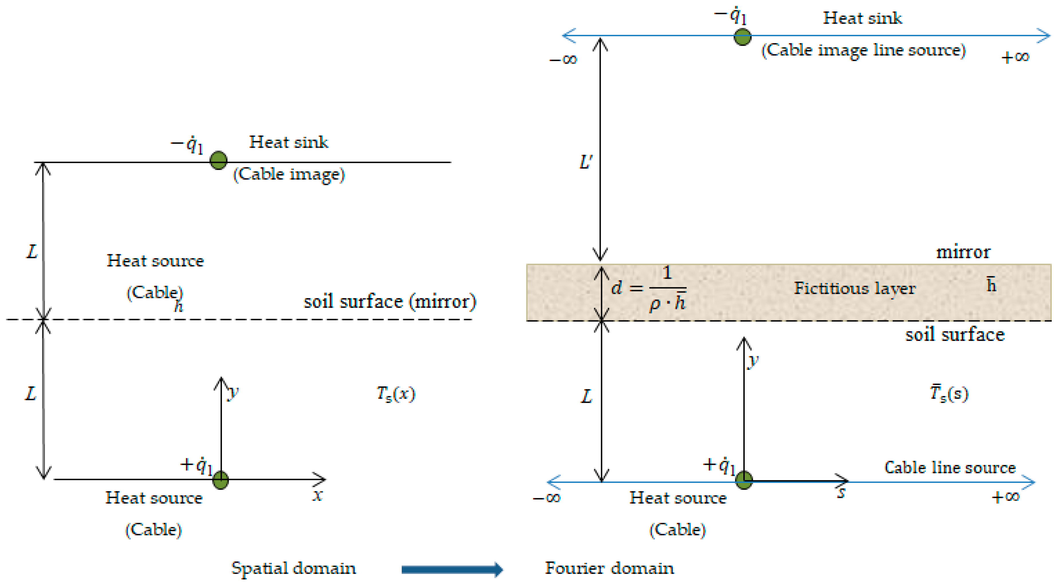
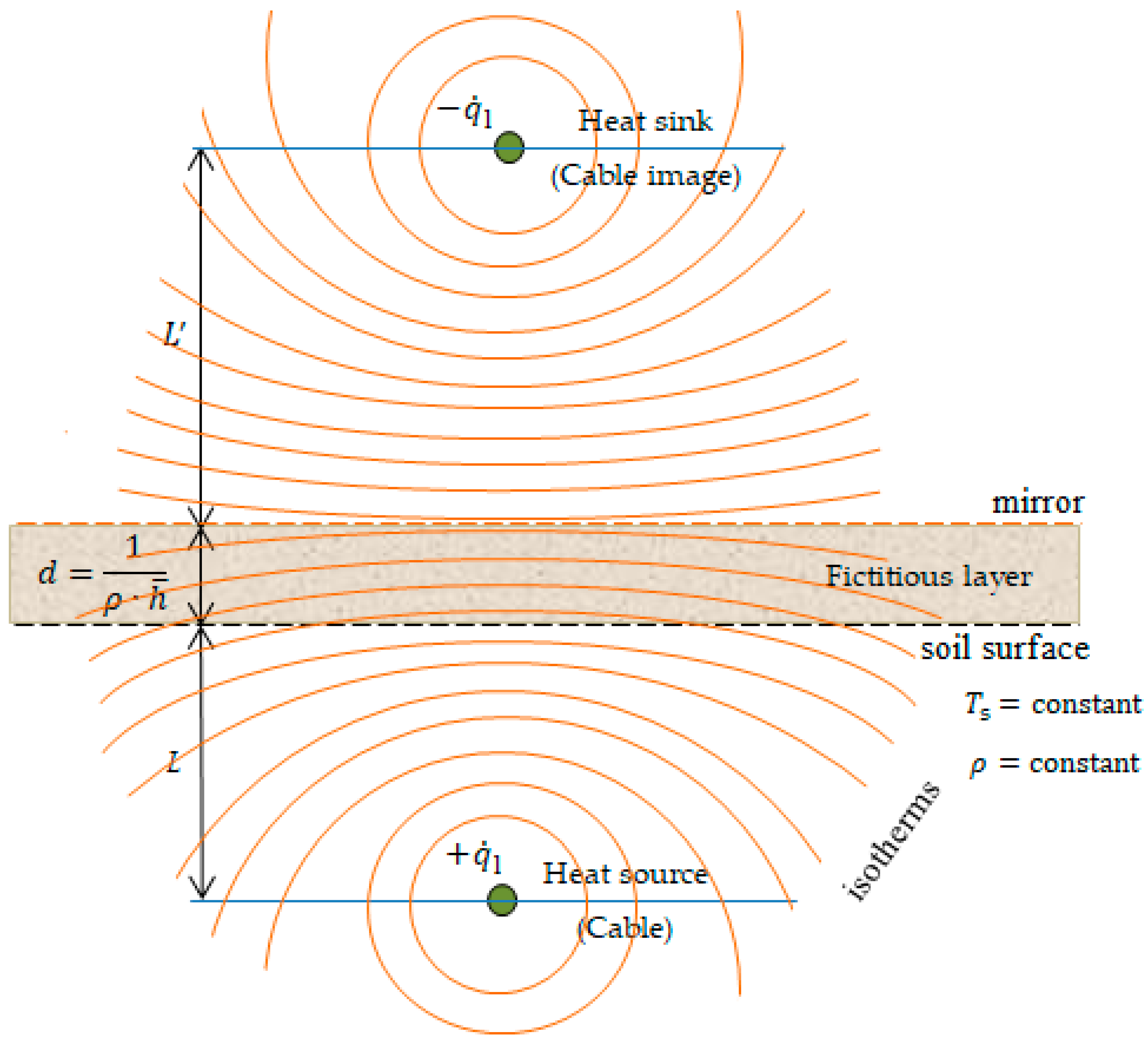
2.2. Non-Infinite Dimension of the Soil

In Equations (4) and (5), the soil is considered homogeneous and infinite. In this case, with a single cable, the thermal field is composed of concentric lines. In practice, the cables are buried at a given depth, and the shape of the thermal field depends on the presence of the ground surface. In turn, the ground surface can be considered at the same temperature or different temperatures. The traditional solution considers Kennelly’s hypothesis of having an isothermal interface between soil and air [18], further discussed in [19,20]. Kennelly’s hypothesis leads to the definition of the image method, which is useful to calculate the temperature growth at any point of the soil. The cable system is considered an infinitely long cylindrical heat source buried in a uniform medium, and it is not possible to consider the convective boundary conditions at the soil surface [9,21]. The heat source $+{\dot{q}}_{\mathrm{l}}$ (with thermal flux ${\dot{q}}_{\mathrm{l}}$ in W/m) is buried at a given depth in uniform soil. Heat is transferred from the heat source to all points having lower temperature by conduction. If the heat source is enclosed in a duct or pipe containing air, then the heat is also transferred by convection. The soil surface is considered as the symmetry axis. The heat sink, emitting the heat $-{\dot{q}}_{\mathrm{l}},$ is the reflected image of the heat source. The heat sink has the same distance L and magnitude above the soil surface as the heat source has below the soil surface. In the case of multiple cables, or cables with multiple cores in which the electric current flows, the superposition effect is applied [10].

The heat conduction equation due to the heat sink is:

$$\frac{\mathrm{d}T}{\mathrm{d}r} - \frac{\rho ·{\dot{q}}_{\mathrm{l}}}{2·\pi ·r} = 0 \Rightarrow \mathrm{d}{T}_{ \sin \mathrm{k}} = \frac{\rho ·{\dot{q}}_{\mathrm{l}}}{2·\pi }·\frac{\mathrm{d}r}{r} \Rightarrow T_{ \sin \mathrm{k}} = {{\displaystyle \int }}_{\infty }^{r^{\prime }}\frac{\rho ·{\dot{q}}_{\mathrm{l}}}{2·\pi }·\frac{\mathrm{d}r}{r}.$$

(7)

The heat conduction equation due to the heat source is:

$$\frac{\mathrm{d}T}{\mathrm{d}r} + \frac{\rho ·{\dot{q}}_{\mathrm{l}}}{2·\pi ·r} = 0 \Rightarrow \mathrm{d}{T}_{\mathrm{source}} = -\frac{\rho ·{\dot{q}}_{\mathrm{l}}}{2·\pi }·\frac{\mathrm{d}r}{r} \Rightarrow T_{ \mathrm{source}} = -{{\displaystyle \int }}_{\infty }^{r^{″}}\frac{\rho ·{\dot{q}}_{\mathrm{l}}}{2·\pi }·\frac{\mathrm{d}r}{r}.$$

(8)

The temperature increase at any point in the soil (in Figure 1, the point indicated is N) is the sum of two temperature increments (i.e., the temperature increment due to the heat source in the ground, and the temperature increment due to its fictive image above the soil):

$$\Delta T_{\mathrm{N}} = -{{\displaystyle \int }}_{\infty }^{r^{″}} \frac{\rho ·{\dot{q}}_{\mathrm{l}}}{2·\pi }·\frac{\mathrm{d}r}{r} + {{\displaystyle \int }}_{\infty }^{r^{\prime }}\frac{\rho ·{\dot{q}}_{\mathrm{l}}}{2·\pi }·\frac{\mathrm{d}r}{r} = \frac{\rho ·{\dot{q}}_{\mathrm{l}}}{2·\pi }\ln \frac{r^{\prime }}{r^{″}} \Rightarrow {\dot{q}}_{\mathrm{l}} = \frac{\Delta T_{\mathrm{N}}}{\frac{\rho }{2\pi }·\ln \frac{r^{\prime }}{r^{″}}} .$$

(9)

Consider the hypothesis that the outside diameter $D$ of the cable is much lower than the distance $L$ from the surface of the ground to the cable centre. Therefore, the temperature growth at the outside cable surface is [10]:

$$T_{\mathrm{line} \mathrm{source}}\left(\tau \right) \cong \frac{\rho ·{\dot{q}}_{\mathrm{l}}}{4·\pi }·\left[-\mathrm{Ei}\left(-\frac{D^2}{16·a·\tau }\right) + \mathrm{Ei}\left(-\frac{L^2}{a·\tau }\right)\right].$$

(10)

The effect of a non-isothermal ground surface is considered in [21] by adding a fictitious layer that moves the isothermal surface in the direction opposite to the cable location, as an application of the additional wall method shown in [22]. The adaptation proposed in the paper is based on applying the Fourier transform for converting the heat transfer problem from two dimensions to one dimension. In the transformed Fourier domain, the heat transfer coefficient is no longer dependent on soil thermal resistivity, installation depth, and cable dimensions; it depends only on the physical properties of the air and the heat that is dissipated by the cable. To model the non-isothermal soil surface, [21] proposed an accurate method in which the heat transfer coefficient may be computed in the Fourier domain. The application of this procedure was possible because, after the transformation in the Fourier domain, the heat transfer coefficient depends only on the air physical properties and the heat dissipated by the cable, and does not depend on cable dimensions, cable depth, and soil thermal resistivity $\rho$. This method has been shown to be compatible with standardized methods (IEC and IEEE).

The equation that describes the conversion of the two-dimensional heat transfer problem into a one-dimensional problem is:

$$F\left\{T\left(x,y\right)\right\} = \overline{T}\left(s,y\right),$$

(11)

where x and y, respectively, are the horizontal and vertical coordinates, $F\{.\}$ denotes the Fourier transformation, and s is the variable of the transformed Fourier domain.

Furthermore, the cable (the heat source) is defined as a Dirac function f(x) that is applied at a depth L with respect to the soil surface, in which ${\dot{q}}_{\mathrm{gen}}$ only appears at the position of the directly buried cable, and ${\dot{q}}_{\mathrm{l}} = 0$ anywhere else. In this case, the expression $F\left\{T\left(x,y\right)\right\} = 1$ points out that a buried cable in the space domain is expressed in the Fourier domain by a straight line with ${\dot{q}}_{\mathrm{l}} = \mathrm{constant}$(Figure 2). In the spatial domain, the soil temperature depends on the coordinate x, with the maximum temperature $T_{\mathrm{s}}$ at x = 0 (i.e., above the cable), progressively reduced when the coordinate x increases. In the Fourier domain, the cable is considered a constant line source, and the soil surface temperature ${\overline{T}}_s$ is constant. This temperature is iteratively calculated to verify the heat equation at the soil surface:

$${\overline{T}}_s = T_{\infty } + \frac{ {\dot{q}}_{\mathrm{l}}}{\overline{h}},$$

(12)

where $\overline{h}$ is the heat transfer coefficient in the Fourier domain.

The heat conduction equation (Laplace equation in steady-state, without ${\dot{q}}_{\mathrm{gen}}$) after the Fourier transformation is:

$$\frac{{\mathrm{d}}^2}{\mathrm{d}{y}^2}{\overline{T}}_s\left(s,y\right) = 0.$$

(13)

This equation satisfies the following boundary conditions:

$$\mathrm{at} y = L \Rightarrow \underset{{\dot{q}}_{\mathrm{conductive}}}{\underbrace{-k·\frac{\mathrm{d}{\overline{T}}_s\left(s,y\right)}{\mathrm{d}y}}} = \underset{{\dot{q}}_{\mathrm{convective}}}{\underbrace{\overline{h}·{\overline{T}}_s\left(s,y\right)}},$$

(14)

$$\mathrm{at} y = 0 \Rightarrow -k·\frac{\mathrm{d}{\overline{T}}_s\left(s,y\right)}{\mathrm{d}y} = {\dot{q}}_{\mathrm{l}}.$$

(15)

The solution of Equation (13) satisfying the boundary conditions (14) and (15) is:

$$\overline{T}\left(s,y\right) = -{\dot{q}}_{\mathrm{l}}·\rho ·y + \frac{{\dot{q}}_{\mathrm{l}}}{\overline{h}}·\left(1 + \rho ·L·\overline{h}\right).$$

(16)

The non-isothermal soil surface is modelled by introducing a fictitious layer with thickness d. The image of the cable line is then found at a distance $L^{\prime } = L + d$ (Figure 2).

In this case, the heat conduction equation after the Fourier transform is Equation (13).

Consider, the same line source. The boundary conditions are Equation (15) and the following equation:

$$\mathrm{at} y = L^{\prime } \Rightarrow -k·\frac{\mathrm{d}{\overline{T}}_s\left(s,y\right)}{\mathrm{d}y} = -{\dot{q}}_{\mathrm{l}}.$$

(17)

The temperature gradient is constant at y =$L^{\prime }$:

$$\overline{T}\left(s,y\right) = 0 .$$

(18)

The solution of the equation with these boundary conditions is:

$$\overline{T}\left(s,y\right) = -{\dot{q}}_{\mathrm{l}}·\rho ·y + {\dot{q}}_{\mathrm{l}}·\rho ·L^{\prime }.$$

(19)

By comparing Equation (16) with Equation (19), the thickness of the fictitious layer becomes:

$$d = \frac{1}{\rho ·\overline{h}}.$$

(20)

Figure 3 shows the scenario of when the fictitious layer is added. The mirror line is coincident with the horizontal isothermal line. In addition, different temperatures are found at the soil surface, which is crossed by other isothermal lines.

2.3. The Effect of the Ambient on the Soil Properties

Underground cables are buried at a given depth in the soil. The cable temperature can be affected by the phenomena occurring in the ambient, depending on the depth and on the presence of layers that reduce the effect of the external ambient, such as pavements or conduits. When the latter elements are absent, the variation of the temperature on the soil surface affects the internal part of the soil and the cable temperature. The effects can be seen on different time horizons.

In uniform soils, the heat flow is conductive. However, as indicated in [23,24], this assumption is not generally valid if there is a strong moisture gradient. The moisture gradient determines an isothermal vapour flux. In this case, part of the total soil evaporation results from subsurface evaporation that occurs under the soil surface. This evaporation affects the heat flux and the temperature profile.

The total soil heat flux ${\dot{q}}_{\mathrm{tot}}$ is given by the following equation:

$${\dot{q}}_{\mathrm{tot}} = {\dot{q}}_{\mathrm{latp}} + {\dot{q}}_{\mathrm{ds}},$$

(21)

where the isothermal latent heat flux ${\dot{q}}_{\mathrm{latp}}$ depends on the presence of a moisture gradient, and represents the latent heat carried from evaporating subsurface layers by the isothermal vapour flux [24], while ${\dot{q}}_{\mathrm{ds}}$ is the conductive soil heat flux, which incorporates only the thermal latent heat flux, and considering the soil depth $z$ is given by:

$${\dot{q}}_{\mathrm{ds}} = -k\frac{\mathrm{d}T}{\mathrm{d}z}.$$

(22)

During daytime, when a drying soil is heated, the thermal flux ${\dot{q}}_{\mathrm{ds}}$ is positive, while the thermal flux ${\dot{q}}_{\mathrm{latp}}$ is negative, and reduces the sum ${\dot{q}}_{\mathrm{tot}}$ at the soil surface. The variation of ${\dot{q}}_{\mathrm{ds}} \left(z,\tau \right)$ with the soil depth, depends on both temperature changes and the subsurface phase change (evaporation or condensation at the soil depth). The variation of ${\dot{q}}_{\mathrm{ds}} \left(z,\tau \right)$ leads to changes in the sensible and latent heats, to satisfy the energy conservation law:

$${\mathrm{C}}_{\mathrm{v}}·\frac{\partial \mathrm{T}}{\partial \mathsf{\tau }} = -\frac{\partial {\dot{q}}_{\mathrm{ds}}}{\partial \mathrm{z}} + {\dot{q}}_{\mathrm{gen}}\left(z,\tau \right),$$

(23)

where ${\dot{q}}_{\mathrm{gen}}$ is the rate of heat generated per unit volume for the local heat sink or source (e.g., water phase changes) in $\left[\frac{\mathrm{W}}{{\mathrm{m}}^3}\right].$

Neglecting ${\dot{q}}_{\mathrm{gen}}$ and the spatial variations in k, Equations (22) and (23) give the uncoupled heat diffusion equation:

$$\frac{{\partial }^{2}T}{\partial z^2} = \frac{1}{a}·\frac{\partial T}{\partial \tau }.$$

(24)

In cylindrical coordinates, the uncoupled heat diffusion equation becomes:

$$\frac{{\partial }^2\mathrm{T}}{\partial {\mathrm{r}}^2} + \frac{1}{\mathrm{r}}·\frac{\partial \mathrm{T}}{\partial \mathrm{r}} = \frac{1}{a}·\frac{\partial \mathrm{T}}{\partial \mathsf{\tau }}.$$

(25)

If heat and vapour flows are strongly coupled in the soil, the total soil heat flux is:

$${\dot{q}}_{\mathrm{tot}} = {\dot{q}}_{\mathrm{latp}} + \underset{{\dot{q}}_{\mathrm{ds} }= -\frac{\mathrm{d}T}{\mathrm{d}z}}{\underbrace{{\dot{q}}_{\mathrm{c}} + {\dot{q}}_{\mathrm{vT}}}} = ,$$

(26)

where ${\dot{q}}_{\mathrm{c}}$ is the conductive heat flux, and ${\dot{q}}_{\mathrm{vT}}$ is the thermal latent heat flux (both thermal fluxes are proportional to $-\frac{\mathrm{d}T}{\mathrm{d}z}$ and can be combined as ${\dot{q}}_{\mathrm{ds}}$) [24]. The energy conservation law in this case becomes the coupled equation [25]:

$${\mathrm{C}}_{\mathrm{v}}·\frac{\partial \mathrm{T}}{\partial \mathsf{\tau }} = -\frac{\partial {\dot{q}}_{\mathrm{tot}}}{\partial \mathrm{z}}.$$

(27)

The solution of the coupled equation needs numerical methods to be addressed. In fact, in general cases, many aspects cannot be solved analytically. With numerical methods, the soil is partitioned into adjacent volumes separated by boundaries. In this context, it is possible to model some particular cases with non-uniform soils, irregular boundary conditions, multi-dimensional flows, and non-linear equations.

Analytical solutions are possible under appropriate simplifications. In particular, these simplifications refer to considering uniform soil (or knowing the analytic representation of the variation of the soil thermal properties with depth) and assuming that the thermal properties of the soil do not change with the temperature. Further requirements to set up analytical solutions include the analytic representation of the boundary conditions and the initial conditions. Under these simplifications, it is possible to find the analytical solutions of two types of variation in time [24]:

(a)

periodic variations, determined with the Fourier transform; and

(b)

non-periodic variations, determined with the Laplace transform.

For periodic variations, starting from a time series with N values (where N is an even number), it is possible to calculate a number of harmonics not higher than H = N/2. The soil surface temperature is then expressed as:

$$T_s\left(\tau \right) = {\overline{T}}_s + {{\displaystyle \sum }}_{h = 1}^H{A}_h·\sin \left(h·{\omega }_1·\tau + {\phi }_h\right),$$

(28)

where ${\omega }_1 = \frac{2·\pi }{p}$ is the fundamental angular frequency, calculated by considering a period of 24 h when the daily wave is considered, or a period of 12 months for the annual wave; ${\overline{T}}_s$ is the mean temperature at the soil surface; $A_h$ is the amplitude of the h-th harmonic; and ${\phi }_h$ is the phase angle of the h-th harmonic.

The results of the Fourier analysis are rigorously valid when the wave is repeated without changes in successive time intervals, namely, each day for the daily wave, or each year for the annual wave. In addition, if the soil thermal properties do not vary with the depth, and the temperatures at all depths are assumed to vary around the same ${\overline{T}}_s,$ the depth penetration of soil surface temperature $T\left(z, \tau \right)$ is the sum of the penetrations of each harmonic [26]:

$$T\left(z, \tau \right) = {\overline{T}}_{\mathrm{s}} + {{\displaystyle \sum }}_{h = 1}^H{A}_h·e^{-\frac{z·\sqrt{h}}{D_1}}·\sin \left(h·{\omega }_1·\tau + {\phi }_h-\frac{z·\sqrt{h}}{D_1}\right),$$

(29)

where $D_1 = \sqrt{\frac{2a}{{\omega }_1}}$ is the damping depth of the fundamental $\left(h = 1\right)$.

More generally, changes in ${\overline{T}}_{\mathrm{s}}$ with the soil depth can be addressed by studying the evolution of ${\overline{T}}_{\mathrm{s},z}$ for different depths z, separately with respect to the sinusoidal terms.

From Equation (29), the conductive soil heat flux becomes:

$${\dot{q}}_{\mathrm{ds}} = {{\displaystyle \sum }}_{h = 1}^H{A}_h·\left(k·C_{\mathrm{v}}·h·{\omega }_1\right)·e^{-\frac{z}{D_h}}·\sin \left(h·{\omega }_1·\tau + {\phi }_h - z·D_h{}^{-1} + \frac{\pi }{4}\right),$$

(30)

where $D_h = \frac{D_1}{\sqrt{h}}$.

For non-periodic variations, the Laplace transform of $T\left(z, \tau \right)$ is a function of $z$ and the Laplace parameter $s$ only [27]:

$$L\langle T\left(z, \tau \right)\rangle = {{\displaystyle \int }}_0^{\infty }T\left(z, \tau \right)·{\mathrm{e}}^{-s·\tau }\mathrm{d}\tau .$$

(31)

The Laplace transform of Equations (24) and (25) is the ordinary differential equation [27]:

$$a·\frac{{\mathrm{d}}^{2}L \langle T\left(z, \tau \right) \rangle }{\mathrm{d}{z}^2}-s·L \langle T\left(z, \tau \right) \rangle +T\left(z,0\right) = 0.$$

(32)

Considering the difference $T^{\prime }\left(z, \tau \right)$ between $T\left(z, \tau \right)$ and an initial isothermal value of the soil, the boundary condition is expressed as:

$$T^{\prime }\left(z, 0\right) = 0,$$

(33)

and for a semi-infinite soil a solution to Equation (31) is:

$$L \langle T^{\prime }\left(z, \tau \right) \rangle = B·{\mathrm{e}}^{-z·{\left(\frac{s}{a}\right)}^{\frac{1}{2}}},$$

(34)

where B is a constant, which is a function of s and depends on the boundary conditions used.

2.4. Non-Homogeneous Soil

A detailed analysis of the soil thermal properties is needed for the design and installation of underground cables and pipelines, to avoid premature damages. The main thermal property to assess the soil is its thermal resistivity. The main aspects that affect the thermal resistivity are the soil type, the geometrical layout of the soil components, and the moisture content. The composition of the soil includes different particles, which form aggregates of sand, silt, colloids, and pore spaces. In addition, water may be present in the soil into different extents [19].

The soil thermal resistivity under loading conditions is found in the range of 0.5 to 1.2 m·K/W [28]. This value could become higher because of the heat dissipated from the underground cables. The heat dissipation phenomenon provokes the soil instability, leading to thermal damage of the cable [29]. The soil thermal resistivity is affected by the soil temperature, soil porosity, and water-vapour transport. The corresponding parameters have to be modelled, to avoid errors in the temperature distribution compared with real conditions [30].

The standard IEC 60287 [31] indicates how the effective thermal resistivity and thermal resistance of the soil can be calculated. The ability of the soil to keep its thermal resistivity constant in the presence of a heat source is named thermal stability of the soil [32]. The soil moisture content has a significant effect on buried cables capacity and soil thermal resistivity. The major concern is that the heat transfer from the cable into the soil leads to a considerable moisture migration far from the buried cable in the case of unfavourable conditions. Furthermore, around the cable, a dry zone characterized by uniform high thermal resistivity could form. This phenomenon occurs because air, considered as a weak conductor, divides the solid particles of the soil. If the soil moisture content increases, the soil thermal resistivity decreases because water is a good conductor. In the dry zone, the thermal resistivity in the dry state is considered. The wet zone is characterized by a thermal resistivity in the saturated state [33]. As such, the dry soil has a thermal resistivity higher than the wet soil. If in the beginning, the soil thermal resistivity decreases quickly as the moisture content is raised after a while, the decrease rate comes to be lower [34].

Gouda et al. [35] specified that in the presence of the dry zone, the capacity of the buried cable is decreased by applying a derating factor that depends on the type of soil. Outside the dry zone, the soil thermal resistivity is also uniform but corresponds to the soil moisture content [9]. The dry zone provokes an increment of temperature in the cable sheath. This phenomenon leads to a deterioration of the cable insulation and an eventual formation of hot spots in the cable [36]. A practical assumption that can be considered for practical purposes is that the dry zone does not modify the profile of the isotherms compared with their profile when the soil was moist. Only the numerical values of some isotherms are changed [10]. When the temperature difference between the external surface of the cable and the ambient temperature exceeds a critical limit (which depends on temperature, type of soil, and moisture content), the drying of the soil forms a zone in which the thermal resistivity increases. The isotherm corresponding to the critical limit gives the boundary of the dry zone. In the dry zone, the uniform (high) thermal resistivity is assumed. Outside the dry zone, a uniform thermal resistivity is also considered. The only changes from the uniform conditions of the soil depend on the non-uniformity is caused by drying. The assumption considered is no longer valid in the presence of backfills with different characteristics from the uniform soil around the cable. The probability of the soil drying out increases when the direction of the cable is crossed by another heat source [10]. The moisture migration induced by thermal gradient changes the thermal environment and needs appropriate modelling of the temperature response of the cable [37].

Donazzi et al. [38] specified that some backfill materials such as sand, cement, silt, as well as water, can be used to improve the thermal conditions of the cables. For example, the dry zone phenomenon in the backfill, initiated at various temperatures and velocities, depends on the soil type and the quantity of mud [35]. Donazzi et al. [38] also highlighted the significance of the critical water content, supposing that this is independent of the environment temperature in practice (when the soil temperatures around buried cables are less than 80 °C). Groeneveld et al. [39] experimentally demonstrated the effect of temperature on the critical water content in the soil and specified that a higher temperature reduces the capacity of water-keeping of soil. The effect of ambient temperature and ambient saturation on the temperature of the cable conductor is addressed in [40] and [30]. Moreover, the critical temperature for the formation of the dry zone, and the ratio of the dry to wet thermal resistivity, depending on the soil components but not on the loading on the cable. An essential factor to obtain the time required for the dry zone formation is the heat flux [41]. Both the critical temperature and the ratio of the dry to wet thermal resistivity do not depend on the heat flux transferred from the buried cables to the soil [36]. The heat flux at the cable surface is useful to obtain the time required for soil to get [41]. Some mathematical models have been developed, assessing the dry zone phenomenon around the buried cable [42,43,44,45,46,47].

The hot spots formed in the buried cable can be mitigated by using some solutions such as:

−

the addition of a corrective backfill with low thermal resistivity;

−

the heat sources around the buried cables must be insulated;

−

the forced convection for the fluid around the buried cable;

−

an insulating fluid for the inner cooling of the cable;

−

installing in the hot spot zone a forced cooling system [48].

One of the most used solutions to avoid soil drying around the cable is based on water cooling [48,49]. The most adopted practice is to install, in parallel with the buried cables, the pipes in which the cooling water passes. In this case, the heat transfer modelling must take into account the soil parameters, depth of cable burial, location of the water pipes, and other factors varying along the cable route. This cooling method is not proper for the extruded insulation cables—except for the case in which a tight sheath for water is used. Tobin et al. [48] proposed a prototype of a chilled-water heat removal system, applied to underground urban distribution systems. The proposed system raised the possibility of carrying current with about 60% for 13 to 115 kV cables. More recently, Klimenta et al. [50] proposed a solution based on hydronic asphalt pavements. In the case in which the water cooling cannot be used to reduce the hot spots, Brakelmann et al. [47] propose gravitational water cooling as a solution.

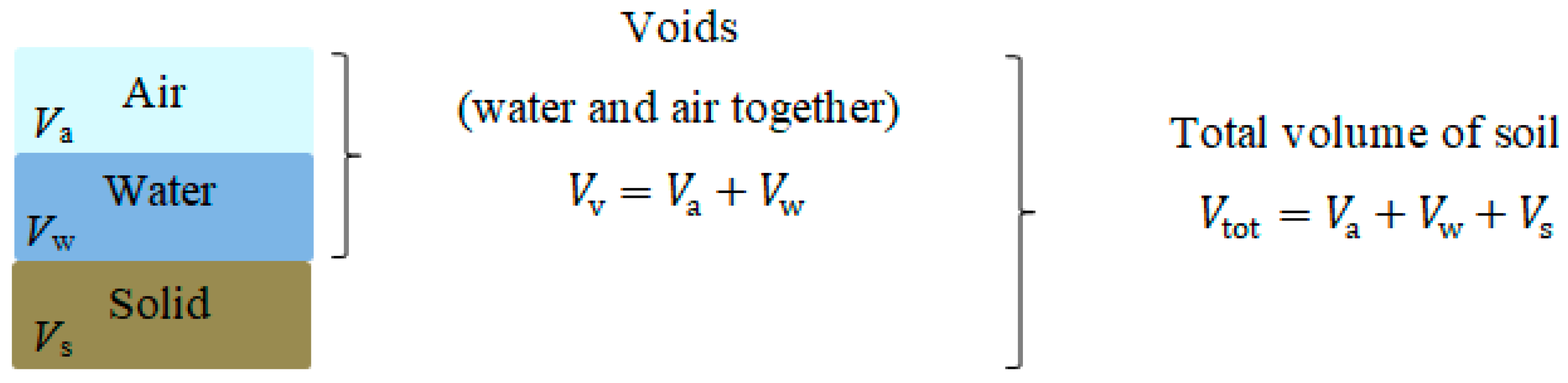
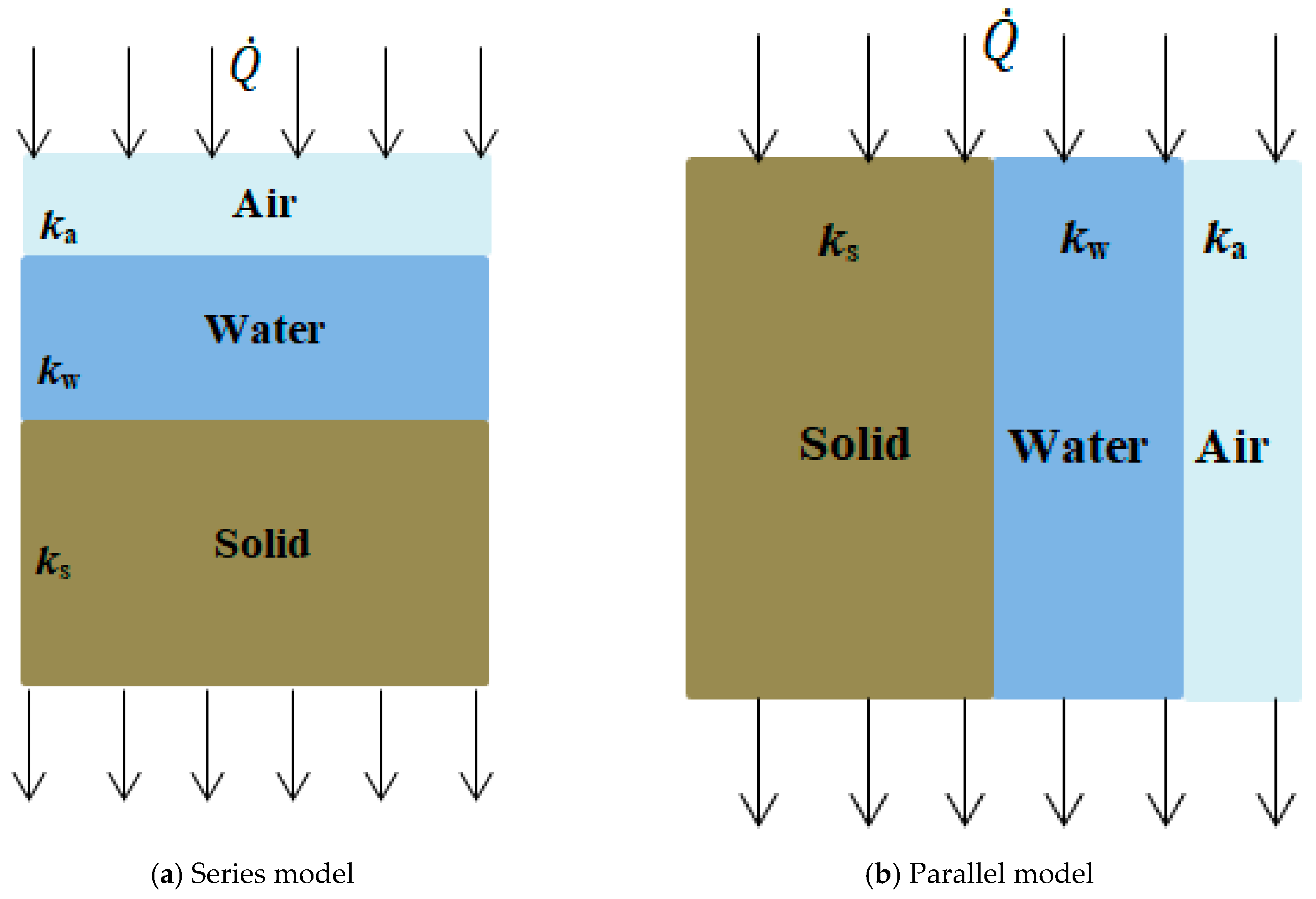
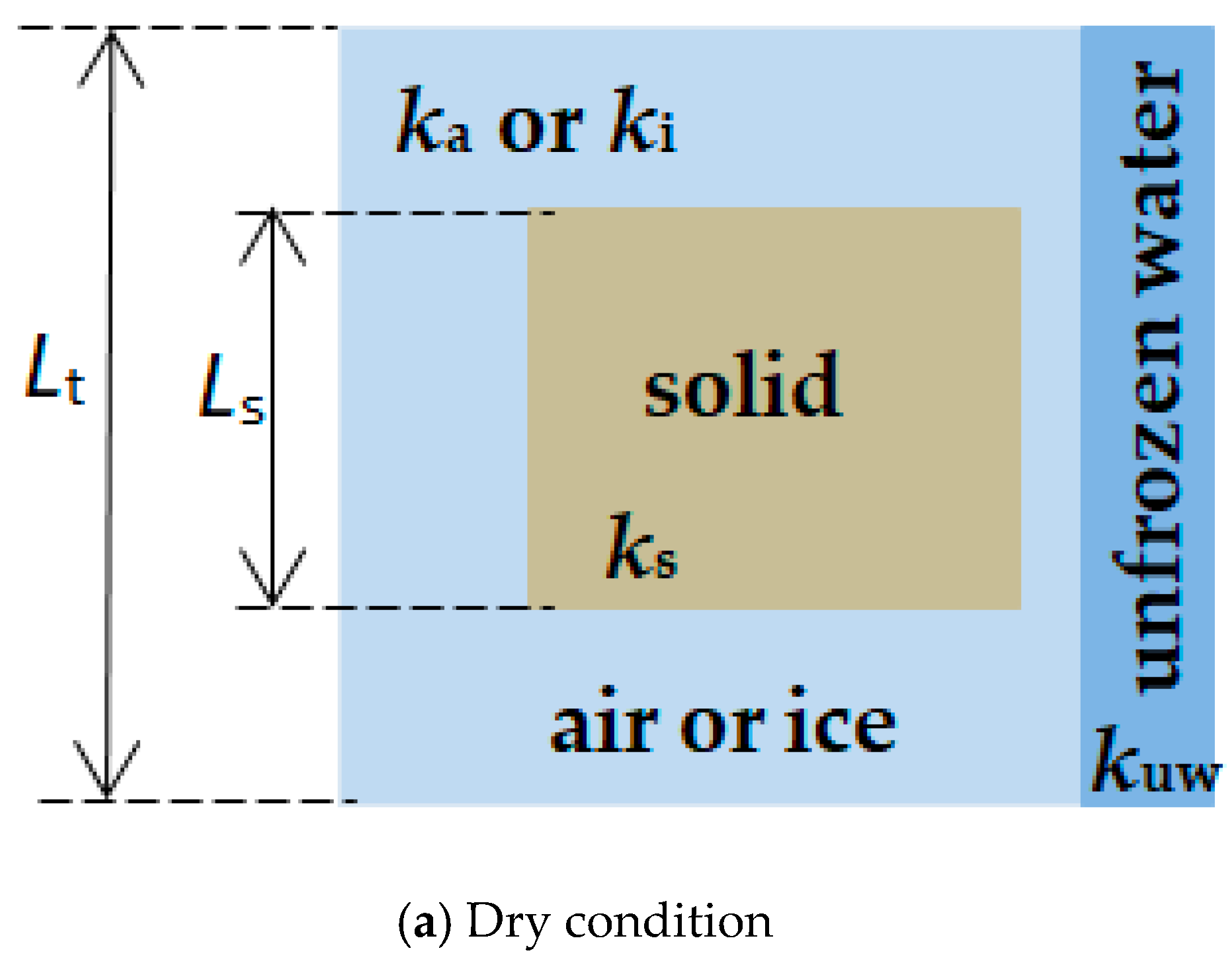
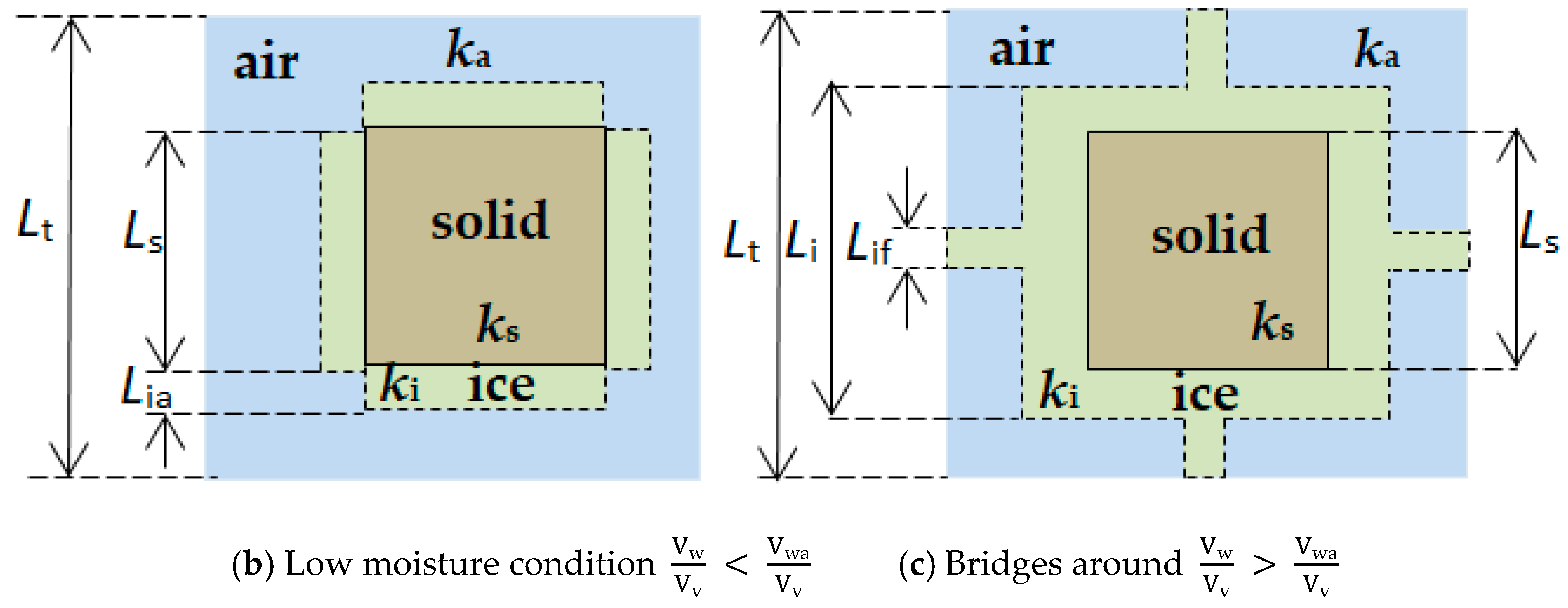
Effective Soil Thermal Conductivity

The effective thermal conductivity (k_eff) is a thermal property of a multi-phase (air, water, solid) soil. It represents the soil capacity to transfer heat by conduction under unit temperature gradient, as a function of the volumetric fractions of the soil microstructure, soil phases, and the phases connectivity [51,52].

The main factors that influence the effective thermal conductivity of soil under isothermal conditions are: soil mineralogy, solid particle shape and size, gradation, cementation, porosity, packing geometry, water content (or saturation degree), soil temperature, and stress level [53]. A synthesis of these factors is provided below.

In soil mineralogy, the soil is considered a multi-phase system (a three- or four-phase system) because its composition includes solid (mineral) particles, water, air, and sometimes ice (in some cold zones) [15]. The solid particles contain soil minerals (e.g., one of them is the quartz with the biggest thermal conductivity 8.4 W/(m$·$K) compared to other minerals, see [54]), which are surrounded by water and air [55].

Furthermore, the thermal conductivity of the dry soil at a temperature of 10 °C is less than 0.5 W/(m$·$K) and depends on the packing density and mineral composition [56]. In the dry zone, the air impedes heat conduction, and this heat transfer phenomenon takes place through the contact points of the solid particles. If air is replaced by water, a significant enhancement of the heat conduction is observed. Therefore, the order of the thermal conductivities is $k_{\mathrm{air}} < k_{\mathrm{dry} \mathrm{soil}} < k_{\mathrm{water}} < k_{ \mathrm{water}-\mathrm{saturated} \mathrm{soil}} < k_{\mathrm{mineral}}$ [15,56,57,58].

Solid particle size and shape have a significant influence on the positioning of primary and secondary solid particles. In natural soils, the soft particles are included into bigger particles of different sizes and shapes. In addition, the number of contact points of the solid particles has a significant influence on the soil thermal conductivity. As it is known, the heat transfer in soils relies on the solid phase and occurs across the contact points, especially in the dry zone, because the air thermal conductivity is reduced compared to the solid particles of soil (the air thermal conductivity is 0.0026 W/(m$·$K)) [16]. Moreover, fewer contact points and bigger solid particles lead to increased soil thermal conductivity [59].

Gradation represents the distribution of various sizes of individual solid particles inside a soil zone. The soil with a good gradation presents a good heat transfer because the little solid particles fill the interstitial space of pores and raise the coordinates among the solid particles [15].

Cementation also influences soil thermal conductivity if the solid particles of soil are cemented together by binders or clay (the thermal conductivity is 1.28 W/(m$·$K) [54] the contact area will increase. The soil thermal conductivity will majorly increase [60,61].

Porosity influences soil thermal conductivity. The void ratio is a parameter to assess the compactness soil and represents the ratio between the voids volume to the solid volume. Based on the sketch of the volumetric ratios of soils shown in Figure 4, the void ratio is calculated as follows:

$$e = \frac{V_{\mathrm{v}}}{V_{\mathrm{s}}} = \frac{\sigma }{1-\sigma }.$$

(35)

The lower the void ratio, the greater the thermal conductivity [57]. Porosity is the ratio between the voids volume and total or bulk volume of soil.

$$\sigma = \frac{V_{\mathrm{v}}}{V_{\mathrm{tot}}} = \frac{e}{1+e}.$$

(36)

Packing geometry highlights that good coordination among the solid particles increases the soil thermal conductivity [60]. The packing density is the ratio between the solid volume to the total volume,

$${\zeta }_{\mathrm{p}} = \frac{V_{\mathrm{s}}}{V_{\mathrm{tot}}}.$$

(37)

The effect of the soil density on soil thermal conductivity is relatively low. The rise of the soil density leads to the significant growth of the contact point’s number, but not at a substantial increment of the soil thermal conductivity [62].

Water content plays an important role in obtaining soil thermal conductivity. In unsaturated soils, the growth of the soil thermal conductivity with the water content increase highlights the significant contribution of the pore conduction [15,34]. Water movement also influences soil thermal conductivity. At temperatures less than 0 °C the water frozen in the soil and the soil thermal conductivity are modified. Conversely, at high temperatures, water is changed into water vapour molecules, and the soil thermal conductivity increases.

The influence of the soil temperature on the soil thermal conductivity is analysed in [63]. The thermal conductivity of nine soil samples at the soil temperature ranging from 30 to 90 °C was measured. The results showed that in moist soil, the thermal conductivity had a significant increment with the soil temperature, obtaining values three to five times the 30 °C value when the sample soil temperature was 90 °C. Hiraiwa and Kasubuchi [64] noted that in the case of sandy soils, the soil thermal conductivity increased as the temperature of the soil increased. Tarnawski and Gori [65] measured the thermal conductivity of the soil for soil temperatures ranging from 5 to 90 °C in the case of four soil moisture content domains. They demonstrated that soil thermal conductivity has a low variation with the soil temperature and water content at reduced moisture contents. Smits et al. [66] measured thermal conductivity for two grains of sand with different solid particle sizes for a temperature range from 30 to 70 °C and variable saturation. They observed that the increase of the soil thermal conductivity with the temperature is for temperatures higher than 50 °C at low to intermediate saturation. When the soil is close to saturation, and at the lowest saturations, the temperature did not have a measurable effect on the thermal conductivity. At the temperatures ranging from 30 to 50 °C, the thermal conductivity has a small variation with the temperature.

Stress level also plays an important role, in the sense that higher stress leads to higher contact radii resulting in an increment of the soil thermal conductivity. In addition, under higher stress, the granular chains enhance the heat transfer in soil [15,67]. Many thermal conductivity models have been proposed to obtain accurate predictions of the effective thermal conductivity. The models have been divided into three model types: mixing models, empirical models, and mathematical models.

The mixing models, called theoretical/physical models, consider the soil as a three-phase system (solid, water and air) in which the phases are represented as a particular combination of series and parallel in the soil sample [15]. The mixing models are based on the mixing laws (arithmetic, geometric, and harmonic mean) of the series model and parallel model. The series and parallel models refer to Wiener bounds (or upper and lower bounds) of thermal conductivity and do not depend on the pore structure of porous medium [68]. Combinations of such series and parallel models are extensively presented in [15].

The series model considers a constant heat flux through each layer (Figure 5a). The phases have different thermal conductivities and develop different temperature gradients [15].

In this case, the effective thermal conductivity of soil is:

$$\frac{1}{k_{\mathrm{eff}}} = {\left[{{\displaystyle \sum }}_{n = 1}^M{\mu }_n·\frac{1}{k_n}\right]}^{-1},$$

(38)

where $M$ is the number of phases (M = 3 for air, water, and solid), ${\mu }_n$ is the volume fraction of each phase, and $k_n$ is the thermal conductivity of each phase.

The parallel model considers a different heat flux through each phase that depends on the thermal conductivity of each phase (Figure 5b). The phases develop the same temperature gradients.

In this case, the effective thermal conductivity of soil is:

$$k_{\mathrm{eff}} = {{\displaystyle \sum }}_{n = 1}^M{\mu }_n·k_n.$$

(39)

Another theoretical model is the De Vries model [23] and its simplified form presented in [69]. The De Vries model considers the soil as a mixture of ellipsoidal particles aleatory placed in the wet soil (continuous water) or the dry soil (ambient). In the wet soil, the solids and air represent the dispersed phase (the phase that is present in the particle shape), and in the dry soil, the solids and water represent the dispersed phase. The De Vries model requires many shape factors of ellipsoidal particles that are difficult to obtain. In this case, the effective thermal conductivity is very influenced by the shape factors and water content [70].

The effective thermal conductivity is:

$$k_{\mathrm{eff}} = \frac{{{\displaystyle \sum }}_{i = 0}^{M-1}{G}_i·k_i·{\theta }_i}{{{\displaystyle \sum }}_{i = 0}^{M-1}{G}_i·{\theta }_i},$$

(40)

where $M$ is the number of phases (air, water, solid); $G_i$ is the percentage of the mean temperature gradient of each phase. It is influenced by the shape factors of the ellipsoidal particles and soil components. The case $i = 0$ represents the continuous phase, ${\theta }_i$ is the volume fraction of each phase; $G_i$ is the percentage of the mean temperature gradient along with each phase; and $k_i$ is the thermal conductivity of each phase.

The model developed by Gori [71] was based on a soil cubic mixing cell and consists of a comparison between the analytical predictions and the experimental results of the effective thermal conductivity. The hypothesis to obtain the effective thermal conductivity was to consider parallel and horizontal isotherms or vertical heat flux lines. The experimental data obtained in [71] on the unsaturated frozen soils showed that the hypothesis with parallel and horizontal isotherms better predicts the effective thermal conductivity.

In the case of saturated frozen or dry soils, a cubic cell representing the soil was placed inside a cubic space (Figure 6a). The unfrozen water was distributed along the cubic cell length $L_{\mathrm{t}}$. Furthermore, the ratio between the cubic cell length $L_{\mathrm{t}}$ and the solid length $L_{\mathrm{s}}$ depends on the soil porosity.

In the case of the parallel and horizontal isotherms, the analytical expression of the effective thermal conductivity is:

$$\frac{1}{k_{\mathrm{eff}}} = \frac{1 - \frac{L_{\mathrm{t}}}{L_{\mathrm{s}}}}{k_{\mathrm{c}}·\left(1 - u_{\mathrm{w}}\right) + k_{\mathrm{w}}·u_{\mathrm{w}}} + \frac{\frac{L_{\mathrm{t}}}{L_{\mathrm{s}}}}{k_{\mathrm{c}}·\left[{\left(\frac{L_{\mathrm{t}}}{L_{\mathrm{s}}}\right)}^2·\left(1 - u_{\mathrm{w}}\right) - 1\right] + k_{\mathrm{w}}·u_{\mathrm{w}}·{\left(\frac{L_{\mathrm{t}}}{L_{\mathrm{s}}}\right)}^2 + k_{\mathrm{s}}},$$

(41)

where $k_{\mathrm{eff}}$ is the effective thermal conductivity for parallel and horizontals isotherms, ${\rho }_{\mathrm{T}} = \frac{1}{k_{\mathrm{T}}}$ is the effective thermal resistivity, and $k_{\mathrm{c}}$ is the thermal conductivity of continuous phase (for the frozen soils $k_{\mathrm{cp}} = k_{\mathrm{i}}$ and for the dry soils $k_{\mathrm{cp}} = k_{\mathrm{a}})$. The other thermal conductivities refer to the ice ($k_{\mathrm{i}}$), the air ($k_{\mathrm{a}}$), the water ($k_{\mathrm{w}}$), and the solid ($k_{\mathrm{s}}$). Furthermore, $u_{\mathrm{w}} = \frac{V_{\mathrm{uw}}}{V_{\mathrm{tot} \mathrm{cell}}}$ is the ratio between the unfrozen water volume and the total volume of the cubic cell, $V_{\mathrm{uw}}$ is the unfrozen water volume, $V_{\mathrm{tot} \mathrm{cell}}$ is the cubic cell volume.

In the case of the unsaturated frozen soils, the analytical expressions of the effective thermal conductivity are more complex and are computed for two cases: the water content is less than the ratio $\frac{{\mathrm{V}}_{\mathrm{wa}}}{{\mathrm{V}}_{\mathrm{v}}}$ (Figure 6a); the water content is higher than the ratio $\frac{{\mathrm{V}}_{\mathrm{wa}}}{{\mathrm{V}}_{\mathrm{v}}}$ (Figure 6b).

In the Gori model, the solid phase is placed in the centre, with the bridges increasing around the solid particle or water films. The remaining space is occupied with the air. The change of solid, water and air in the dry condition, low moisture condition and unsaturated condition with bridges around is shown in Figure 6.

Other theoretical models are widely presented in [16] and [51]. The theoretical models depend on a number of correlated factors, such as the ones recalled at the beginning of this subsection. Hence, the formulation of these models is quite challenging [52].

The empirical models are based on the mathematical and numerical assessment of experimental values between effective thermal conductivity and the measured soil properties (such as the degree of saturation or temperatures) [51]. The empirical models determine the expression between the relative thermal conductivity and the water content or saturation degree by normalizing the effective thermal conductivity [72]. The normalized thermal conductivity affirms that the effective thermal conductivity is estimated with the Kersten number, that is a linear combination of the saturated thermal conductivity $k_{\mathrm{sat}}$ and the dry soil conductivity $k_{\mathrm{dry}}$ [73]:

$$K_{\mathrm{e}} = \frac{k_{\mathrm{eff}} - k_{\mathrm{dry}}}{k_{\mathrm{sat}} - k_{\mathrm{dry}}} \Rightarrow k_{\mathrm{eff}} = K_{\mathrm{e}}·\left(k_{\mathrm{sat}} - k_{\mathrm{dry}}\right) + k_{\mathrm{dry}}.$$

(42)

The saturated thermal conductivity $k_{\mathrm{sat}}$ is determined with the geometric mean method:

$$k_{\mathrm{sat}} = k_{\mathrm{w}}^{\sigma }·k_{\mathrm{s}}^{1-\sigma },$$

(43)

where $\sigma$ is the porosity.

The dry thermal conductivity $k_{\mathrm{dry}}$ can be expressed in function of the porosity [73]:

$$k_{\mathrm{dry}} = \frac{\sigma + 6.65·\left(1 - \sigma \right)}{\sigma + 0.053·\left(1 - \sigma \right) } \pm 20\%,$$

(44)

The upper bound and the lower bound that appear in Equation (44) are not considered for the sake of facilitating the calculation. New empirical models have been formulated by various researchers by modifying this model [16,51,52].

The mathematical models are adapted from predictive models of physical properties. These properties are electric and hydraulic conductivities, dielectric permittivity, and magnetic permeability. These models are calculated by using the mathematical methods that take into account the volume fractions and thermal conductivity of each phase [51]. The details about these models are extensively presented in [16,51].

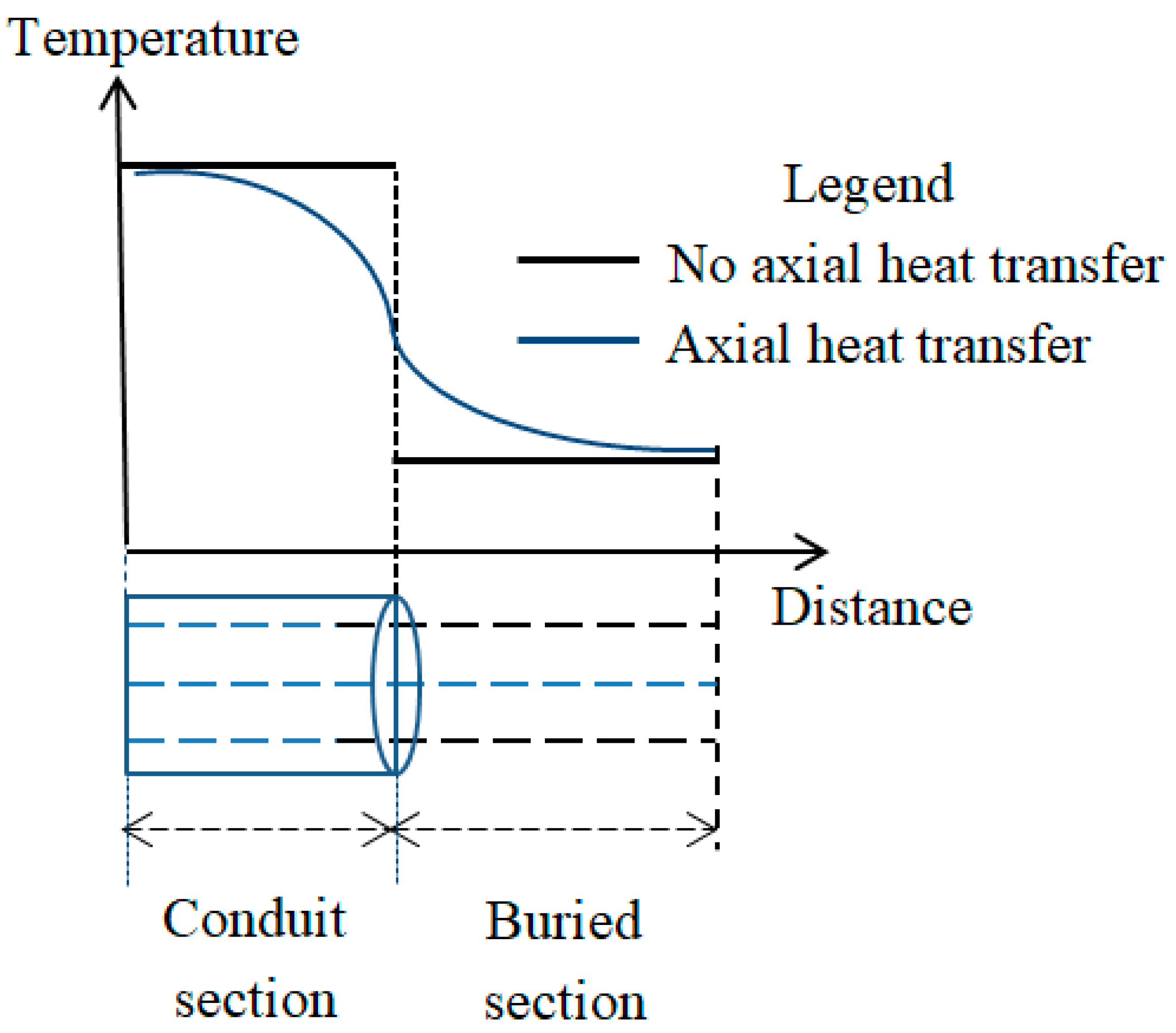
2.5. Finite Cable Length

The general hypothesis for carrying out studies of cable rating is that the cable length is virtually infinite. However, in some cases, there are situations in which this hypothesis is no longer true. An example is the short-conduit, typically used for providing additional protection to buried cables that cross the streets or pass near other pipelines [74]. The length of the short-conduit and the conditions of heat dissipation depend on the specific case. The short-conduit cable is composed of a buried section and a conduit section (Figure 7). The classical methods, as well as the method indicated in the standard IEC 60287 [75], cannot be applied directly to this situation. An approximation is possible only if the heat transfer along the axis is not modelled. However, in actual conditions, the heat dissipation is better in the buried section. Hence, part of the heat generated in the conduit section reaches the buried section in the axial direction, creating an axial temperature gradient [73]. For this reason, the calculations carried out by ignoring the axial phenomena lead to incorrect results for the assessment of the thermal cable phenomena, with possible underestimation of the maximum temperature in the buried section and overestimation of the maximum temperature in the conduit section. The latter would create a disadvantage for the full usage of conduit sections [73].

The effects of the length of the short-conduit cable, buried depth and soil resistivity have been investigated in [76] through 3D thermal simulations. In general, the initial point for the computation of the cable radial temperature has been based on a known thermal parameter of the environment [77,78]. In practice, however, the soil thermal conductivity is variable. For short-conduit cables, the accurate determination of the thermal environmental parameters in real-time is a challenging task. For this purpose, a specific method for determining the current real-time capacity of short-conduit cables has been proposed in [73]. A simplified quasi-3D thermal model is set up, and an iterative procedure is formulated starting from the real-time temperature at the conduit surface, measured in the conduit section, the temperature at the cable surface in the buried part, as well as the current that flows in the cable. The axial heat flow is updated during the iterations, together with the other variables.

2.6. Lack of Geometrical Symmetry

Even when the cable is modelled as a system with cylindrical symmetry (also including possible junctions), the overall system around the cable could not be geometrically symmetric. For example, for cables in conduits, a simple geometrically symmetric structure could adopt a concentric configuration. However, this configuration is not physical and does not correspond to the symmetric distribution of the temperatures, mainly because of convection. In [79], physical non-symmetric cases with “eccentric” and “cradle” configurations have been analysed, indicating that one of the main shortcomings in setting up a thermal model could be the over-simplification of the cable location in unfilled conduits. The effect is that the average temperature at the conductor-insulation interface in the case of concentric formation can be higher than for the eccentric and cradle configurations.

Other causes of lack of symmetry appear in helicoidal cables [80], in which the location of the cores changes at different horizontal cross-sections. Modelling such a system requires a software tool able to support 3D simulations, and the preparation of the geometry would be better supported by the definition of the symmetric structure, followed by the application of a torsional operator.

Non-symmetry also appears when a failure occurs in a given point of the cable. In this case, the properties of the materials change around the failure point and can create more non-symmetry when the failure evolves in time. This thing makes the cable modelling in transient conditions more complex, but is also relevant to the identification of failure paths, leading to hot spots and progressive deterioration of the materials. In this case, lack of symmetry also appears when there are multiple cables close to each other and the effect of the cable failure during time causes thermal effects to other cables, with temperature variations due to the mutual thermal coupling.

2.7. Non-Buried Cables

The underground cables mainly addressed in this paper cover most of the existing installations. However, there are other installations for which the thermal model has to be adapted. Some cases are described in chapter 10 of [9], including cables located within protective walls (such as covered trays, protective risers, or tunnels), and cables placed in uncovered trays. When the cables are installed in air, the main heat transfer mode becomes the convection, either natural, or forced (if an airflow along the cable is present), and radiation. In contrast, conduction in the air is typically neglected [9].

Submarine cables are used in high voltage direct current electric transmission systems, generally with single-core cables. For submarine cables, in any case, part of the path close to the cable terminals is buried in the soil, and is typically the bottleneck on the thermal side, with the possible occurrence of high temperatures. Among the various solutions, using a cooling pipe with circulating water would improve the thermal conditions [81]. In this case, the thermal model becomes more elaborated, to include the effects of the solutions for cooling the cable.

In recent years, with the progressive integration of offshore wind farms, the number of three-core submarine cables has increased. For these cables, specific thermal analysis is needed, taking into account the internal and external characteristics. Submarine cables are subject to thermo-mechanical stresses, which can be analysed in a multi-physics environment [82]. Further issues that appeared, owing to the increased usage of submarine cables for offshore applications, include the crossings among submarine cables, which can cause temperature increase at the crossing points. These cases cannot be handled by using the classical image method, and their analytical formulation would also depend on the model of the subsea thermal environment [83]. In particular, in this thermal environment, the effect of sediments on the heat transfer characteristics is not negligible [84]. The sediments are a mixture of solid and liquid components, which impact on conductive heat transfer. Moreover, if the permeability of the sediments is high, the convective heat transfer can be significant [85]. The thermal properties of the sediments (e.g., thermal conductivity and volumetric heat capacity) have to be considered in the overall thermal model.

3. Thermal Models and Thermal Analysis Methods

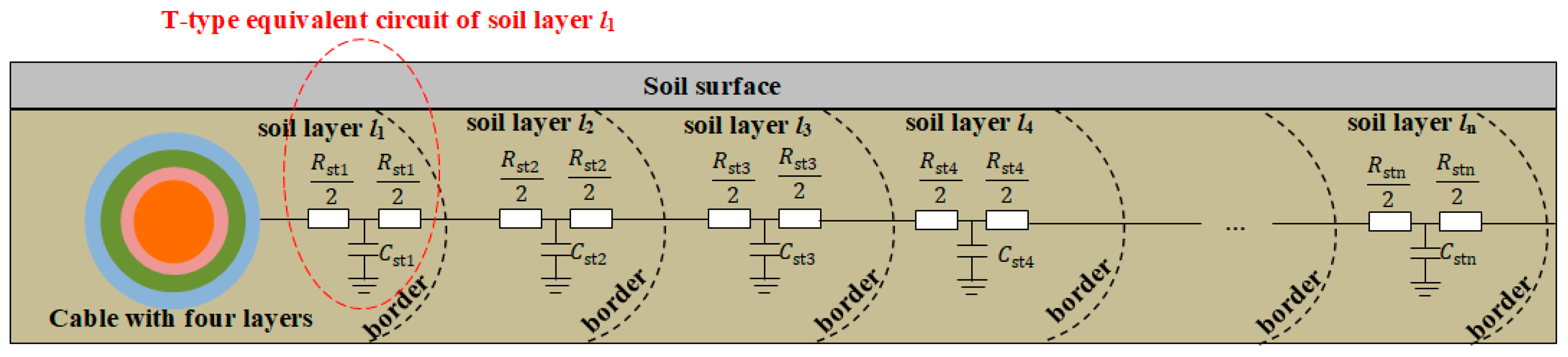
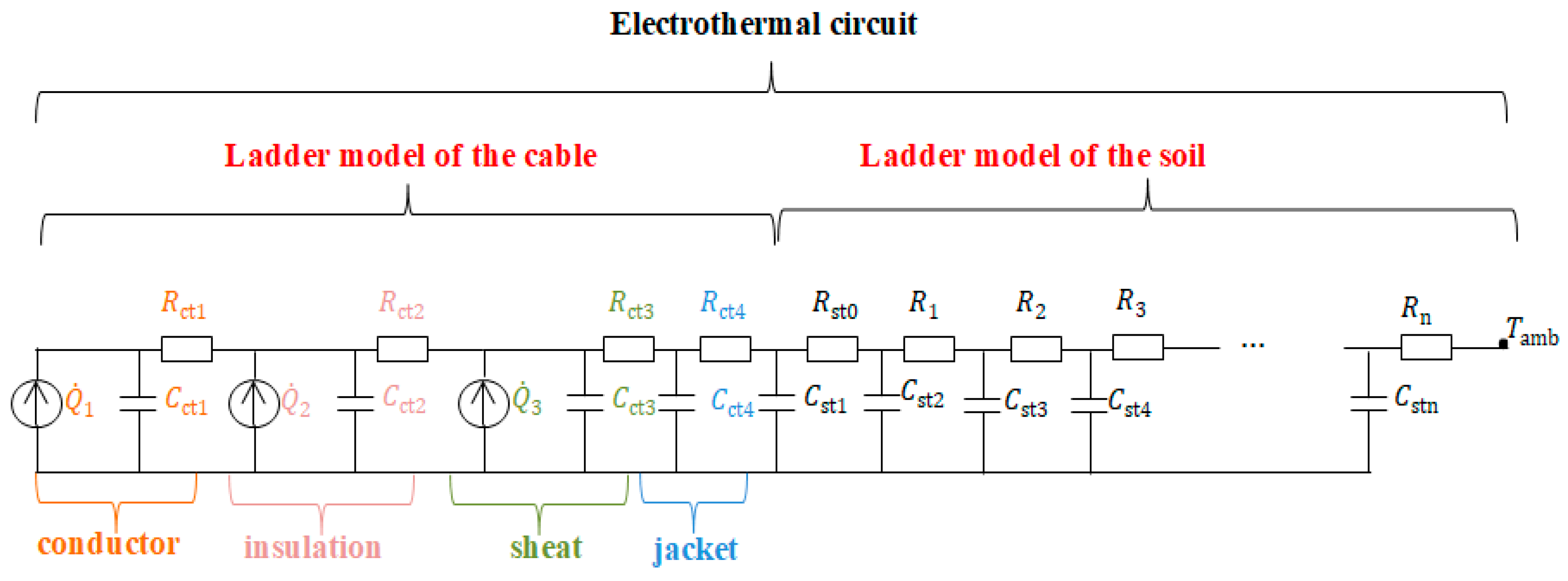
3.1. Thermal Models of Power Cables and Electrothermal Analogy

The thermal resistance R_t is the ratio of the temperature difference between the two faces of a material to the rate of heat flow per unit area. The thermal capacitance C_t represents the ability of a material to absorb and store the heat for using it later. In the electrothermal analogy, the thermal circuit is modelled by representing an equivalent electrical circuit, in which currents are equivalent to heat flows, and voltages are equivalent to temperatures. If the thermal parameters are independent of temperature, the equivalent circuit is linear. In this case, to solve a heat transfer problem, the superposition principle is applied [10].

The conductive thermal resistance of a cylindrical wall (e.g., cable insulation) having the inner diameter $d_{\mathrm{i}}$ and the outer diameter $d_{\mathrm{e}}$ is:

$$R_{\mathrm{t} \mathrm{cond}} = \frac{\rho }{2\mathsf{\pi }}\ln \frac{d_{\mathrm{e}}}{d_{\mathrm{i}}},$$

(45)

where $\rho$ is the thermal resistivity.

The conductive thermal resistance of a plane wall is:

$$R_{\mathrm{t} \mathrm{cond}} = \rho \frac{\delta }{S_{\mathrm{cond}}},$$

(46)

where $\delta$ is the thickness of the wall, and $S_{\mathrm{cond}}$ is the cross-section of the wall.

The convective thermal resistance is:

$$R_{\mathrm{t} \mathrm{conv}} = \frac{1}{h_{\mathrm{conv}}·S_{\mathrm{conv}}},$$

(47)

where $S_{\mathrm{conv}}$ is the convective heat transfer surface, and $h_{\mathrm{conv}}$ is the convective heat transfer coefficient.

The radiative thermal resistance is:

$$R_{\mathrm{t} \mathrm{rad}} = \frac{1}{h_{\mathrm{rad}}·S_{\mathrm{rad}}},$$

(48)

where $S_{\mathrm{rad}}$ is the radiative heat transfer surface, and $h_{\mathrm{rad}}$ is the radiative heat transfer coefficient.

The total heat transfer coefficient for a cable installed in air is:

$$h_{\mathrm{total}} = h_{\mathrm{conv}} + h_{\mathrm{rad}}.$$

(49)

The thermal capacity C_t for a coaxial configuration (e.g., cylindrical insulation of a cable) having the inner diameter $d_{\mathrm{i}}$ and the outer diameter $d_{\mathrm{e}}$, is:

$$C_{\mathrm{t}} = \underset{V}{\underbrace{\frac{\pi ·d}{4}·\left(d_{\mathrm{e}}{}^2 - d_{\mathrm{i}}{}^2\right)}}·c_{\mathrm{p}},$$

(50)

where V is the volume of the cylindrical configuration.

The thermal conductance is a measure of the rate of heat flow through a body, and it is the reciprocal of the thermal resistance:

$$K = \frac{1}{R_{\mathrm{t}}}.$$

(51)

The typical thermal models of the cables have been constructed by resorting to the electrothermal analogy (

Table 1. Electrothermal analogy.

Electrical Parameters	Symbol and Unit	Thermal Parameters	Symbol and Unit
Electric conductivity	$\nu \left[{\left(\mathsf{\Omega }·\mathrm{m}\right)}^{-1}\right]$	Thermal conductivity	$k \left[\mathrm{W}·{\left(\mathrm{m}·\mathrm{K}\right)}^{-1}\right]$
Electric resistance	$R_{\mathrm{e}} \left[\mathsf{\Omega }\right]$	Thermal resistance	$R_{\mathrm{t}}\left[\mathrm{m}·\mathrm{K}·{\mathrm{W}}^{-1}\right]$
Electric current	$I \left[\mathrm{A}\right]$	Heat flow rate	$\dot{Q} \left[\mathrm{W}\right]$
Capacitance	$C_{\mathrm{e}} \left[\mathrm{F}\right]$	Thermal capacity	$C_{\mathrm{t}}\left[\mathrm{J}·{\mathrm{K}}^{-1}\right]$
Electric potential	$U \left[\mathrm{V}\right]$	Absolute temperature	$T \left[\mathrm{K}\right]$
Ground potential	$0 \left[\mathrm{V}\right]$	Absolute zero	$0 \left[\mathrm{K}\right]$

). Mostly, the resistors represent the thermal resistances; the capacitors represent the thermal capacities, which are essential to model the thermal transients in real operating conditions. The generators represent the heat sources due to different types of losses (e.g., Joule losses in the conductor, dielectric losses, and losses in the sheath and armour) [11,86].

In

Table 2. Values of thermal resistivity and thermal capacity for some materials [10].

Material	Thermal Resistivity [(m·K)/W]	Thermal Capacity (c·10−6) [J/(m3·K)]
Insulating materials
Paper insulation in solid-type cables	6.0	2.0
Paper insulation in oil-filed cables	5.0	2.0
PE	3.5	2.0
XLPE	3.5	2.0
Polyvinyl chloride for up to and including 3 kV cables	5.0	1.7
Polyvinyl chloride for greater than 3 kV cables	6.0	1.7
EPR for up to and including 3 kV cables	3.5	2.0
EPR for greater than 3 kV cables	5.0	2.0
Protective coverings
Compounded jute and fibrous materials	6.0	2.0
Rubber sandwich protection	6.0	2.0
Polychlroprene	5.5	2.0
PVC for up to and including 35 kV cables	5.0	1.7
PVC for greater than 35 kV cables	6.0	1.7
PE	3.5	2.4
Materials for duct installations
Concrete	1.0	2.3
Fiber	4.8	2.0
Asbestos	2.0	2.0
Earthenware	1.2	1.8
PVC	3.5	2.4
PE	3.5	2.4

, the values of thermal resistivity and thermal capacity for some materials and soils in different conditions are reported. Typical values of other coefficients for the materials used in cables and backfill materials can be found in [10,31].

Specific representations of the equivalent circuit considered to model the cable in operational conditions have been presented for the cable and the outer part (the soil and the ambient). The soil can be divided around a buried cable into many concentric layers. Compatibility with the IEC standards is obtained by representing each layer with an equivalent thermal circuit of T-type, composed of the thermal capacitance of the layer, as well as the thermal resistance of the layer divided by two (see Figure 8) [87].

The thermal resistance $R_{\mathrm{st}}$ for each layer of the soil is given by:

$$R_{\mathrm{st}} = \frac{{\rho }_{\mathrm{s}}}{2\pi }·\log (1 + \frac{2{\delta }_{\mathrm{s}}}{d_{\mathrm{is}}}),$$

(52)

where ${\rho }_{\mathrm{s}}$ is the thermal resistivity of the soil, ${\delta }_{\mathrm{s}}$ is the soil thickness, and $d_{\mathrm{is}}$ is the inner diameter of the soil layer.

The thermal capacity $C_{\mathrm{st}}$ for each layer of the soil is given by:

$$C_{\mathrm{st}} = \frac{\pi }{4}·\left(d_{\mathrm{es}}{}^2 - d_{\mathrm{is}}{}^2\right)·C_{\mathrm{t} \mathrm{soil}},$$

(53)

where $d_{\mathrm{es}}$ is the outer diameter of the soil layer, and $C_{\mathrm{t} \mathrm{soil}}$ is the thermal capacity of the soil.

The RC ladder of the soil is obtained by linking together all the RC ladder layers of the buried cable (Figure 9). The electrothermal circuit is obtained by linking together the ladder model of the cable with the ladder model of the soil [88]. The equivalent thermal resistances of the soil are calculated as:

$$\{\begin{array}{c}{R}_{\mathrm{st}0 } = \frac{R_{\mathrm{st}1 }}{2}\\ R_{1 } = \frac{R_{\mathrm{st}1 }}{2} + \frac{R_{\mathrm{st}2 }}{2}\\ R_{2 } = \frac{R_{\mathrm{st}2 }}{2} + \frac{R_{\mathrm{st}3 }}{2}\\ R_{3 } = \frac{R_{\mathrm{st}3 }}{2} + \frac{R_{\mathrm{st}4 }}{2}\\ {\begin{array}{c}\dots \\ R\end{array}}_{\mathrm{n} } = \frac{R_{\mathrm{stn}-1 }}{2} + \frac{R_{\mathrm{stn} }}{2}\end{array}.$$

(54)

To represent fast transients, an RC circuit with a low RC time constant is used. Conversely, the long transients, which are useful for determining the heat to be transferred at far soil layers, are studied with an RC circuit with a high RC time constant [87].

The relevant temperature rise $T_{\mathrm{e}}\left(\tau \right)$ in transient conditions is the one determined at the external surface of the hottest cable. The IEC Standard 60853 establishes how to calculate this temperature rise. Let us consider the distance $d_{p,w}$ from the centre of the hottest cable p to the centre of the generic cable w in a group of $N_{\mathrm{C}}$ cables (for single-core cables, the number of cables is $N_{\mathrm{C}}$ = 1). Let us further consider the distance ${\widehat{d}}_{p,w}$ between the centre of the hottest cable p and the centre of the image of the generic cable w.

For long transients, the temperature rise is:

$$T_{\mathrm{e}}\left(\tau \right) = \frac{\rho ·{\dot{q}}_{\mathrm{l}}}{4·\pi }·\left[-\mathrm{Ei}\left(-\frac{D^2}{16·a·\tau }\right) + \mathrm{Ei}\left(-\frac{L^2}{a·\tau }\right)\right] + {{\displaystyle \sum }}_{w = 1}^{N_{\mathrm{C}}-1}\left[-\mathrm{Ei}\left(-\frac{d_{p,w}^2}{4·a·\tau }\right) + \mathrm{Ei}\left(-\frac{{\widehat{d}}_{p,w}^2}{4·a·\tau }\right)\right].$$

(55)

For fast transients, the effect of the images is considered negligible, so that:

$$T_{\mathrm{e}}\left(\tau \right) = \frac{\rho ·{\dot{q}}_{\mathrm{l}}}{4·\pi }·\left[-\mathrm{Ei}\left(-\frac{D^2}{16·a·\tau }\right)\right] + {{\displaystyle \sum }}_{w = 1}^{N_{\mathrm{C}}-1}\left[-\mathrm{Ei}\left(- \frac{d_{p,w}^2}{4·a·\tau }\right)\right].$$

(56)

3.2. Methods for Thermal Analysis of Power Cables

The thermal analysis of power cables and overhead lines is typically conducted with analytical and numerical methods [78]. In the sections below, the main methods for the two categories are described.

Table 3. Characteristics of the considered methods.

Method	Computational Burden	Versatility	Geometrical Dimension	Multi-Physics Approach
Analytical methods	low	low	2D/3D	no
Finite Difference Method (FDM)	high	medium	2D/3D	no
Finite Element Method (FEM)	high	high	2D/3D	yes
Thermal-electrical analogy	medium	medium	2D	no

summarizes some differences among the considered methods. The characteristics taken into account are: the computational burden, which represents the resources required by a computing machine to solve the problem; versatility, which describes the possibility to model complex scenarios characterized for example by non-homogeneous geometries or materials; geometrical dimension, which defines the number of geometrical dimensions of the simulated domain; multi-physics approach, which pinpoints the possibility to carry out a simulation combining several physical domains.

3.2.1. Analytical Methods

The temperature distribution inside and outside the cable is computed by analytically solving the heat diffusion equation.

The increase of the transient temperature of the external surface of a cable with respect to the temperature of the soil can be determined by considering the cable as a heat source immersed in a homogeneous medium in which the initial temperature is uniform. In this case, at any point in the soil the transient temperature $T\left(\tau \right)$ is expressed by using Equation (5) having the solution indicated in Equation (6). The principal issue of this analytical approach is that inhomogeneity of materials and cable structures cannot be taken into account [89]. Moreover, it is possible to solve the heat flow equation in different coordinate systems by separating the variables only when the internal heat generation is null. Therefore, only a limited number of geometries and boundary conditions can be studied with this approach [90]. Some techniques to partially overcome this problem have recently been proposed. For instance, an extension of the approach provided by IEC 60287 is presented in [87]. In this method, which stays simple-to-use, the soil is divided into concentric layers, each one characterized by a thermal resistance and capacitance forming a lumped circuit. Unfortunately, at finite depth, the isotherms around a buried power cable are highly asymmetric, and cannot be easily modelled with concentric layers of the soil. In [91], the soil is thus analytically modelled through non-concentric layers.

3.2.2. Numerical Methods

Numerical methods can be adopted to solve the heat transfer diffusion equation. The main numerical methods used in literature to determine the temperature distribution inside the cable and in the external environment are: Finite Difference Method (FDM) [45,92], Finite Element Method (FEM) [93,94,95], and thermal-electrical analogy [17]. FDM and FEM require making a mesh of discrete points in which the temperature is computed. In FDM, mesh grids are generally in cylindrical and rectangular coordinates, while in FEM, different mesh shapes can be chosen, taking into account the geometry of the objects under analysis. Techniques to increase the number of mesh elements have been developed. It is considered that the temperature gradient is higher or closer to the point of interest in the analysis [96]. Both for FDM and FEM, the speed of solution increases as the number of points studied decreases, but at the expense of the solution accuracy [45].

For both methods, inhomogeneity of the materials can be taken into account. However, only FEM allows the simulation of complex scenarios. In particular, FEM is adopted to investigate the impacts of the trench geometry and of the backfill material type and formation, such as for example the presence of multiple circuits [97], ground surface heat [89], cable trench profile [98], concrete and asphalt cover [76,99,100], and mixtures for bedding [101].

From the mathematical formulation point of view, FDM requires to solve the finite difference temperature equations that have the form of Equation (57) to compute the temperature distribution [92]:

$$T_{i,j} = \frac{\alpha T_{i-1,j} + \beta T_{i+1,j} + \gamma T_{i,j-1 } + \xi T_{i,j+1}}{\left(\alpha + \beta + \gamma + \xi \right)},$$

(57)

where $T_{i,j}$ is the temperature at the node of the mesh (identified by the indexes $i,j$), and $\alpha ,\beta ,\gamma ,\xi$ are constant values, in the function of the location of the central node, of the thermal characteristics of the soil, and the heat transfer propagation type (conduction or convection).

Following the FEM method, the transient temperature equation for a cable partitioned into $N_{\mathrm{f}}$ finite elements can be written in the general form reported in Equations (58) and (59) [93]:

$$\mathit{C} \frac{\mathrm{d}\mathit{\Theta }\left(\tau \right)}{\mathrm{d}\tau } + \left({\mathit{K}}_C + {\mathit{K}}_h\right) \mathit{\Theta } = \dot{\mathit{q}}\left(\tau \right),$$

(58)

$$\dot{\mathit{q}}\left(\tau \right) = {\dot{\mathit{q}}}_{gen}\left(\tau \right) + {\dot{\mathit{q}}}_h\left(\tau \right),$$

(59)

where $\mathit{C}$ is ${\mathrm{N}}_{\mathrm{f}}$ by ${\mathrm{N}}_{\mathrm{f}}$ heat capacitance matrix, $\mathit{\Theta }$ is an N by 1 column vector of node temperatures, ${\mathit{K}}_C$ and ${\mathit{K}}_h$ are ${\mathrm{N}}_{\mathrm{f}}$ by ${\mathrm{N}}_{\mathrm{f}}$ thermal conductance and convection matrices, and ${\dot{\mathit{q}}}_{gen}\left(\tau \right)$ and ${\dot{\mathit{q}}}_h\left(\tau \right)$ are ${\mathrm{N}}_{\mathrm{f}}$ by 1 column vectors of heat fluxes arising from internal heat generation and surface convection.

Some software-based FEM (e.g., COMSOL Multiphysics and ANSYS) allows multi-physics simulations that are particularly convenient in determining the dynamic thermal rating of electric cables [102,103]. For example, if the electromagnetic and temperature fields are computed together, simulation results are expected to be more realistic since they are not based on the simplified hypothesis of field distribution [104,105]. In this case, the currents in the three-phase current system, in the screen and into the soil can be computed considering mutual coupling and skin effects. Therefore, the temperature distribution can be calculated more accurately [104]. Moreover, thanks to the multi-physics approach, the molecular properties of the conductors and insulating materials that have an impact on the temperature distribution field can be taken into account. For instance, the interface between metal and polymer, which is influenced by different parameters such as the resonance or mismatch of phonon vibrational mode frequencies and the morphology of the insulation material (crystalline, amorphous and lamellae), can be evaluated [106,107].

Unfortunately, multi-physics analysis usually increases the complexity of the simulation. In fact, considering multi-physics domains often implicates multiscaling, which means that the combined physical models have significant differences in space or time scales [104]. For example, in the cable current rating evaluation, an increment of the complexity could be due to the different mesh density requirements of the combined physical models: the eddy current calculation in the thin solid screen requires several layers of finite elements across the screen thickness, whereas for heat transfer calculation a single layer is enough. Researchers usually adopt this approach only if the usage of the same mesh for both the domains implicates an acceptable increment of the computational time [104]. Especially for cable line ordinary constructions and depending on the purpose of the simulation, simplifying hypotheses can be assumed without having a significant impact on the results [104,108,109]. In [109], a comparison between the results obtained through the simplified approach proposed by IEC 60287 [31] and through multi-physics FEM simulations is provided for various cable line layouts. For an underground three-phase line formed by three single-core cables (cross-section of 630 mm², XLPE insulation) in flat formation, the conductor temperatures differ with about 4 °C, which means a percentage deviation of around 5% if the FEM simulation are assumed as by reference [109]. Vice-versa, for complex scenarios such as the cable duct described in the paper (10 rows, 4 ducts per row, in which both 185 mm² and 240 mm² single core cables are installed, XLPE insulation), simplified IEC 60287 model provides lower temperatures of the cable (difference up to 27 °C) with a percentage deviation of around 20% [109].

When simulation purposes are required to consider large volumes/surfaces, and therefore geometrical objects characterized by significant different dimensions are involved in the simulation (e.g., a cable line and a large soil volume), analytical models are usually more appropriate than numerical methods that need to mesh the domains. The mesh creation process could result in a complex task.

The critical point of FDM and FEM consists of the high computational resources needed to make the mesh and solve the heat diffusion equations.

The thermal-electrical analogy, also known as the matrix approach, is the third numerical method described in this paper and presents similarities with the FDM [88,110]. As already mentioned in Section 3.1, this method exploits the analogies between heat transmission and electrical equations. The cables and the surrounding environment are modelled through electrical components such as resistors, capacitors and generators. The state variable temperature $T$ is represented as the electric potential at different nodes, and the heat flows are solved through an RC circuit. Generally, it is assumed that the length of the cable is much longer than its diameter, that no axial variations occur and that the thermal flux distributes only in the radial direction [17]. Moreover, the thermal resistance of the conductor is not considered, when the heat source is located in the outside section of the conductor. The system of first-order differential equations that represents the circuit can be written in a matrix form reported in Equation (60):

$$\frac{\mathrm{d}\chi \left(\tau \right) }{\mathrm{d}\tau } = A \chi \left(\tau \right) + B {\dot{\mathit{q}}}_{\mathrm{gen}}\left(\tau \right) + c T_{\mathrm{a}}\left(\tau \right),$$

(60)

where $\chi \left(\tau \right)$ is the vector of the state variables, ${\dot{\mathit{q}}}_{\mathrm{gen}}\left(\tau \right)$ is the input vector determined by the Joule losses in the conductor core, $T_{\mathrm{a}}\left(\tau \right)$ is the ambient temperature, and $A, B \mathrm{and} c$ are the dynamic matrix, the input coefficient matrix, and the disturbance vector, respectively.

4. Steady-State and Dynamic Cable Rating

The previous sections have been dedicated to the thermal quantities, and to the ways to determine the temperatures in the cable and the surrounding environment. The next paragraphs introduce the electrical quantities and present the methodologies to compute the cable current rating. In particular, the steady-state and dynamic cable rating approaches are described. Furthermore, methods to consider the impact of harmonic currents and the uncertainty of the input parameters (e.g., thermal resistivity of the soil, environmental temperature, cable loading) are presented.

4.1. Steady-State Cable Rating Calculations

The current rating of the cable can be calculated as the continuous current carried by the cable, such as the continuous conductor temperature will be equal to the maximum allowable conductor temperature (this value depends on the insulation material). With these assumptions, steady-state conditions are assumed for the useful life of the cable. Starting from the thermal model of the cable and of the surrounding, the IEC Standard 60287 [31] provides the current rating equations with a constant load (i.e., 100% load factor) taking into account all losses arising in the cable (Joule losses, dielectric losses, armour and screen losses, etc.). The insulation surrounding the conductor is represented with a Π equivalent model. The permissible current rating $I_r$ for a cable with n load-carrying conductors can be calculated as:

$$I_r = \sqrt{\frac{\Delta T - W_d\left[0.5R_{t1} + n\left(R_{t2} + R_{t3} + R_{t4}\right)\right]}{R_e{R}_{t1} + n{R}_e\left(1 + {\lambda }_1\right)R_{t2} + n{R}_e\left(1 + {\lambda }_1 + {\lambda }_2\right)\left(R_{t3} + R_{t4}\right)}},$$

(61)

where:

• $\Delta T$ is the allowable conductor temperature rise above the ambient temperature, given by the difference between the permissible maximum conductor temperature and the ambient temperature;
• $W_{\mathrm{d}}$ are the dielectric losses for the insulation surrounding the conductor;
• $R_{\mathrm{t}1}$ is the thermal resistance between one conductor and the sheath;
• $R_{\mathrm{t}2}$ is the thermal resistance between the sheath and the armour;
• $R_{\mathrm{t}3}$ is the thermal resistance of the external serving of the cable;
• $R_{\mathrm{t}4}$ is the thermal resistance between the cable surface and the surrounding medium;
• ${\lambda }_1$ is the ratio of losses in the metal sheath to total losses in all conductors;
• ${\lambda }_2$ is the ratio of losses in the armouring to total losses in all conductors;
• $R_{\mathrm{e}}$ is the electric resistance of the conductor evaluated at the maximum allowable conductor temperature.

In particular, Equation (61) is applied for buried cables where drying out of the soil does not occur, or for cables placed in air. The IEC Standard 60287 [110] provides equations that can be applied for buried cables in the presence of partial drying-out of the soil and where drying-out of the soil is to be avoided.

On the basis of Equation (61), the cable current rating depends on the electrical and thermal parameters of the cable and on the thermal parameters of the soil.

When a higher value of the current rating is required, the analysis of Equation (61) can help understanding how to vary the parameters to increase the current ratings. A review on this problem is provided in [11], and the main results of [11] are summarized here. The cable current rating can be increased by reducing the thermal resistances, that is, by reducing the burial depth, by increasing the cable spacing, by using thermally controlled backfill with very low thermal resistivity or with natural or forced cooling; or by reducing the electrical resistance, by using special configurations for the conductors such as insulated wire Milliken-type conductor. Of course, the increase of the admissible temperature, obtainable when insulation materials exhibiting better thermal performances are used, will result in a greater current rating.

4.2. Dynamic Cable Rating

The application of the steady-state current rating of cables could resultingly be conservative in some cases due to the variation of the conductor temperature during the useful life of the cable according to the inputs of the thermal models. Hence, during the years, the assessment of the thermal stress of the lines has passed from the steady-state thermal rating to a more general Dynamic Line Rating (DLR) or Dynamic Thermal Rating (DTR), able to characterize the thermal transients and their consequences better. The DLR is aimed at determining the actual current rating of the line on the basis of continuous measurements or solution of the thermal model of the cable. Conservative assumptions on input variables, such as those assumed in the steady-state cable rating calculations, are no longer considered. Considering dynamic current ratings instead of static ratings allows increasing the estimated capacity of the cable.

While many contributions appeared in the past with respect to overhead lines, underground cables have been recently taken into consideration to apply the concepts of dynamic rating [87,111].

4.3. Effect of Harmonics on Cable Rating

The thermal-electric model initially proposed for the definition of cable current rating was extended to account for the presence of harmonic distortion. Indeed, Joule losses, as well as dielectric losses, are affected by harmonic distortion. The problem is complex, and some proposals are available in the relevant literature.

Harmonic currents in distribution systems are increasing due to the increased usage of power electronics-based appliances, converters and, recently, of inverter interfaced distributed generation and electric vehicle chargers. The presence of current components at harmonic frequencies imposes to evaluate the behaviour of the cables at those frequencies, and several aspects have to be considered. First, the harmonic components of the current contribute to the heating of the cable. Moreover, the resistance of the cables varies with the frequency and, in particular, at frequencies higher than the fundamental power frequency, the resistance increases due to the skin effect and proximity effect. Specific attention is needed for the neutral conductor (when present) because of the non-cancellation of zero sequence harmonic currents. The additional heating due to harmonic distortion may lead to a higher cable temperature. Then, it has to be considered in the determination of cable current rating when the cable carries a distorted current.

In several papers addressing these issues, the effect of harmonic currents supplied by the cable on its ampacity is handled by defining proper derating factors of the cable [112,113,114]. The derating factor is defined as “the ratio of the RMS value of a distorted current with a specific harmonic signature to the RMS value of a current of the fundamental frequency that produces the same losses in the cable as the distorted one” [99]. It can be calculated only when the model of the cable at harmonic frequencies is available, and the harmonic signature of the current is given.

Meliopoulos and Martin [112] address the problem of the evaluation of the cable ampacity when the cable supplies highly distorted current. In particular, low voltage supply systems are considered. The proposal is based on the extension of the Neher-McGrath equations to account for the additional losses due to harmonics.

The Joule losses of the cable for distorted current $P_{\mathrm{loss}}$ are calculated in [112] as:

$$P_{\mathrm{loss}} = {{\displaystyle \sum }}_{h = 1}^H{R}_e{}_h{I}_h^2,$$

(62)

where $R_e{}_h$ is the conductor resistance at the $h$th harmonic, $I_h$ is the RMS value of the $h$th harmonic current, and $H$ is the maximum harmonic order. The evaluation of the resistance at the $h$th harmonic requires the application of specific relationship able to account for the dependence of the skin effect and the proximity effect on the frequency. Models for evaluating the resistance of a cable conductor at a generic frequency are available starting from classical books. Additionally, in [112], the most relevant formulas are reported.

To calculate the losses, the spectrum of the current carried by the cable has to be known. A derating factor is proposed in [112] to determine the distorted current that produces the same losses of an undistorted current. Given the harmonic signature $\left\{I_{\mathrm{B}},{\alpha }_1,\dots ,{\alpha }_H\right\}$, being $I_{\mathrm{B} }$ the base RMS current, and ${\alpha }_h$ per unit value of the hth harmonic with respect to the base value $I_{\mathrm{B},}$ the derating factor is defined as:

$$DF = \sqrt{\frac{{\alpha }_1^2{I}_B^2{R}_e{}_1}{P_{loss}}},$$

(63)

where $R_e{}_1$ is the resistance at the fundamental frequency, and $I_{\mathrm{B}}$ is the base RMS current.

In [113] an expression is proposed for the derating factor depending on the “harmonic signature” and on the ratios between the conductor resistances at harmonics and the conductor resistance at the fundamental power frequency.

A finite-element analysis is applied in [46] to analyse the effect of harmonic currents on PVC-insulated, low-voltage (0.6/1.0-kV) power cables symmetrically loaded and placed in free air; four-conductor cables (three phases and neutral) are considered and cables with a cross-section of the neutral conductor equal to or less than that of the phase conductors are taken into consideration. The results reported in [46] indicate that the derating factor depends on the cable configuration and on the type of non-linear loads the cable will supply. In [99], the influence of the metallic tray on the ampacity derating factor is evaluated; in particular, it is demonstrated that the derating factor increases with the cable cross-section.

An application of the harmonic derating factor to pipe-type cables is provided in [114]. The particular case of concentric neutral cables used in North America for power distribution systems, is addressed in [115], while cables with impregnated paper insulation are considered in [116].

A recent contribution [117] is aimed at including the presence of harmonic currents generated by electric vehicles (EV) chargers in the evaluation of temperatures and ampacity of medium voltage (MV) cables. The model used in [117] is an extension of the IEC formula for the assessment of the ampacity. Specifically, the variation of the resistance with the frequency, as well as the variation of the losses in the sheath layer and in the steel armour layer, is considered. While in non-distorted conditions Equation (60) has to applied, in distorted conditions (and neglecting the dielectric losses) the current rating $I_{r,distorted conditions}$ of MV cables is evaluated as in [117]:

$$I_{r,distorted conditions} = \sqrt{\frac{T_{max} - T_a}{{{\displaystyle \sum }}_{h = 1}^H{R}_e{}_h\frac{I_h^2}{I_1^2}\left[R_{t1} + n\left(1 + {\lambda }_1{}_h\right)R_{t2} + n\left(1 + {\lambda }_1{}_h + {\lambda }_2{}_h\right)\left(R_{t3} + R_{t4}\right)\right]}},$$

(64)

where T_max is the permissible maximum conductor temperature, $T_a$ is the ambient temperature, and ${\lambda }_1{}_h$ and ${\lambda }_2{}_h$ are the ratios of the losses in the metal sheath layer and in the steel armour layer, respectively, at the hth harmonic, to the total conductor losses.

In [117], several cases have been considered with different electric vehicle chargers, and the ampacity of a three-core XLPE Medium Voltage cable is evaluated with respect to typical charging profiles. The results demonstrate that the derating factor decreases as the cross-section of the cable increases. Moreover, the derating factor depends on the harmonic distortion of the current and, therefore, depends on the typology of electric vehicle chargers that are supplied. The values of the derating factor evaluated in [117] range from 89% (in the worst scenario, for single-phase uncontrolled rectifiers rated at 6.6 kW) to about 99.7% (for uncontrolled rectifier topology with power factor correction).

4.4. Probabilistic Models and Risk Analysis for Calculation of Current Rating

As demonstrated in Section 4.1, the current rating of a buried cable depends on several factors; among these, the soil thermal resistivity and the ambient temperature are recognized to be random in nature [118], therefore, to account for this randomness, some authors proposed a probabilistic approach.

In [119] the temperature of the cable is evaluated considering the random changes of the thermal resistivity of the native soil and of the backfill, the ambient temperature, and the cable loading. In particular, the thermal resistivity is linked to the soil moisture content, and the relationship is investigated. A Monte Carlo simulation is performed to select random values for the uncertain parameters and, then, for each set of values of moisture (and, then, of the thermal resistivity), of ambient temperature, and of load current, a finite element analysis allows to evaluate the temperature of the conductor to obtain accurate predictions of the cable current rating.

In [120] a method to calculate underground cable current rating based on accurate evaluation of soil thermal resistivity is proposed. Experimental thermal resistivity probability distributions at a selected site are obtained from monitoring of soil thermal resistivity and rains. The results reported in [120] demonstrate that the thermal resistivity of the soil can vary over a month and can also maintain a low value for regular rainfall patterns. Starting from the thermal resistivity probability distributions, the authors derive conservative assumptions.

Shabani and Vahidi [121] propose a procedure aimed at optimizing the current rating of underground cables allocated in backfill considering the uncertainty of parameters such as soil thermal resistivity, ambient temperature, and load current. A Monte Carlo procedure is set to simulate the random variables and, for each set of random numbers, an optimization problem is solved. The objective function includes the cost of the backfill and the deviation of load current and cable ampacity. The result of the procedure is the probability density function of the cable ampacity. Zarchi and Vahidi [122] apply the Hong Point Estimate Method to characterize the random temperature of underground cables in duct banks. The uncertain input variables are the ambient temperature, the soil thermal resistivity, the backfill thermal resistivity and the burial depth; for each of them, a proper probability density function is assumed. An optimization of the cable configuration, based on this method, is solved and the total ampacity of underground cables in duct banks has been related to the chosen confidence level.

5. Conclusions

This paper has addressed the thermal models of underground cables, starting from basic models with general hypotheses towards the adoption of more detailed specifications to address practical cases. Heat transfer concepts needed for deriving the thermal model of an underground cable have been summarized, and applications to particular cases have been defined (e.g., the non-infinite dimension of the soil, cable with a finite length). Moreover, the electrothermal analogy has been applied to the cable thermal model, since it has been widely used in the domain of power systems. The methods used to simulate the heat transfer in the cables and in the external medium have been summarized to provide an overview of the main contributions. Finally, the cable thermal models have been applied to the determination of the cable current rating.

Underground power cables have been extensively studied and modelled for decades; therefore, many contributions are available in the relevant literature. This review paper has summarized the historical aspects and has delineated the recent evolutions.

From the literature review, it emerges that there are various developments in progress, which need further improvements. With respect to the methods, detailed FEM representations, also in 3D, of cables with the surrounding soil and ambient also in non–uniform conditions are becoming viable, thanks to the computational speed available. However, there is also an interesting development of improved models and simplified models that can provide results comparable with FEM. A topic that is becoming more attractive is the application of accurate thermal models of cables in the field of the dynamic line rating, recognized as an action that allows better utilization of the cable lines in many conditions, and is also useful for postponing the investments to upgrade the installed cables.

References

1. Montanari, G.C.; Mazzanti, G.; Simoni, L. Progress in electrothermal life modeling of electrical insulation during the last decades. IEEE Trans. Dielectr. Electr. Insul. 2002, 9, 730–745. [Google Scholar] [CrossRef]
2. Mazzanti, G. The combination of electrothermal stress, load cycling and thermal transients and its effects on the life of high voltage ac cables. IEEE Trans. Dielectr. Electr. Insul. 2009, 16, 1168–1179. [Google Scholar] [CrossRef]
3. Bragatto, T.; Cresta, M.; Gatta, F.M.; Geri, A.; Maccioni, M.; Paulucci, M. Underground MV power cable joints: A non-linear thermal circuit model and its experimental validation. Electr. Power Syst. Res. 2017, 149, 190–197. [Google Scholar] [CrossRef]
4. Zhao, Y.; Han, Z.; Xie, Y.; Fan, X.; Nie, Y.; Wang, P.; Liu, G.; Hao, Y.; Huang, J.; Zhu, W. Correlation Between Thermal Parameters and Morphology of Cross-Linked Polyethylene. IEEE Access 2020, 8, 19726–19736. [Google Scholar] [CrossRef]
5. Nielsen, T.V.M.; Jakobsen, S.; Savaghebi, M. Dynamic Rating of Three–Core XLPE Submarine Cables for Offshore Wind Farms. Appl. Sci. 2019, 9, 800. [Google Scholar] [CrossRef]
6. Anders, G.J.; Napieralski, A.; Zubert, M.; Orlikowski, M. Advanced modeling techniques for dynamic feeder rating systems. IEEE Trans. Ind. Appl. 2003, 39, 619–626. [Google Scholar] [CrossRef]
7. Singh, K. Cable monitoring solution—Predict with certainty. In Proceedings of the 12th IET International Conference on Developments in Power System Protection (DPSP 2014), Copenhagen, Denmark, 31 March–3 April 2014; pp. 1–3. [Google Scholar]
8. Bascom, E.C., III; Clairmont, B. Considerations for advanced temperature monitoring of underground power cables. In Proceedings of the 2014 IEEE PES T&D Conference and Exposition, Chicago, IL, USA, 14–17 April 2014. [Google Scholar]
9. Anders, G.J. Rating of Electric Power Cables; McGraw–Hill: New York, NY, USA, 1997. [Google Scholar]
10. Anders, G. Rating of Electric Power Cables in Unfavorable Thermal Environment; IEEE Press: Piscataway, NJ, USA, 2005. [Google Scholar]
11. Benato, R.; Colla, L.; Dambone Sessa, S.; Marelli, M. Review of high current rating insulated cable solutions. Electr. Power Syst. Res. 2016, 133, 36–41. [Google Scholar] [CrossRef]
12. Zhou, C.; Yi, H.; Dong, X. Review of recent research towards power cable life cycle management. High Volt. 2017, 2, 179–187. [Google Scholar] [CrossRef]
13. Chatzipetros, D.; Pilgrim, J.A. Review of the Accuracy of Single Core Equivalent Thermal Model for Offshore Wind Farm Cables. IEEE Trans. Power Deliv. 2018, 33, 1913–1921. [Google Scholar] [CrossRef]
14. Pérez–Rúa, J.A.; Cutululis, N.A. Electrical Cable Optimization in Offshore Wind Farms–A Review. IEEE Access 2019, 7, 85796–85811. [Google Scholar] [CrossRef]
15. Dong, Y.; McCartney, J.S.; Lu, N. Critical review of thermal conductivity models for unsaturated soils. Geotech. Geol. Eng. 2015, 33, 207–221. [Google Scholar] [CrossRef]
16. Zhang, N.; Wang, Z. Review of soil thermal conductivity and predictive models. Int. J. Therm. Sci. 2017, 117, 172–183. [Google Scholar] [CrossRef]
17. Lauria, D.; Pagano, M.; Petrarca, C. Transient Thermal Modelling of HV XLPE Power Cables: Matrix approach and experimental validation. In Proceedings of the IEEE Power & Energy Society General Meeting (PESGM), Portland, OR, USA, 5–10 August 2018. [Google Scholar]
18. Kennelly, A.E. Current Carrying Capacity of Electric Cables, Submerged, Buried or Suspended in the Air. Electr. World 1893, 22, 183–201. [Google Scholar]
19. Neher, J.H. The temperature rise of buried cables and pipes. Trans. Am. Inst. Elect. Eng. 1949, 68, 9–21. [Google Scholar] [CrossRef]
20. Neher, J.H.; McGrath, M.H. The calculation of the temperature rise and load capability of cable systems. Trans. Am. Inst. Elect. Eng. Power App. Syst. Part III 1957, 76, 752–772. [Google Scholar] [CrossRef]
21. Purushothaman, S.; de León, F.; Terracciano, M. Calculation of cable thermal rating considering non-isothermal earth surface. IET Gener. Transmiss. Distrib. 2014, 8, 1354–1361. [Google Scholar] [CrossRef]
22. Kutateladze, S.S. Fundamentals of Heat Transfer; Academic: New York, NY, USA, 1963. [Google Scholar]
23. De Vries, D.A.; Philip, J.R. Soil Heat Flux, Thermal Conductivity, and the Null-alignment method. Soil Sci. Soc. Am. J. 1986, 50, 12–18. [Google Scholar] [CrossRef]
24. Buchan, G.D. Soil Temperature Regime, Chapter 14. In Soil and Environmental Analysis: Physical Methods, 2nd ed.; Smith, K.A., Mullins, C.E., Eds.; Marcel Dekker Inc.: New York, NY, USA, 2000; pp. 539–594. [Google Scholar]
25. Philip, J.R.; de Vries, D.A. Moisture movement in porous materials under temperature gradients. Trans. Am. Geophys. Union. 1957, 38, 222–232. [Google Scholar] [CrossRef]
26. Van Wijk, W.R.; Derksen, W.J. Sinusoidal temperature variation in a layered soil. In Physics of Plant Environment; van Wijk, W.R., Ed.; North-Holland Publishing Company: Amsterdam, The Netherlands, 1963; pp. 171–209. [Google Scholar]
27. Van Wijk, W.R. General temperature variations in a homogeneous soil. In Physics of Plant Environment; van Wijk, W.R., Ed.; North-Holland Publishing Company: Amsterdam, The Netherlands, 1963; pp. 144–170. [Google Scholar]
28. IEC 60287-1-3: Calculations of the Continuous Current Rating of Cables (100% Load Factor); International Electrotechnical Commission: Geneva, Switzerland, 1982.
29. Gouda, O.E. Formation of the dried out zone around underground cables loaded by peak loadings. In Modeling, Simulation & Control; Asme Press: Athens, Greece, 1986; Volume 7, pp. 35–46. [Google Scholar]
30. Kroener, E.; Vallati, A.; Bittelli, M. Numerical simulation of coupled heat, liquid water and water vapor in soils for heat dissipation of underground electrical power cables. Appl. Therm. Eng. 2014, 70, 510–523. [Google Scholar] [CrossRef]
31. IEC 60287–1–1. In Electric Cables–Calculation of the Current Rating–Part 1–1: Current Rating Equations (100% Load Factor) and Calculation of Losses–General; International Electrotechnical Commission: Geneva, Switzerland, 2006.
32. Malmedal, K.; Bates, C.; Cain, D.K. The Heat and Buried Cable Conundrum: A Method to Help Determine Underground Cable Ampacity. IEEE Ind. Appl. Mag. 2016, 22, 20–31. [Google Scholar] [CrossRef]
33. Hruška, M.; Clauser, C.; De Doncker, R.W. Influence of dry ambient conditions on performance of underground medium-voltage DC cables. Appl. Therm. Eng. 2019, 149, 1419–1426. [Google Scholar] [CrossRef]
34. Singh, D.N.; Devid, K. Generalized relationships for estimating soil thermal resistivity. Exp. Therm. Fluid Sci. 2000, 22, 133–143. [Google Scholar] [CrossRef]
35. Gouda, O.E.; El Dein, A.Z.; Amer, G.M. Effect of the Formation of the Dry Zone around Underground Power Cables on Their Ratings. IEEE Trans. Power Deliv. 2011, 26, 972–978. [Google Scholar] [CrossRef]
36. Anders, G.J.; Radhakrishna, H.S. Power cable thermal analysis with consideration of heat and moisture transfer in the soil. IEEE Trans. Power Deliv. 1988, 3, 1280–1288. [Google Scholar] [CrossRef]
37. Millar, R.J.; Lehtonen, M. A robust framework for cable rating and temperature monitoring. IEEE Trans. Power Deliv. 2006, 21, 313–321. [Google Scholar] [CrossRef]
38. Donazzi, F.; Occhini, E.; Seppi, A. Soil thermal and hydrological characteristics in designing underground cables. Proc. Inst. Elect. 1979, 126, 506–516. [Google Scholar] [CrossRef]
39. Groeneveld, G.J.; Snijders, A.L.; Koopmans, G.; Vermeer, J. Improved method to calculate the critical conditions for drying out sandy soils around power cables. IEEE Proc. 1984, 131 Pt C, 42–53. [Google Scholar] [CrossRef]
40. Freitas, D.S.; Prata, A.T.; de Lima, A.J. Thermal performance of underground power cables with constant and cyclic currents in presence of moisture migration in the surrounding soil. IEEE Trans. Power Deliv. 1996, 11, 1159–1170. [Google Scholar] [CrossRef]
41. Hartley, J.G.; Black, W.Z. Transient simultaneous heat and mass transfer in moist unsaturated soils. Asme Trans. 1981, 103, 376–382. [Google Scholar] [CrossRef]
42. Yenchek, M.R.; Cole, G.P. Thermal modelling of portable power cables. IEEE Trans. Ind. Appl. 1997, 33, 72–79. [Google Scholar] [CrossRef]
43. Anders, G.J.; Napieralski, A.; Kulesza, Z. Calculation of the internal thermal resistance and ampacity of 3-core screened cables with fillers. IEEE Trans. Power Deliv. 1999, 14, 729–734. [Google Scholar] [CrossRef]
44. Schmidt, N.P. Comparison between IEEE and CIGRE ampacity standards. IEEE Trans. Power Deliv. 1999, 14, 1555–1562. [Google Scholar] [CrossRef]
45. Garrido, C.; Antonio, F.O.; Cidras, J. Theoretical model to calculate steady-state and transient ampacity and temperature in buried cables. IEEE Trans. Power Deliv. 2003, 18, 667–678. [Google Scholar] [CrossRef]
46. Demoulias, C.; Labridis, D.P.; Dokopoulos, P.S.; Gouramanis, K. Ampacity of Low-Voltage Power Cables Under Nonsinusoidal Currents. IEEE Trans. Power Deliv. 2007, 22, 584–594. [Google Scholar] [CrossRef]
47. de León, F.; Anders, G.J. Effects of backfilling on cable ampacity analyzed with the finite element method. IEEE Trans. Power Del. 2008, 23, 537–543. [Google Scholar] [CrossRef]
48. Brakelmann, H.; Anders, G.J.; Cherukupalli, S. Underground cable hot spot. IEEE Trans. Power Deliv. 2020, 35, 592–599. [Google Scholar] [CrossRef]
49. Tobin, B.; Zadehgol, H.; Ho, K.; Welsh, G.; Prestrud, J. A water cooling system to improve ampacity in underground urban distribution cables. In Proceedings of the 2005/2006 IEEE/PES Transmission and Distribution Conference and Exhibition, Dallas, TX, USA, 21–24 May 2006; pp. 432–437. [Google Scholar]
50. Klimenta, D.; Tasi, D.; Jevti, M. The use of hydronic asphalt pavements as an alternative method of eliminating hot spots of underground power cables. Appl. Therm. Eng. 2020, 168, 114818. [Google Scholar] [CrossRef]
51. He, H.; Zhao, Y.; Dyck, M.F.; Si, B.; Jin, H.; Lv, J.; Wang, J. A modified normalized model for predicting effective soil thermal conductivity. Acta Geotech. 2017, 12, 1281–1300. [Google Scholar] [CrossRef]
52. Yan, H.; He, H.; Dyck, M.; Jin, H.; Li, M.; Si, B.; Lv, J. A generalized model for estimating effective soil thermal conductivity based on the Kasubuchi algorithm. Geoderma 2019, 353, 227–242. [Google Scholar] [CrossRef]
53. De Vries, D.A. Thermal properties of soils. In Physics of the Plant Environment; Van Wijk, W.R., Ed.; John Wiley & Sons: New York, NY, USA, 1963; pp. 210–235. [Google Scholar]
54. Bejan, A.; Kraus, A.D. Heat Transfer Handbook; Wiley: New York, NY, USA, 2003. [Google Scholar]
55. Tarnawski, V.R.; Momose, T.; Leong, W.H. Assessing the impact of quartz content on the prediction of soil thermal conductivity. Geotechnique 2009, 59, 331–338. [Google Scholar] [CrossRef]
56. Farouki, O.T. Thermal properties of soils. In Cold Regions Science and Engineering 1981; CRREL Monograph 81–1; US Army Corps of Engineers, Cold Regions Research and Engineering Laboratory: Hanover, NH, USA, 1981. [Google Scholar]
57. Brandon, T.L.; Mitchell, J.K. Factors influencing thermal resistivity of sands. J. Geotech. Eng. 1989, 115, 1683–1698. [Google Scholar] [CrossRef]
58. Smits, K.M.; Sakaki, T.; Limsuwat, A.; Illangasekare, T.H. Thermal conductivity of sands under varying moisture and porosity in drainage–wetting cycles. Vadose Zone J. 2010, 9, 172–180. [Google Scholar] [CrossRef]
59. Aduda, B.O. Effective thermal conductivity of loose particulate systems. J. Mater. Sci. 1996, 31, 6441–6448. [Google Scholar] [CrossRef]
60. Tarnawski, V.R.; Leong, W.H.; Gori, F.; Buchan, G.D.; Sundberg, J. Interparticle contact heat transfer in soil systems at moderate temperatures. Int. J. Energy Res. 2002, 26, 1345–1358. [Google Scholar] [CrossRef]
61. Yu, X.B.; Zhang, N.; Pradhan, A.; Puppala, A.J. Thermal conductivity of sand-kaolin clay mixtures. Environ. Geotech. 2016, 3, 190–202. [Google Scholar] [CrossRef]
62. Zhang, N.; Yu, X.B.; Pradhan, A.; Puppala, A.J. Thermal conductivity of quartz sands by thermo-TDR probe and model prediction. Asce J. Mater. Civ. Eng. 2015, 27, 04015059. [Google Scholar] [CrossRef]
63. Campbell, G.S.; Jungbauer, J.D.; Bidlake, W.R.; Hungerford, R.D. Predicting the effect of temperature on soil thermal conductivity. Soil Sci. 1994, 158, 307–313. [Google Scholar] [CrossRef]
64. Hiraiwa, Y.; Kasubuchi, T. Temperature dependence of thermal conductivity of soil over a wide range of temperature (5–75 °C). Eur. J. Soil Sci. 2000, 51, 211–218. [Google Scholar] [CrossRef]
65. Tarnawski, V.R.; Gori, F. Enhancement of the cubic cell soil thermal conductivity model. Int. J. Energy Res. 2002, 26, 143–157. [Google Scholar] [CrossRef]
66. Smits, K.M.; Sakaki, T.; Howington, S.E.; Peters, J.F.; Illangasekare, T.H. Temperature dependence of thermal properties of sands across a wide range of temperatures (30–70 °C). Vadose Zone J. 2013, 12, 1–8. [Google Scholar] [CrossRef]
67. Vargas, W.L.; McCarthy, J.J. Heat conduction in granular materials. AIChE J. 2001, 47, 1052–1059. [Google Scholar] [CrossRef]
68. Wiener, O. Abhandl math-phys Kl Konigl. SachsischenGes 1912, 32, 509. [Google Scholar]
69. Tian, Z.; Lu, Y.; Horton, R.; Ren, T. A simplified de Vries-based model to estimate thermal conductivity of unfrozen and frozen soil. Eur. J. Soil Sci. 2016, 67, 564–572. [Google Scholar] [CrossRef]
70. Ochsner, T.E.; Horton, R.; Ren, T. A new perspective on soil thermal properties. Soil Sci. Soc. Am. J. 2001, 65, 1641–1647. [Google Scholar] [CrossRef]
71. Gori, F. A theoretical model for predicting the effective thermal conductivity of unsaturated frozen soils. In Proceedings of the Fourth International Conference on Permafrost; National Academy Press: Fairbanks, AL, USA; Washington, DC, USA, 1983; pp. 363–368. [Google Scholar]
72. He, H.; Noborio, K.; Johansen, O.; Dyck, M.F.; Lv, J. Normalized concept for modelling effective soil thermal conductivity from dryness to saturation. Eur. J. Soil Sci. 2020, 71, 27–43. [Google Scholar] [CrossRef]
73. Johansen, O. Thermal Conductivity of Soils. Ph.D. Thesis, University of Trondheim, Trondheim, Norway, 1975. [Google Scholar]
74. Liu, G.; Xu, Z.; Ma, H.; Hao, Y.; Wang, P.; Wu, W.; Xie, Y.; Guo, D. An improved analytical thermal rating method for cables installed in short-conduits. Int. J. Electr. Power Energy Syst. 2020, 123, 106223. [Google Scholar] [CrossRef]
75. IEC Standard 60287-2-1-2015. In Electric Cables—Calculation of the Current Rating—Thermal Resistance-Calculation of Thermal Resistance; International Electrotechnical Commission: Geneva, Switzerland, 2015.
76. Vaucheret, P.; Hartlein, R.A.; Black, W.Z. Ampacity Derating Factors for Cables Buried in Short Segments of Conduit. IEEE Trans. Power Deliv. 2005, 20, 560–565. [Google Scholar] [CrossRef]
77. Brakelmann, H.; Anders, G. Ampacity Reduction Factors for Cables Crossing Thermally Unfavorable Regions. IEEE Trans. Power Deliv. 2001, 16, 444–448. [Google Scholar] [CrossRef]
78. Maximov, S.; Venegas, V.; Guardado, J.L.; Moreno, E.L.; López, R. Analysis of underground cable ampacity considering non–uniform soil temperature distributions. Electr. Power Syst. Res. 2016, 132, 22–29. [Google Scholar] [CrossRef]
79. Degefa, M.Z.; Lehtonen, M.; Millar, R.J. Comparison of Air-Gap Thermal Models for MV Power Cables Inside Unfilled Conduit. IEEE Trans. Power Deliv. 2012, 27, 1662–1669. [Google Scholar] [CrossRef]
80. Benato, R.; Dambone Sessa, S. A New Multiconductor Cell Three–Dimension Matrix–Based Analysis Applied to a Three–Core Armoured Cable. IEEE Trans. Power Deliv. 2018, 33, 1636–1646. [Google Scholar] [CrossRef]
81. Zhou, B.; Le, Y.; Fang, Y.; Yang, F.; Dai, T.; Sun, L.; Liu, J.; Zou, L. Temperature field simulation and ampacity optimization of 500 kV HVDC cable. J. Eng. 2019, 2019, 2448–2453. [Google Scholar]
82. Hamdan, M.A.; Pilgrim, J.A.; Lewin, P.L. Effect of Sheath Plastic Deformation on Electric Field in Three Core Submarine Cables. In Proceedings of the IEEE Conference on Electrical Insulation and Dielectric Phenomena (CEIDP), Cancun, Mexico, 21–24 October 2018; pp. 342–345. [Google Scholar]
83. Huang, R.; Pilgrim, J.A.; Lewin, P.L.; Scott, D.; Morrice, D. Managing cable thermal stress through predictive ratings. In Proceedings of the IEEE Electrical Insulation Conference (EIC), Seattle, WA, USA, 7–10 June 2015; pp. 110–113. [Google Scholar]
84. Hughes, T.J.; Henstock, T.J.; Pilgrim, J.A.; Dix, J.K.; Gernon, T.M.; Thompson, C.E.L. Effect of Sediment Properties on the Thermal Performance of Submarine HV Cables. IEEE Trans. Power Deliv. 2015, 30, 2443–2450. [Google Scholar] [CrossRef]
85. Callender, G.; Ellis, D.; Goddard, K.F.; Dix, J.; Pilgrim, J.; Erdmann, M. Low Computational Cost Model for Convective Heat Transfer from Submarine Cables. IEEE Trans. Power Deliv. 2020, in press. [Google Scholar] [CrossRef]
86. Arias Velásquez, R.M.; Mejía Lara, J.V. New methodology for design and failure analysis of underground transmission lines. Eng. Fail. Anal. 2020, 115, 104604. [Google Scholar] [CrossRef]
87. Diaz–Aguiló, M.; De León, F.; Jazebi, S.; Terracciano, M. Ladder–Type Soil Model for Dynamic Thermal Rating of Underground Power Cable. IEEE Power Energy Technol. Syst. J. 2014, 1, 21–30. [Google Scholar] [CrossRef]
88. Olsen, R.S.; Holboell, J.; Gudmundsdottir, U.S. Dynamic temperature estimation and real time emergency rating of transmission cables. In Proceedings of the 2012 IEEE Power and Energy Society General Meeting, San Diego, CA, USA, 22–26 July 2012. [Google Scholar]
89. Nahman, J.; Tanaskovic, M. Calculation of the loading capacity of high voltage cables laid in close proximity to heat pipelines using iterative finite-element method. Int. J. Electr. Power Energy Syst. 2018, 103, 310–316. [Google Scholar] [CrossRef]
90. Naskar, A.K.; Bhattacharya, N.K.; Sarkar, D. Transient thermal analysis of underground power cables using two dimensional finite element method. Microsyst. Technol. 2018, 24, 1279–1293. [Google Scholar] [CrossRef]
91. Lux, J.; Czerniuk, T.; Olschewski, M.; Hill, W. Non–concentric Ladder Soil Model for Dynamic Rating of Buried Power Cables. IEEE Trans. Power Deliv. (Early Access) 2020, in press. [Google Scholar] [CrossRef]
92. Hanna, M.A.; Chikhani, A.Y.; Salama, M.M.A. Thermal analysis of power cable systems in a trench in multi-layered soil. IEEE Trans. Power Deliv. 1998, 13, 304–309. [Google Scholar] [CrossRef]
93. Nahman, J.; Tanaskovic, M. Determination of the current carrying capacity of cables using the finite element method. Electr. Power Syst. Res. 2002, 61, 109–117. [Google Scholar] [CrossRef]
94. Jenkins, L.; Fahmi, N.; Yang, J. Application of dynamic asset rating on the UK LV and 11 kV underground power distribution network. In Proceedings of the 52nd International Universities Power Engineering Conference (UPEC), Heraklion, Greece, 28–31 August 2017; pp. 1–6. [Google Scholar]
95. Al–Saud, M.S. Assessment of thermal performance of underground current carrying conductors. IET Gener. Transm. Distrib. 2011, 5, 630–639. [Google Scholar] [CrossRef]
96. Nguyen, N.K.; Vu, P.T.; Tlusty, J. New approach of thermal field and ampacity of underground cables using adaptive hp-FEM. In Proceedings of the IEEE PES T&D, New Orleans, LA, USA, 19–22 April 2010. [Google Scholar] [CrossRef]
97. Desmet, J.; Putman, D.; Vanalme, G.; Belmans, R.; Vandommelent, D. Thermal analysis of parallel underground energy cables. In Proceedings of the CIRED 2005—18th International Conference and Exhibition on Electricity Distribution, Turin, Italy, 6–9 June 2005; pp. 1–4. [Google Scholar]
98. Benato, R.; Dambone Sessa, S.; Forzan, M.; Marelli, M.; Pietribiasi, D. Core laying pitch–long 3D finite element model of an AC three–core armoured submarine cable with a length of 3 meter. Electr. Power Syst. Res. 2017, 150, 137–143. [Google Scholar] [CrossRef]
99. Demoulias, C.; Labridis, D.P.; Dokopoulos, P.S.; Gouramanis, K. Influence of metallic trays on the ac resistance and ampacity of low-voltage cables under non-sinusoidal currents. Electr. Power Syst. Res. 2008, 78, 883–896. [Google Scholar] [CrossRef]
100. Hwang, C.C.; Chang, J.J.; Chen, H.Y. Calculation of ampacities for cables in trays using finite elements. Electr. Power Syst. Res. 2000, 54, 75–81. [Google Scholar] [CrossRef]
101. Ocłoń, P.; Cisek, P.; Pilarczyk, M.; Taler, D. Numerical simulation of heat dissipation processes in underground power cable system situated in thermal backfill and buried in a multilayered soil. Energy Convers. Manag. 2015, 951, 352–370. [Google Scholar] [CrossRef]
102. Multiphysics, COMSOL. Comsol Multi-Physics User Guide (Version 4.3 a); COMSOL: USA, 2012. Available online: https://cdn.comsol.com/doc/4.3/COMSOL_ReleaseNotes.pdf (accessed on 1 September 2020).
103. Guide, ANSYS FLUENT User. Release 14.0; ANSYS. Inc.: USA, 2011. Available online: http://www.pmt.usp.br/academic/martoran/notasmodelosgrad/ANSYS%20Fluent%20Users%20Guide.pdf (accessed on 3 September 2020).
104. Korovkin, N.; Greshnyakov, G.; Dubitsky, S. Multiphysics approach to the boundary problems of power engineering and their application to the analysis of load-carrying capacity of power cable line. In Proceedings of the Electric Power Quality and Supply Reliability Conference (PQ), Rakvere, Estonia, 11–13 June 2014; pp. 341–346. [Google Scholar]
105. Zhang, Y.; Chen, X.; Zhang, H.; Liu, J.; Zhang, C.; Jiao, J. Analysis on the temperature field and the ampacity of XLPE submarine HV cable based on electro-thermal-flow multiphysics coupling simulation. Polymers 2020, 12, 952. [Google Scholar] [CrossRef]
106. Ren, Y.; Wu, K.; Coker, D.F.; Quirke, N. Thermal transport in model copper-polyethylene interfaces. J. Chem. Phys. 2019, 151, 174708. [Google Scholar] [CrossRef]
107. Lu, Z.; Wang, Y.; Ruan, X. The critical particle size for enhancing thermal conductivity in metal nanoparticle-polymer composites. J. Appl. Phys. 2018, 123, 074302. [Google Scholar] [CrossRef]
108. Dubitsky, S.; Greshnyakov, G.; Korovkin, N. Refinement of underground power cable ampacity by multiphysics FEA simulation. Int. J. Energy 2015, 9, 12–19. [Google Scholar]
109. Dubitsky, S.; Greshnyakov, G.; Korovkin, N. Comparison of finite element analysis to IEC-60287 for predicting underground cable ampacity. In Proceedings of the IEEE International Energy Conference (ENERGYCON), Leuven, Belgium, 4–8 April 2016; pp. 1–6. [Google Scholar]
110. Olsen, R.S.; Anders, G.J.; Holboell, J.; Gudmundsdottir, U.S. Modelling of dynamic transmission cable temperature considering soil-specific heat thermal resistivity, and precipitation. IEEE Trans. Power Del. 2013, 28, 1909–1917. [Google Scholar] [CrossRef]
111. Enescu, D.; Russo, A.; Porumb, R.; Seritan, G. Dynamic Thermal Rating of Electric Cables: A Conceptual Overview. In Proceedings of the 55th International Universities Power Engineering Conference, Torino, Italy, 1–4 September 2020. in press. [Google Scholar]
112. Meliopoulos, A.P.S.; Martin, M.A. Calculation of secondary cable losses and ampacity in the presence of harmonics. IEEE Trans. Power Deliv. 1992, 7, 451–459. [Google Scholar] [CrossRef]
113. Hiranandani, A. Calculation of cable ampacities including the effects of harmonics. Ind. Appl. Mag. 1998, 4, 42–51. [Google Scholar] [CrossRef]
114. Palmer, J.A.; Degeneff, R.C.; McKernan, T.M.; Halleran, T.M. Pipe-type cable ampacities in the presence of harmonics. IEEE Trans. Power Deliv. 1993, 8, 1689–1695. [Google Scholar] [CrossRef]
115. Yong, J.; Xu, W. A Method to Estimate the Impact of Harmonic and Unbalanced Currents on the Ampacity of Concentric Neutral Cables. IEEE Trans. Power Deliv. 2016, 1, 1971–1979. [Google Scholar] [CrossRef]
116. Biryulin, V.I.; Gorlov, A.N.; Kudelina, D.V. Calculation of Cable Lines Insulation Heating with the Account of High Harmonics Currents. In Proceedings of the 2018 International Conference on Industrial Engineering, Applications and Manufacturing (ICIEAM), Moscow, Russia, 15–18 May 2018. [Google Scholar]
117. Wang, H.; Zhou, W.; Qian, K.; Meng, S. Modelling of ampacity and temperature of MV cables in presence of harmonic currents due to EVs charging in electrical distribution networks. Intern. J. Electr. Power Energy Syst. 2019, 112, 127–136. [Google Scholar] [CrossRef]
118. El-Kady, M.A. Optimization of Power Cable and Thermal Backfill Configurations. IEEE Power Appar. Syst. 1982, 12, 4681–4688. [Google Scholar] [CrossRef]
119. Foty, M.S.; Anders, G.J.; Croall, S.C. Cable environment analysis and the probabilistic approach to cable rating. IEEE Trans. Power Deliv. 1990, 5, 1628–1633. [Google Scholar] [CrossRef]
120. Zhao, H.C.; Lyall, J.S.; Nourbakhsh, G. Probabilistic cable rating based on cable thermal environment studying. In Proceedings of the PowerCon International Conference on Power System Technology (Cat. No.00EX409), Perth, Australia, 4–7 December 2000; Volume 2, pp. 1071–1076. [Google Scholar]
121. Shabani, H.; Vahidi, B. A probabilistic approach for optimal power cable ampacity computation by considering uncertainty of parameters and economic constraints. Int. J. Electr. Power Energy Syst. 2019, 106, 432–443. [Google Scholar] [CrossRef]
122. Zarchi, D.A.; Vahidi, B. Hong Point Estimate Method to analyze uncertainty in the underground cables temperature. Int. J. Electr. Power Energy Syst. 2020, 124, 106390. [Google Scholar] [CrossRef]
Figure 1. Sketch of the image method constructed with Kennelly’s hypothesis.
Energies 13 05319 g001
Figure 2. Adaptation of the image method for a non-isothermal ground surface.
Energies 13 05319 g002
Figure 3. Representation with the equivalent image method for non-isothermal soil surface.
Energies 13 05319 g003
Figure 4. Sketch of the volumetric ratios of soils.
Energies 13 05319 g004
Figure 5. Schematic of the fundamental series and parallel models, used to calculate the effective thermal conductivity.
Energies 13 05319 g005
Figure 6. Representation of the saturated soils, (a), and the unsaturated soils, (b) and (c).
Energies 13 05319 g006aEnergies 13 05319 g006b
Figure 7. Heat transfer in the axial direction for a short-conduit cable (adapted from [74]).
Energies 13 05319 g007
Figure 8. The thermal circuit of the soil with multiple soil layers.
Energies 13 05319 g008
Figure 9. The lumped thermal parameter network of a buried cable and the soil.
Energies 13 05319 g009