Author Contributions
Conceptualization, S.D., M.B. (Matthias Brodatzki) and B.B.; methodology, S.D. and M.B. (Matthias Brodatzki); software, S.D., B.B. and B.S.-R.; validation, S.D., B.S.-R. and B.B.; formal analysis, S.D., M.B. (Matthias Brodatzki) and B.B; writing—original draft preparation, S.D.; writing—review and editing, M.B. (Matthias Brodatzki), B.B., B.S.-R. and A.L.; visualization, S.D. and B.B.; supervision, M.H., A.L. and M.B. (Michael Braun). All authors have read and agreed to the published version of the manuscript.
Figure 1.
Result of the reference torque calculation. The x-axis denotes the direct current, the y-axis the quadrature current. The torque hyperbolas (iso-torque curves) in grey are calculated considering the machines flux-linkages and currents. The maximum current magnitude is the red dotted circle. The maximum torque per ampere (MTPA) locus for maximum torque at minimum current is the solid red line. The maximum torque per volt/voltage (MTPV) locus for maximum torque at constrained voltage is the solid blue line.
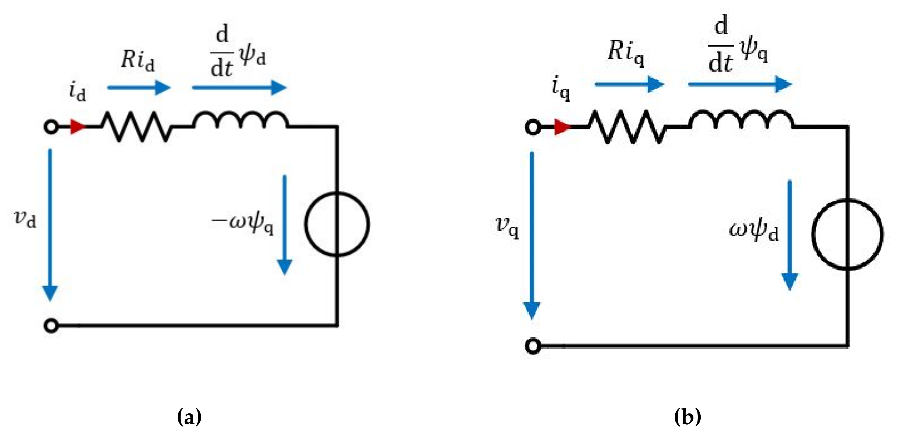
Figure 2.
Equivalent circuit model: (a) of the d-axis component; (b) of the q-axis component.
Figure 2.
Equivalent circuit model: (a) of the d-axis component; (b) of the q-axis component.
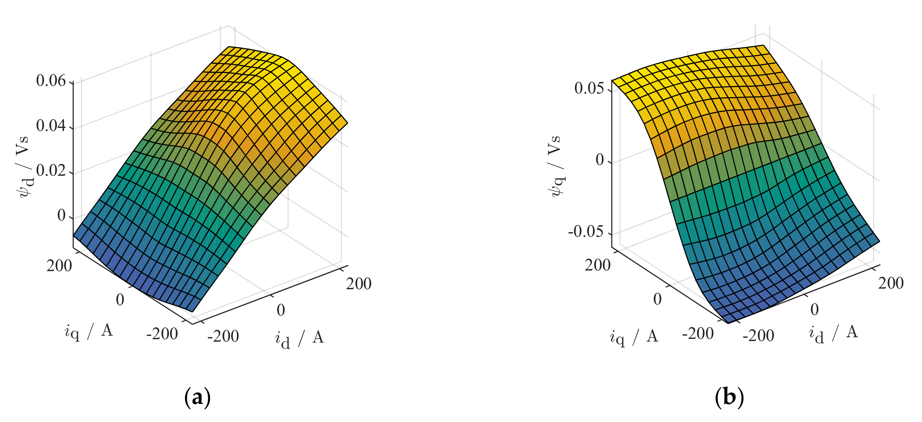
Figure 3.
Finite element analysis (FEA)-calculated flux-linkages for the used machine in simulation and for the explanations, assuming at a fixed rotor position : (a) flux-linkage of the direct-axis (b) flux-linkage of the quadrature-axis. The displayed data are of a machine with a maximum speed up to at peak power at a voltage of
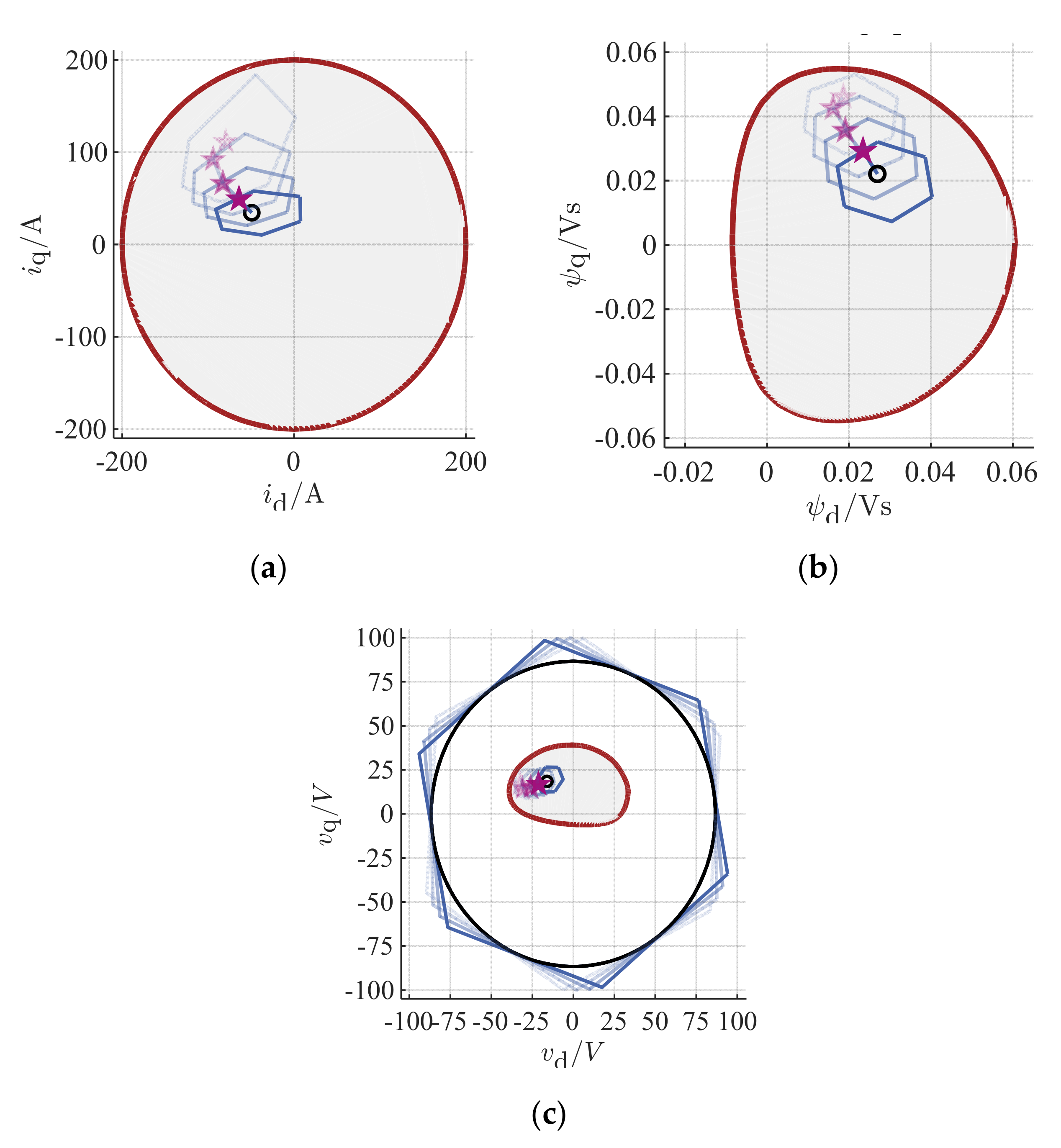
Figure 4.
Different planes: (a) current plane; (b) flux-linkage plane; (c) voltage plane. The planes (a), (b), and (c) are showing the latest operating point (small black circle). The reachable operating points inside the blue hexagon and chosen trajectory considering of each time-step and voltage hexagon (purple star). The current limitation of the machine is marked as red circle. In (c) also the rotating inverter voltage hexagon with the black inner circle is drafted.
Figure 5.
Visualization of the different control periods with sampling, prediction, and reference value calculation within the control procedure.
Figure 5.
Visualization of the different control periods with sampling, prediction, and reference value calculation within the control procedure.
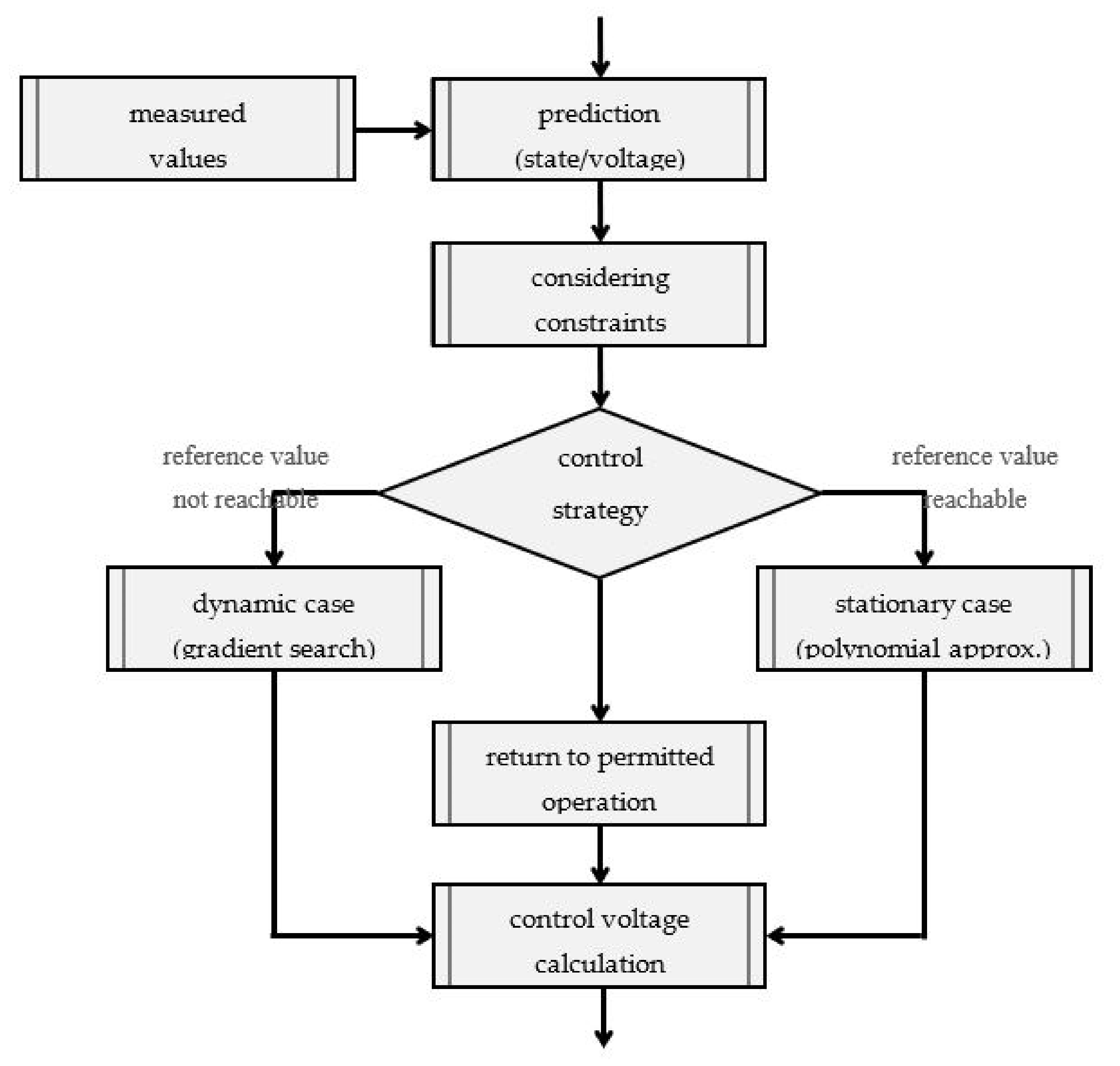
Figure 6.
Simplified diagram of the introduced control algorithm, executed for each control period.
Figure 6.
Simplified diagram of the introduced control algorithm, executed for each control period.
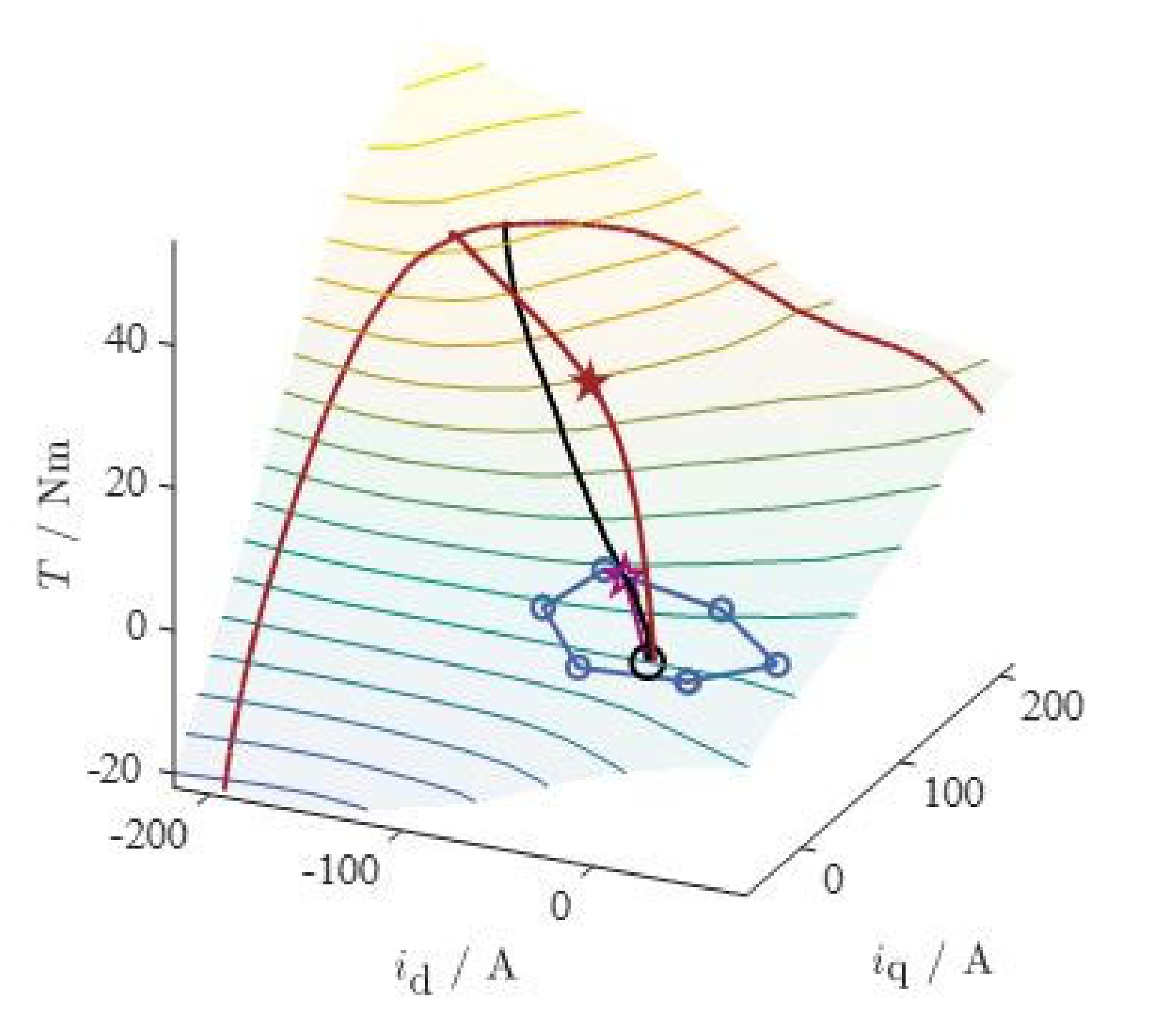
Figure 7.
Torque plane (z-axis) at present current, speed and rotor position. The gradient of the ideal reference torque trajectory is the black line, the actual torque the black circle. The boundaries are marked as blue voltage hexagon and the chosen next reference value is in purple. The reference torque is the red star with the offline calculated red MTPA trajectory for ideal steady-state operation.
Figure 8.
Calculation of the ideal reference value considering the gradient with under the certain constraints. The purple arrow shows the chosen reference value with optimal trajectory.
Figure 8.
Calculation of the ideal reference value considering the gradient with under the certain constraints. The purple arrow shows the chosen reference value with optimal trajectory.
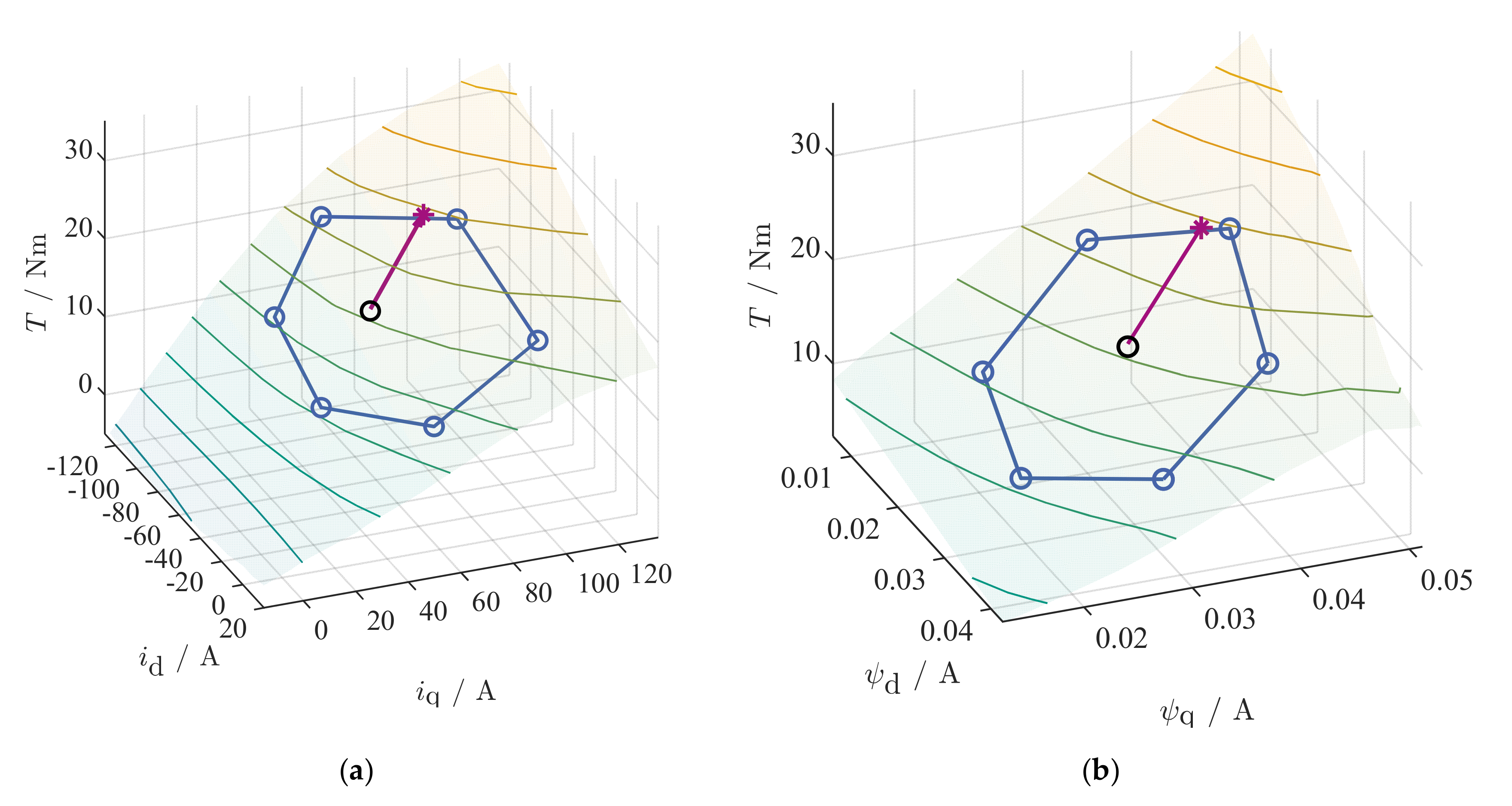
Figure 9.
Dynamic case: (
a) and (
b) torque contour lines (z-axis) and constraint area due to the applicable voltage hexagon in blue, present value as black circle. In (
a) the current plane (x- and y-axis) is shown, (
b) shows it in the equivalent flux linkage plane. The purple arrow shows the chosen reference value from
Figure 8 with fastest achievable torque for the next control period.
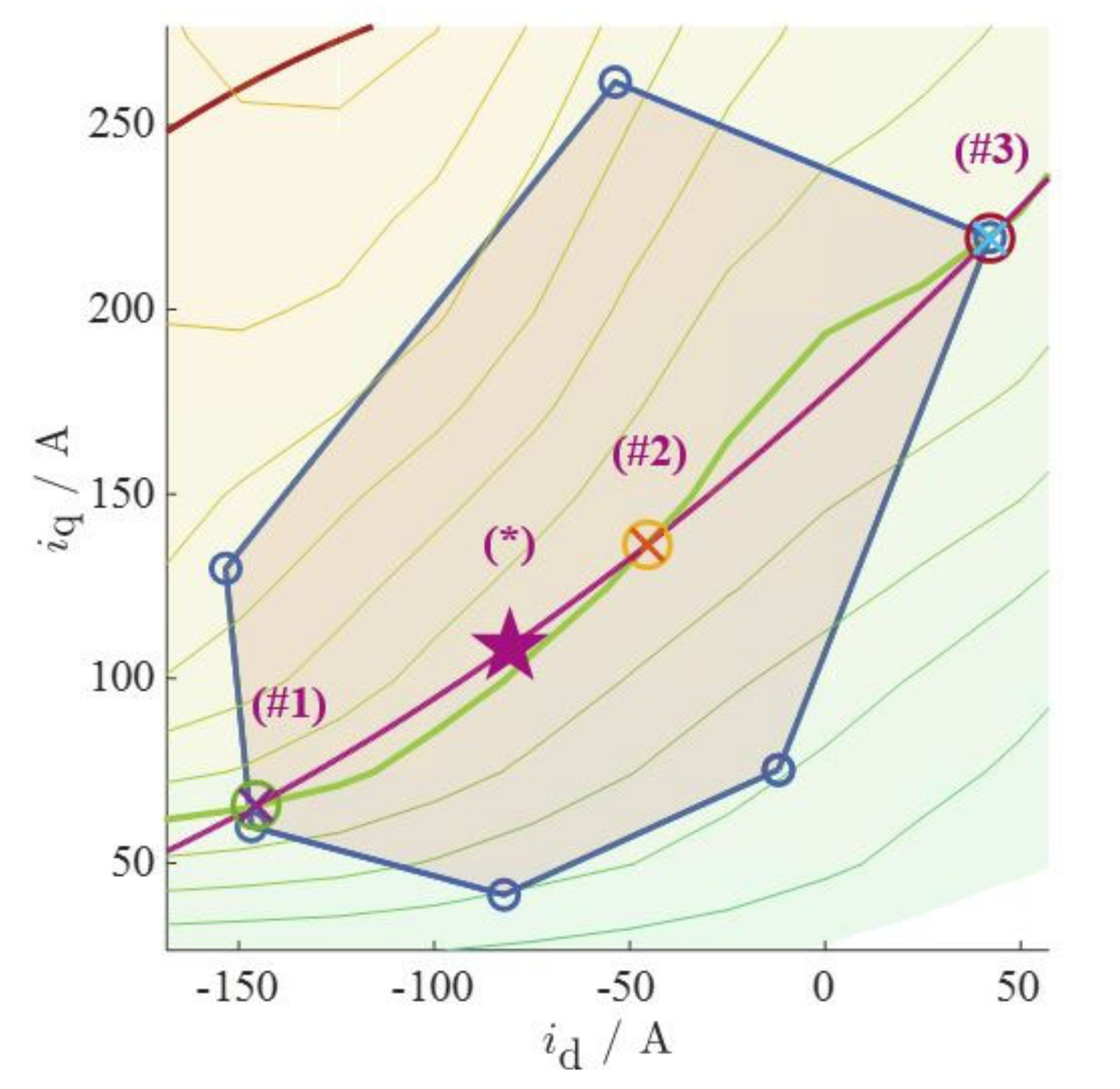
Figure 10.
Stationary case (first iterations of two): With torque contour lines (surface) and constraint area due to the applicable voltage hexagon in blue and the current limit in red. (#1) to (#3) are the values for the polynomial approximation, (*) is the solution of the first iteration of the polynomial approximation. As visible, the first approximation of the iso-torque curve (purple) does not suit the iso-torque curve, another iteration is necessary. The x- and y-axis are the direct and quadrature currents.
Figure 11.
Supporting points with intersection to the hexagonal area: Both diagrams with reference torque in black, present torque (iso-curve) in green. (
a) hexagon edges with corresponding torque intersection. As shown in
Figure 10 both hexagon edges (2 and 3) with the chosen supporting point (d- and q-current) marked with the purple cross and the green circle. (
b) shows the selection of the desired value by considering the sign and the intersection of the reference torque with the different iterations displayed with black arrows. As a result, the desired value is identified as purple cross and the green circle similar to
Figure 10.
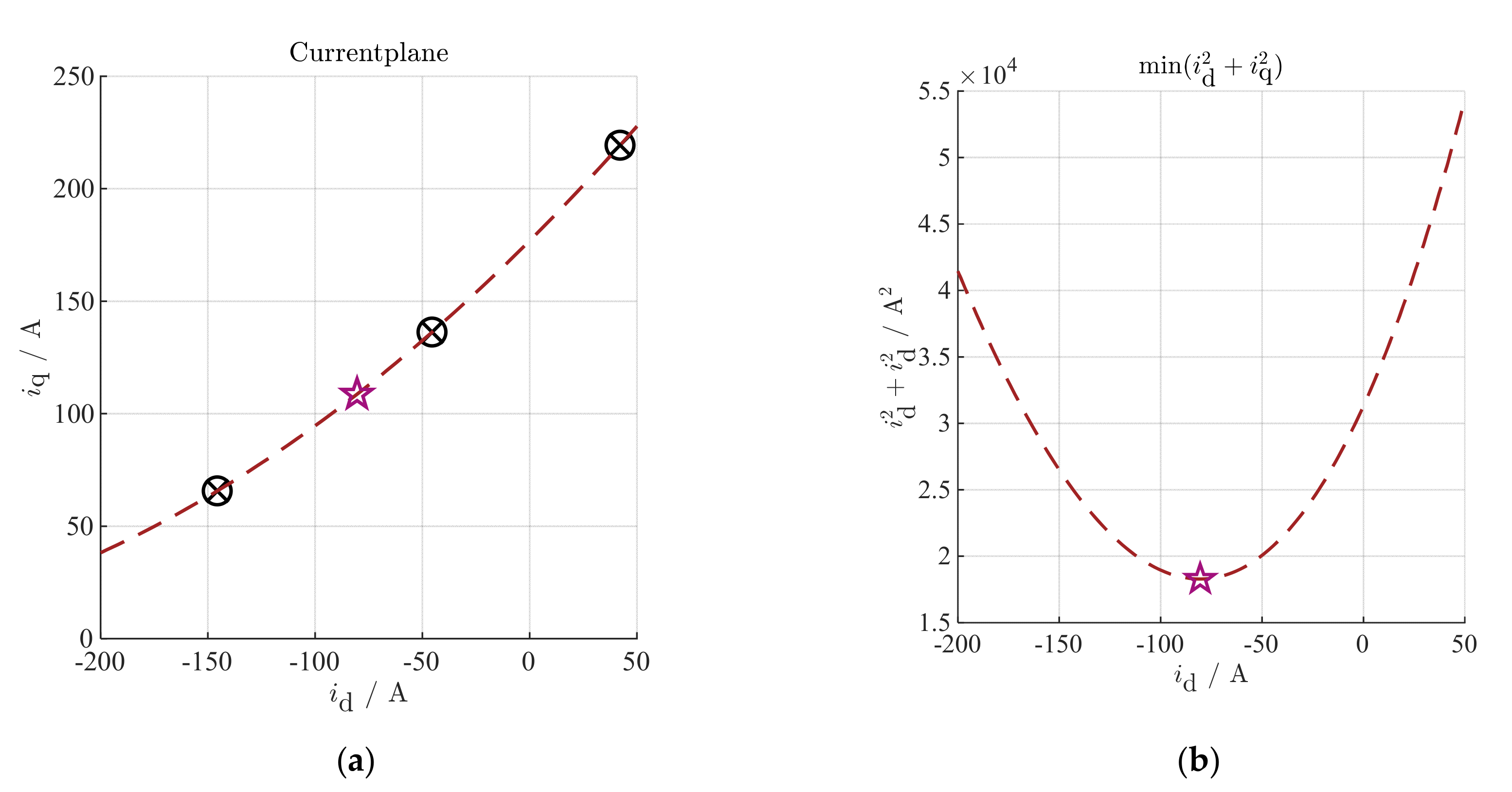
Figure 12.
Stationary case: (a) Second order polynomial approximated d- and q-current (red dashed line). The supporting points are marked with black circles, the solution of the minimization problem (b) is marked as star. (b) shows the minimization problem as described in (20).
Figure 12.
Stationary case: (a) Second order polynomial approximated d- and q-current (red dashed line). The supporting points are marked with black circles, the solution of the minimization problem (b) is marked as star. (b) shows the minimization problem as described in (20).
Figure 13.
Stationary case with two iterations: The area, which is attainable within the control period is enclosed by the blue hexagon. The current limit is displayed in red. The surface describes the machine torque. Both iterations of the polynomial approximation are shown in purple. The first iteration (
Figure 10) does not match the iso-torque curve, where the second iteration matches well with the green iso-torque curve within the range of interest.
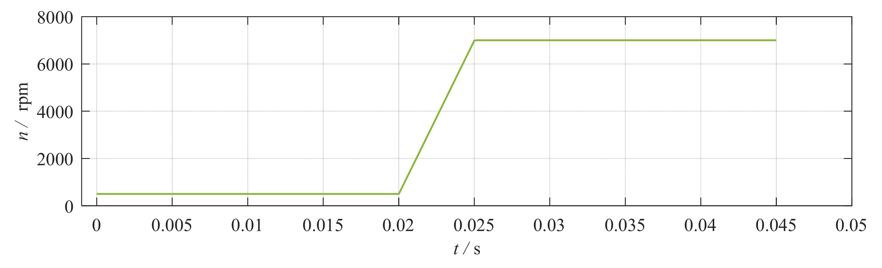
Figure 14.
Simulation setup with 500 rpm in the beginning and increased after 0.02 s to 7000 rpm for the operation at field-weakening. In
Figure 15 is the corresponding torque displayed.
Figure 14.
Simulation setup with 500 rpm in the beginning and increased after 0.02 s to 7000 rpm for the operation at field-weakening. In
Figure 15 is the corresponding torque displayed.
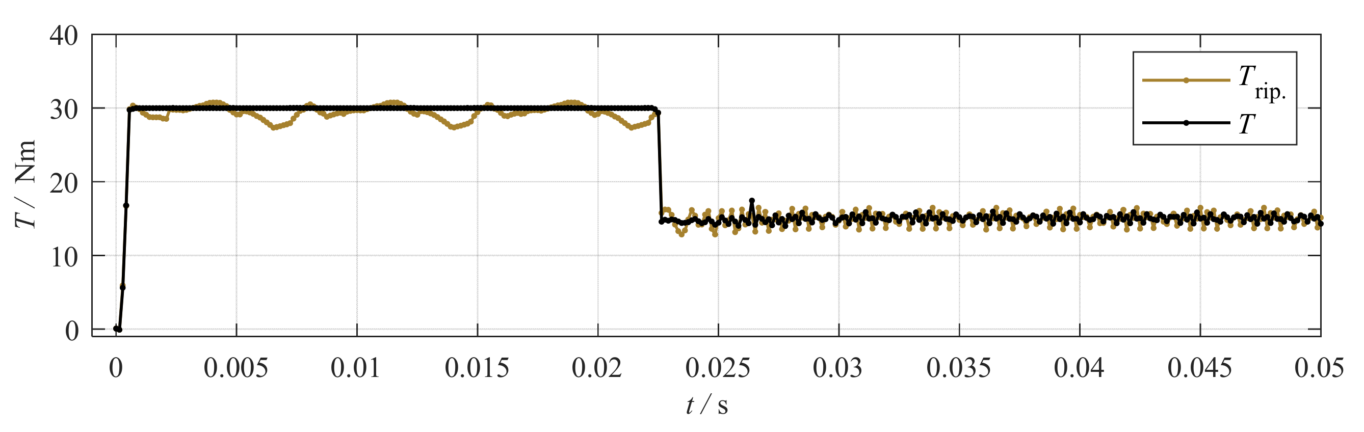
Figure 15.
Operation of the control algorithm at two different torques. The corresponding speed is shown in
Figure 14. The torque T, controlled with the introduced algorithm, is shown in black, the torque for control with equivalent constant currents
is shown in light brown.
Figure 15.
Operation of the control algorithm at two different torques. The corresponding speed is shown in
Figure 14. The torque T, controlled with the introduced algorithm, is shown in black, the torque for control with equivalent constant currents
is shown in light brown.
Figure 16.
Simulation of the trajectory in red at 30 Nm and 500 rpm, with the red dots at dynamic operation and the red crosses at stationary operation. In blue at 15 Nm and 7000 rpm, with the blue dots at dynamic operation and the blue crosses at stationary operation. The orange crosses show the behavior during changing the speed.
Figure 17.
Torque control with a fundamental predictive control algorithm and pre-calculated reference values in (b) the controlled currents to the corresponding torque (a) are displayed. In (c) the torque of the introduced algorithm is shown in brown. The minimized torque ripple is displayed black. (d) shows the corresponding online calculated currents including the current ripple needed for the minimization of the torque ripple. The simulations were done at 600 rpm rotor speed.
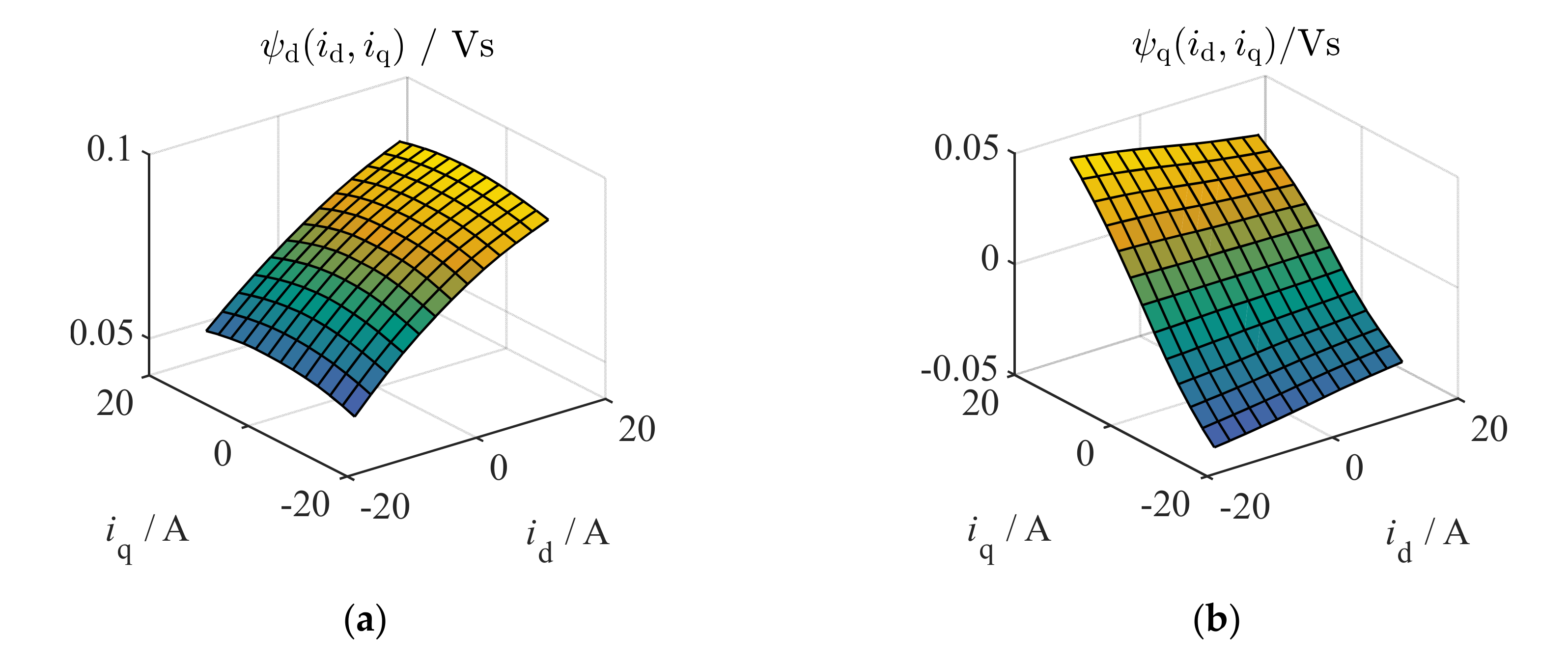
Figure 18.
Measured/estimated flux-linkages of the device under test at the test-bench, assuming at a fixed rotor position : (a) flux-linkage of the direct-axis (b) flux-linkage of the quadrature-axis.
Figure 18.
Measured/estimated flux-linkages of the device under test at the test-bench, assuming at a fixed rotor position : (a) flux-linkage of the direct-axis (b) flux-linkage of the quadrature-axis.
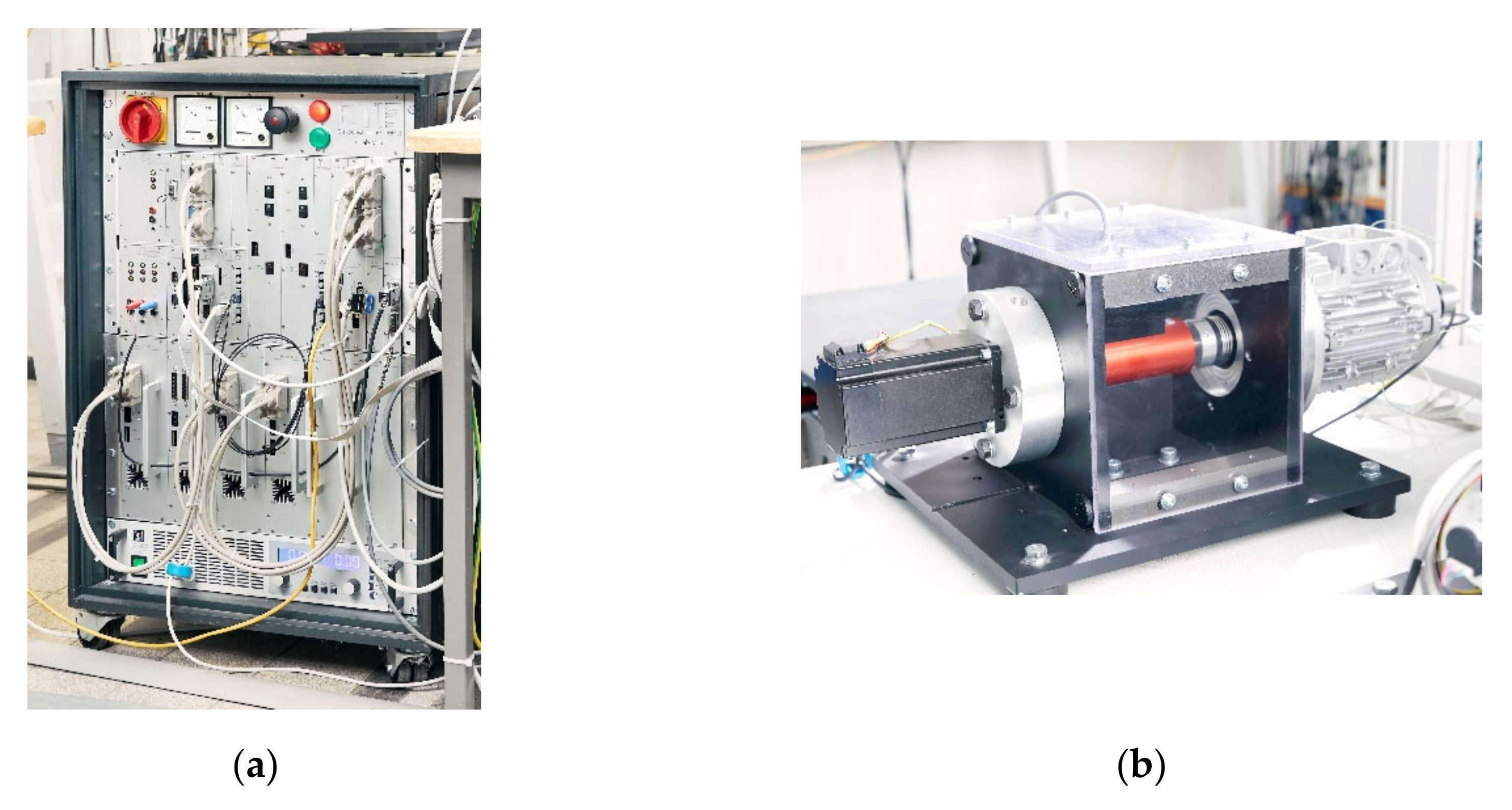
Figure 19.
Test-bench setup: (a) Testbench cabinet with inverters and signal processing; (b) mechanical assembly of device under test and load machine (Source: Amadeus Bramsiepe, KIT).
Figure 19.
Test-bench setup: (a) Testbench cabinet with inverters and signal processing; (b) mechanical assembly of device under test and load machine (Source: Amadeus Bramsiepe, KIT).
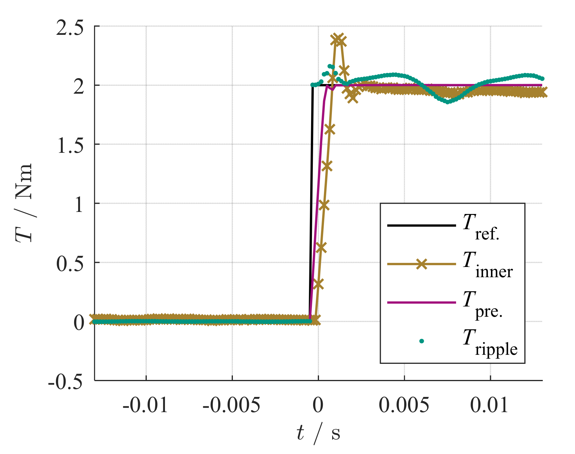
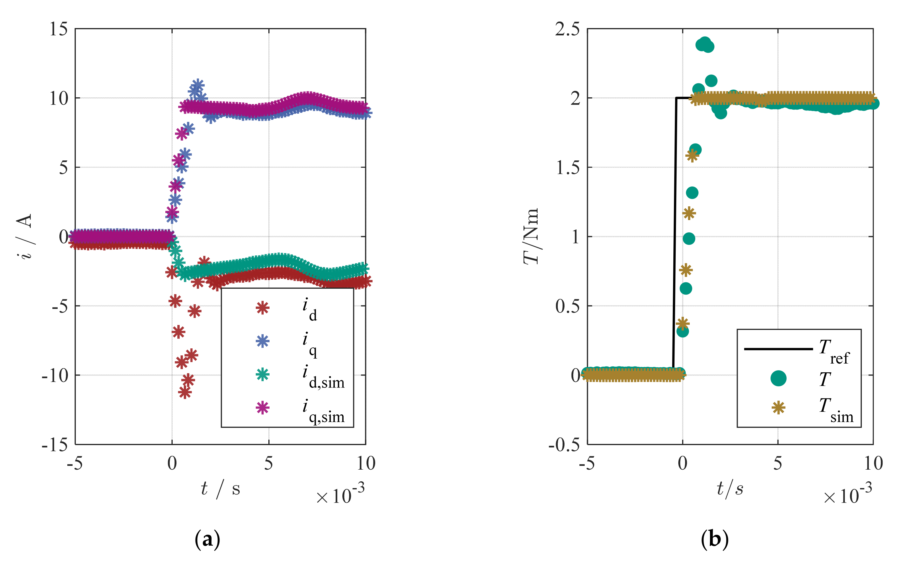
Figure 20.
Torque step from zero torque to at . The reference torque is thereby displayed black, the present inner torque (according Equation (5)) calculated as describe before is brown. The predicted torque used in the control is shown as purple line. The torque in this operational point, controlled with equivalent constant currents (as is done in fundamental approaches without torque ripple compensation) is shown as green dashed line.
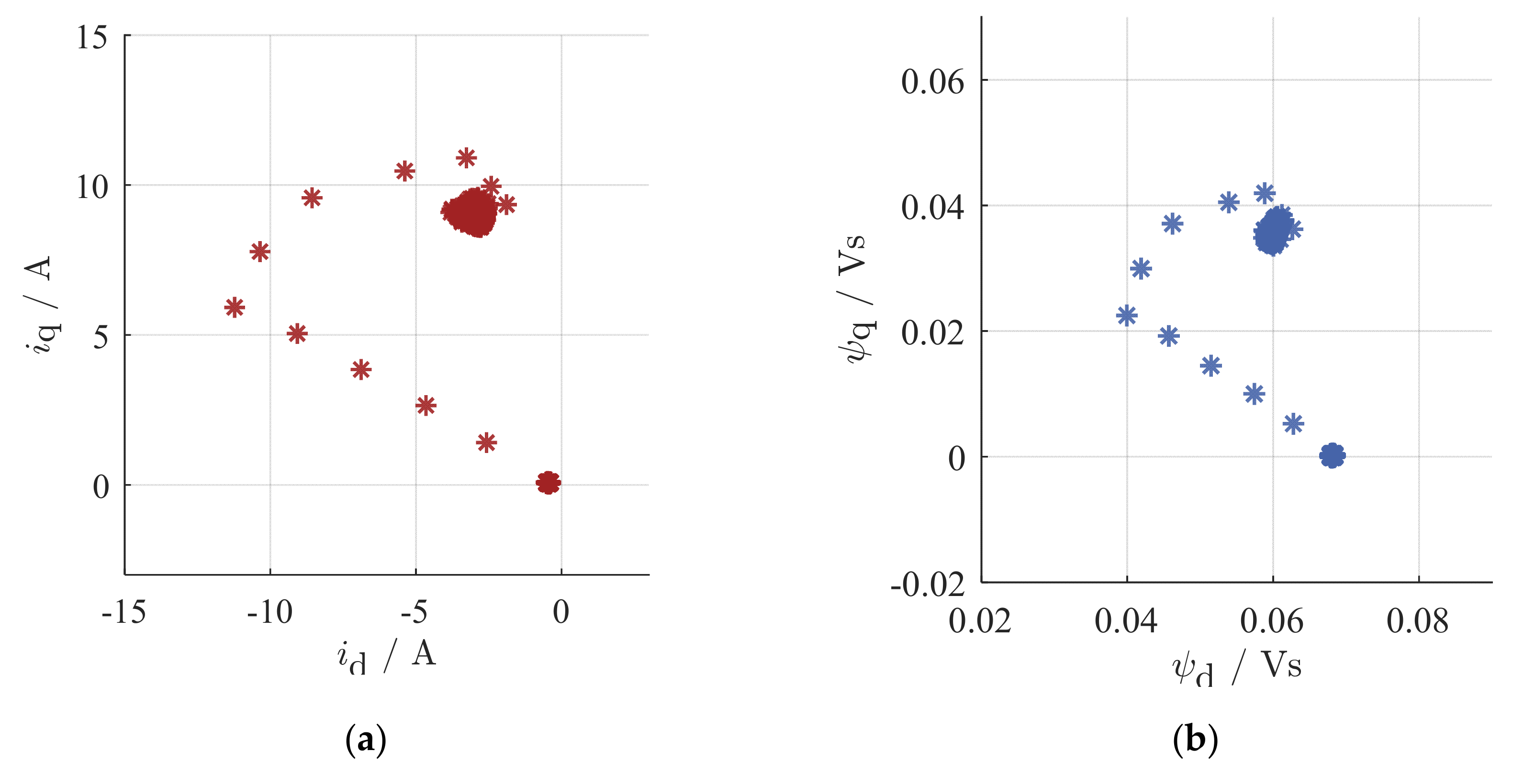
Figure 21.
Current plane (a) and flux-linkage plane (b) with the currents/flux-linkages at each time step. The values form bottom right to the left show the gradient search algorithm. After the intersection with the iso-torque curve the stationary case is applied. The heap of the values is due to the stationary torque ripple compensation.
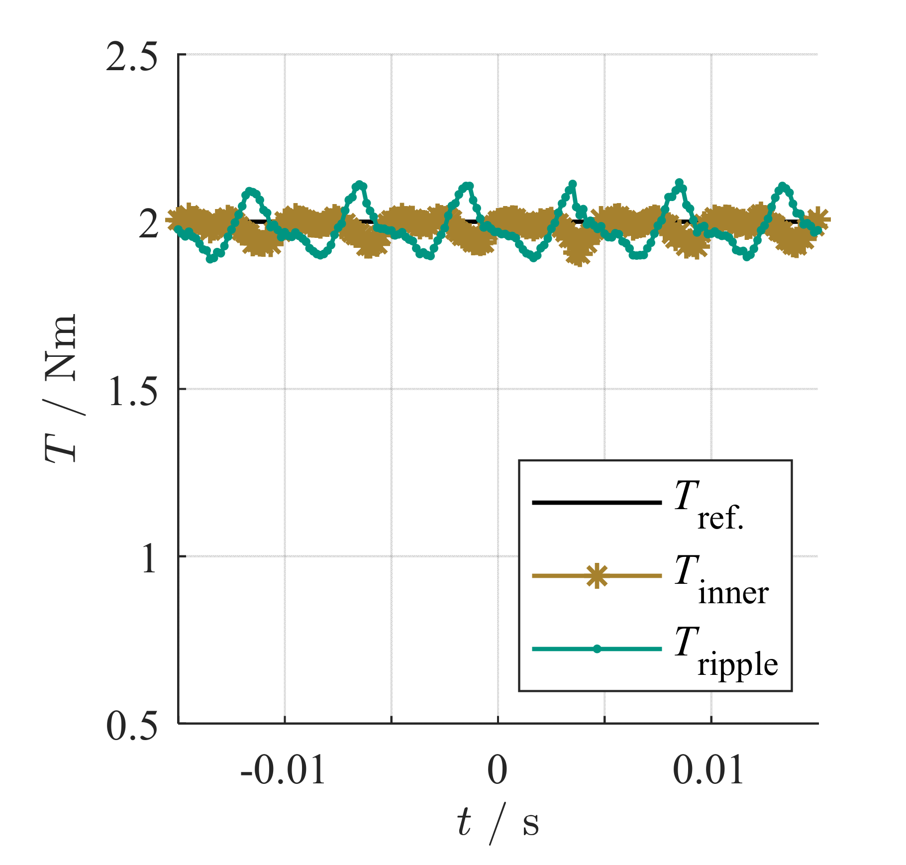
Figure 22.
Stationary operation close to the nominal speed with at . In brown: the inner torque applied by the introduced control. In green the torque with uncompensated ripple, controlled with equivalent constant. Black shows the reference torque.
Figure 22.
Stationary operation close to the nominal speed with at . In brown: the inner torque applied by the introduced control. In green the torque with uncompensated ripple, controlled with equivalent constant. Black shows the reference torque.
Figure 23.
Measurement and equivalent simulation of (a) current response (measurement in green and purple, simulation in red and blue) and (b) torque response (measurement in brown, reference torque in black and simulation in green) at a rotor speed of 500 rpm.
Figure 23.
Measurement and equivalent simulation of (a) current response (measurement in green and purple, simulation in red and blue) and (b) torque response (measurement in brown, reference torque in black and simulation in green) at a rotor speed of 500 rpm.
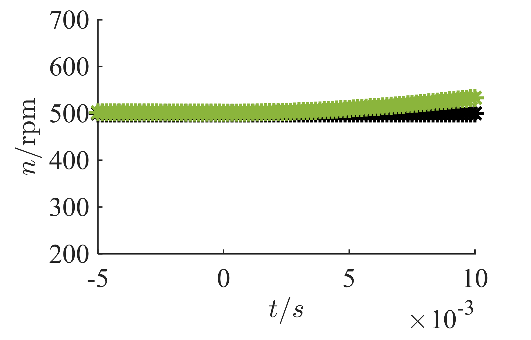
Figure 24.
Rotor speed of the measurement in green and constant rotor speed of 500 rpm in the simulation.
Figure 24.
Rotor speed of the measurement in green and constant rotor speed of 500 rpm in the simulation.
Table 1.
Main quantities of the device under test.
Table 1.
Main quantities of the device under test.
| Quantities | Symbol | Value |
|---|
| Maximum voltage | | |
| Maximum current | | |
| Nominal speed | | |
| Nominal torque | | |
| Permanent magnet flux-linkage | | |
| Stator resistance | | |

 ,
, 


