Numerical Investigation of the Effect of Partially Propped Fracture Closure on Gas Production in Fractured Shale Reservoirs

Abstract

Nonuniform proppant distribution is fairly common in hydraulic fractures, and different closure behaviors of the propped and unpropped fractures have been observed in lots of physical experiments. However, the modeling of partially propped fracture closure is rarely performed, and its effect on gas production is not well understood as a result of previous studies. In this paper, a fully coupled fluid flow and geomechanics model is developed to simulate partially propped fracture closure, and to examine its effect on gas production in fractured shale reservoirs. Specifically, an efficient hybrid model, which consists of a single porosity model, a multiple porosity model and the embedded discrete fracture model (EDFM), is adopted to model the hydro-mechanical coupling process in fractured shale reservoirs. In flow equations, the Klinkenberg effect is considered in gas apparent permeability, and adsorption/desorption is treated as an additional source term. In the geomechanical domain, the closure behaviors of propped and unpropped fractures are described through two different constitutive models. Then, a stabilized extended finite element method (XFEM) iterative formulation, which is based on the polynomial pressure projection (PPP) technique, is developed to simulate a partially propped fracture closure with the consideration of displacement discontinuity at the fracture interfaces. After that, the sequential implicit method is applied to solve the coupled problem, in which the finite volume method (FVM) and stabilized XFEM are applied to discretize the flow and geomechanics equations, respectively. Finally, the proposed method is validated through some numerical examples, and then it is further used to study the effect of partially propped fracture closures on gas production in 3D fractured shale reservoir simulation models. This work will contribute to a better understanding of the dynamic behaviors of fractured shale reservoirs during gas production, and will provide more realistic production forecasts.

1. Introduction

In the last decade, the shale gas industry has received worldwide attention [1,2,3]. Horizontal drilling [4] and hydraulic fracturing [5,6,7,8,9,10] are two key techniques for economically improving the production of shale reservoirs. Compared with conventional fracturing techniques, the liquid nitrogen technique [8,9,10] has its unique advantages for fracturing hard and high-temperature formations. During the hydraulic fracturing treatment, large amounts of fluid and proppants are injected into the shale formation to create propped fractures which act as conductive paths for the fluid flowing from the formation to the wellbore [11]. After hydraulic fracturing, shale gas reservoirs with multiscale fractures usually exhibit high early production rates, but show dramatic production declines during the late period of reservoir depletion [12]. This may be partially attributed to the closure of hydraulic fractures, thus some new methods, such as injecting silica proppants or coal fines, have been developed to prevent the closure of hydraulic fractures [13]. On the other hand, hydraulic fractures usually contain propped and unpropped fractures, and they exhibit different closure behaviors [14,15,16,17]. Specifically, the closure of propped fractures strongly depends on the proppant deformation and embedment [17], while the closure of unpropped fractures is mainly affected by the geometry of fracture surfaces [15]. Moreover, different closure behaviors could lead to different stress-dependent conductivity values for propped and unpropped fractures, which has a significant impact on the shale gas production. Therefore, in order to accurately simulate the gas production behavior in fractured shale reservoirs, it is necessary to consider the effect of partially propped fracture closure [15,18].

Some related previous studies are briefly summarized here. Cipolla et al. [19,20] and Sierra et al. [21] studied the effects of proppant distribution (e.g., proppant settling), unpropped fracture conductivity and high-conductivity arches on gas well performance, but the fracture closure and stress-dependent fracture conductivity were not taken into consideration. Yu et al. [22,23] developed a reservoir simulation approach to study the effects of proppant distribution and stress-dependent fracture conductivity on gas well performance. Similarly, Lee et al. [12] also developed a numerical model to investigate the combined effect of proppant placement and fracture closure on gas production. Liu et al. [14,18] obtained the post-closure geometry of a partially propped fracture through geomechanical simulations, and then incorporated it into the flow simulations to study the effects of proppant distribution, fracture closure and gravity segregation on water flowback and gas production. However, these studies are mainly focused on the fluid flow aspects, while the geomechanical effects have not been considered in detail. That is, they assumed that the total stress field remains constant during flow simulations, and correlated the fracture permeability to the reservoir pressure to simplify the geomechanical effects. In order to accurately consider the geomechanical effects, Zhou et al. [15] and Zheng et al. [24,25] developed hydro-mechanical coupling models to investigate the effects of fracture closure and nonuniform proppant distribution on gas production. However, the displacement discontinuity at hydraulic fractures, which has an important influence on the evolution of the total stress acting on hydraulic fractures, was neglected in these studies.

In this paper, a fully coupled fluid flow and geomechanics model is developed to simulate the partially propped fracture closure and to examine its effect on gas production in fractured shale reservoirs. This paper is organized as follows: The hybrid model [3], which consists of a single porosity model, a multiple porosity model and the EDFM [26,27,28], is presented in Section 2. In Section 3, the stabilized XFEM iterative formulation based on the PPP technique [29,30,31] is developed, and then the modified fixed-stress sequential implicit method [32,33] is applied to solve the coupled problem, in which the FVM [34,35,36,37] and stabilized XFEM are used to discrete the flow and geomechanics equations, respectively. In Section 4, we validate the proposed method through some numerical examples, and then it is further used to investigate the effects of partially propped fracture closure on gas production in 3D fractured shale reservoir simulation models. The conclusions are provided in Section 5.

2. Mathematical Model Descriptions

As shown in Figure 1, a shale reservoir usually possesses hydraulic fractures and natural fractures due to hydraulic fracturing, and it can be divided into two regions—one is the stimulated reservoir volume (SRV), which consists of natural fractures, the shale matrix and hydraulic fractures, and the other is the region with little fractures outside the SRV. In this study, an efficient hybrid model is adopted to simulate the gas production in such a shale reservoir. Specifically, the single porosity model is applied in the outside region, while a multiple porosity model is used inside the SRV to consider both the natural fractures and shale matrix. Meanwhile, hydraulic fractures are modeled explicitly by use of the EDFM.

2.1. Fluid-Governing Equations

In this study, we assume that gas is stored as a free phase in the fractures, while it is stored as both free and adsorbed phases in the shale matrix. The governing equation for isothermal single-phase gas flow is obtained from the mass conservation law [38], and its general integral form is:

$$\frac{\partial }{\partial t}{\displaystyle {\int }_{\mathsf{\Omega }}A} \mathrm{d}\mathsf{\Omega }+{\displaystyle {\int }_{\mathsf{\Gamma }}\mathit{F}}·\mathit{n} \mathrm{d}\mathsf{\Gamma } = {\displaystyle {\int }_{\mathsf{\Omega }}q} \mathrm{d}\mathsf{\Omega }$$

(1)

where n is the unit normal vector of boundary Γ, and A, F and q are the mass accumulation, mass flux and source terms on domain Ω, respectively. The mass accumulation is expressed as:

$$A=\varphi {\rho }_{\mathrm{g}}+\left(1-\varphi \right)m$$

(2)

where ϕ is the Lagrange porosity, and its definition can be found in references [3,28]. ρ_g is the gas density, and m is the mass of gas adsorbed per solid volume (only exists for matrix), and it is determined according to the Langmuir’s isotherm [39,40] as a function of gas pressure:

$${\rho }_g=\frac{pM}{ZRT}, m={\rho }_{\mathrm{r}}{\rho }_{\mathrm{gstd}}{V}_{\mathrm{L}}\frac{p/Z}{p_{\mathrm{L}}+p/Z}$$

(3)

where p is the gas pressure, M is the gas molar mass, Z is the gas compression factor, R is the universal gas constant, T is the reservoir temperature, ρ_r is the rock bulk density, ρ_gstd is the gas density at standard condition, and V_L and P_L are the Langmuir volume and Langmuir pressure, respectively.

The mass flux term in Equation (1) is given by:

$$\mathit{F}=-{\rho }_{\mathrm{g}}\frac{k}{\mu }\left(1+\frac{b}{p}\right)\left(\nabla p-{\rho }_{\mathrm{g}}\mathrm{g}\nabla D\right)$$

(4)

where k is the absolute permeability, µ is the gas viscosity, g is the gravity acceleration, D is the depth, and b is the Klinkenberg factor, which incorporates the gas-slippage effect in gas-flow models by modifying the absolute permeability as a function of gas pressure [38,41]

$$b=\frac{p\mu c{D}_{\mathrm{k}}}{k}, c=\frac{1}{p}-\frac{1}{Z}\left(\frac{\partial Z}{\partial p}\right), D_k=\frac{4kZ}{2.81708\sqrt{k/\varphi }}\sqrt{\frac{\pi RT}{2M}}$$

(5)

where c is the gas compressibility, and D_k is the Knudsen diffusion coefficient for real gas [3].

The fluid flow boundary conditions are

$$\mathit{v}·{\mathit{n}}_q=\overline{q} \mathrm{on} {\mathsf{\Gamma }}_q,p=\overline{p} \mathrm{on} {\mathsf{\Gamma }}_p$$

(6)

where v is the flow rate, and $\overline{q}$ and $\overline{p}$ are the prescribed flow rate and pressure on boundaries Γ_q and Γ_p, respectively, as shown in Figure 2. n_q is the unit normal vector of Γ_q.

2.2. Geomechanics-Governing Equations

The governing equation for solid deformation under the assumption of quasi-static infinitesimal deformation is given as [42] (the sign convention of continuum mechanics is adopted here):

$$\nabla ·\mathit{\sigma }+{\rho }_{\mathrm{b}}\mathbf{g}=\mathbf{0}$$

(7)

where σ is the total stress tensor, and ρ_b is the bulk density. In the hybrid model, the total stress tensor is defined as [3]

$$\mathit{\sigma }=\{\begin{array}{ll}\mathit{C}\mathit{\epsilon }-\alpha p\mathbf{I},& \mathrm{outside} \mathrm{the} \mathrm{SRV}\\ {\mathit{C}}_{\mathrm{up}}\mathit{\epsilon }+{\displaystyle {\sum }_l{K}_{\mathrm{dr}}{b}_l}{p}_l\mathbf{I},& \mathrm{in} \mathrm{the} \mathrm{SRV}\end{array}$$

(8)

where C and α are the elasticity tensor and Biot coefficient of the shale matrix, I is the identity tensor, C_up and K_dr are the upscaled elasticity tensor and drained bulk modulus at the level of gridblock, b is a coupling coefficient, and the subscript l indicates the l-th sub-gridblock within each matrix gridblock. Detailed definitions of C_up, K_dr and b_l can be found in reference [3]. The strain tensor ε is given as the symmetric gradient of displacement vector u from infinitesimal deformation:

$$\mathit{\epsilon }=\frac{1}{2}\left(\nabla \mathit{u}+{\nabla }^{\mathrm{T}}\mathit{u}\right)$$

(9)

where $\nabla$ indicates the gradient operator, and the superscript T indicates transpose.

The geomechanics boundary conditions are

$$\mathit{\sigma }·{\mathit{n}}_{\mathrm{t}}=\overline{\mathit{t}} \mathrm{on} {\mathsf{\Gamma }}_{\mathit{t}}, \mathit{u}=\overline{\mathit{u}} \mathrm{on} {\mathsf{\Gamma }}_u$$

(10)

$$\mathit{\sigma }·{\mathit{n}}_{\mathrm{HF}}=-\left(p_{\mathrm{HF}}+p_{\mathrm{s}}\right)·{\mathit{n}}_{\mathrm{HF}} \mathrm{on} {\mathsf{\Gamma }}_{\mathrm{HF}}$$

(11)

where $\overline{\mathit{t}}$ and $\overline{\mathit{u}}$ are the prescribed traction and displacement on boundaries Γ_t and Γ_u, respectively, n_t is the unit normal vector of Γ; p_HF is the gas pressure in the fracture, which is exerted on the inner fracture faces Γ_HF, ${\mathit{n}}_{\mathrm{HF}}$ is the unit normal vector of Γ_HF pointing to Ω⁺ with ${\mathit{n}}_{\mathrm{HF}}={\mathit{n}}_{\mathrm{HF}}^{-}=-{\mathit{n}}_{\mathrm{HF}}^{+}$, as shown in Figure 2, and p_s is the effective stress exerted on the inner fracture faces, which is caused by the compression of proppants (propped) or the contact of fracture faces (unpropped), and its formula will be given in Equations (12) and (13).

2.3. Constitutive Relations

In this study, we assume that a hydraulic fracture is represented by two parallel plates, and the closure of the propped hydraulic fractures mainly depends on proppant deformation, thus its general constitutive model is defined as

$$p_{\mathrm{s}}=\{\begin{array}{ll}{f}_{\mathrm{s}}\left({\epsilon }_{\mathrm{s}}\right),& {\epsilon }_{\mathrm{s}}>0\\ 0,& {\epsilon }_{\mathrm{s}}\le 0\end{array}$$

(12)

where f_s indicates the nonlinear stress–strain relationship of proppant deformation, and it can be obtained from mechanical experiments, ${\epsilon }_{\mathrm{s}}=-〚\mathit{u}〛·{\mathit{n}}_{\mathrm{HF}}/d_{\mathrm{HF0}}$ is the normal proppant strain, $〚\mathit{u}〛={\mathit{u}}^{+}-{\mathit{u}}^{-}$ represents the displacement difference between fracture faces, and d_HF0 is the initial fracture aperture.

For the closure of unpropped hydraulic fractures, a constitutive model modified from the self-contact condition and penalty method [43] is written as

$$p_{\mathrm{s}}=\{\begin{array}{ll}-E_{\mathrm{n}}{d}_{\mathrm{HF}},& d_{\mathrm{HF}}<0\\ 0,& d_{\mathrm{HF}}\ge 0\end{array}$$

(13)

where $d_{\mathrm{HF}}=d_{\mathrm{HF0}}+〚\mathit{u}〛·{\mathit{n}}_{\mathrm{HF}}$ is the residual fracture aperture, and E_n≫1 is a normal penalty parameter. This constitutive model allows for a small interpenetration of the fracture faces because of the finite value of E_n [43].

Based on the Kozeny–Carman equation [44,45], the dynamic permeability of matrix k_m can be written as

$$k_{\mathrm{m}}=k_{\mathrm{m}0}{\left(\frac{{\varphi }_{\mathrm{m}}}{{\varphi }_{\mathrm{m}0}}\right)}^3{\left(\frac{1-{\varphi }_{\mathrm{m}0}}{1-{\varphi }_{\mathrm{m}}}\right)}^2$$

(14)

where k_m and ϕ_m are the matrix permeability and porosity, respectively. The subscript 0 represents the initial state. The dynamic permeability of natural fractures is [3]

$$k_{\mathrm{f}}=k_{\mathrm{f0}}{\left(1+\frac{K_{\mathrm{dr}}}{K_{\mathrm{f}}}{\epsilon }_{\mathrm{v}}\right)}^3{\left(1+{\epsilon }_{\mathrm{v}}\right)}^{-2}$$

(15)

where K_f is the drained bulk modulus of natural fractures, and ε_v is the volumetric strain of a gridblock.

According to the parallel plate assumption and cubic law [46,47,48], the dynamic permeability of unpropped hydraulic fractures can be written as

$$k_{\mathrm{HF}}=\frac{d_{\mathrm{HF}}^2}{12}$$

(16)

A number of experimental results have reported that the dynamic permeability of propped hydraulic fractures is related to effective stress [49,50]

$$k_{\mathrm{HF}}=f_{\mathrm{k}}\left(p_{\mathrm{s}}\right)$$

(17)

where f_k indicates the relationship between fracture permeability and effective stress, and it can be obtained from conductivity experiments [51,52,53]. In this study, only the normal deformation of hydraulic fractures is considered, and the shear slip and related dilation will be included in future publications.

3. Numerical Schemes

The mixed space discretization is applied in this study. The space discretization for fluid flow is achieved by using the FVM, in which pressure is located at the elements’ centers. On the other hand, the stabilized XFEM is employed for geomechanics, where the displacement vectors are located at grid vertices. The geometry discretization is achieved by using orthogonal grids, and hydraulic fractures are discretized according to the intersections of hydraulic fractures and orthogonal grids. Besides, the nested grids based on the improved MINC method are generated inside each matrix block in the SRV. More details about the geometry discretization can be found in reference [3].

3.1. Flow Equations Discretization

The FVM is applied to discretize the gas flow-governing equation (i.e., Equation (1)), and the standard first-order approximation is used for time discretization, while accumulation and mass flux terms are evaluated fully implicitly. The residual of Equation (1) can be written as:

$$R_i^{n+1}=\left[{\left(\varphi {\rho }_{\mathrm{g}}+\left(1-\varphi \right)m\right)}_i^{n+1}-{\left(\varphi {\rho }_{\mathrm{g}}+\left(1-\varphi \right)m\right)}_i^n\right]\frac{V_i}{\mathsf{\Delta }t}-{\displaystyle \sum _{j\in G_i}{\left(\rho \lambda \right)}_{ij+1/2}^{n+1}{T}_{ij}\left(p_j^{n+1}-p_i^{n+1}\right)}-q_i^{n+1}{V}_i$$

(18)

where n is the time level, i and j are element numbers, Δt is the time step, V is the element volume, G_i is the adjacent element set of element I, ij + 1/2 represents the upstream weight value on the interface between elements i and j, λ = 1/µ is the gas mobility, and T_ij is the transmissibility between elements i and j, defined as

$$T_{ij}=\frac{A_{ij}{k}_{ij+1/2}}{d_i+d_j}$$

(19)

where A_ij is the interface area, d_i and d_j are vertical distances from cell center to the interface, and k_ij+1/2 is the harmonic-weighted permeability. To include the Klinkenberg effect on gas flow, the permeability in Equation (19) should be evaluated as (k(1 + b/p))_ij+1/2. More details about the calculation of T_ij in different domains can be found in reference [3].

Finally, Equation (18) can be solved by using the Newton–Raphson method, which iterates until convergence

$$\frac{\partial R_i^{\mathit{n}+1}\left(p_i^{\mathit{n}+1}\right)}{\partial p}\delta p_{i+1}^{\mathit{n}+1}=-R_i^{\mathit{n}+1}\left(p_i^{\mathit{n}+1}\right), p_{i+1}^{\mathit{n}+1}=\delta p_{i+1}^{\mathit{n}+1}+p_i^{\mathit{n}+1}$$

(20)

where i denotes the iterative step within one time step.

3.2. Geomechanics Equations Discretization

The governing equation for solid deformation is discretized by using the XFEM. The weak form of Equation (7) after incorporating Equations (8) and (11) is given as [44]

$${\displaystyle {\int }_{\mathsf{\Omega }}\delta \mathit{\epsilon }}:{\mathit{C}}_a\mathit{\epsilon } \mathrm{d}\mathsf{\Omega }={\displaystyle {\int }_{\mathsf{\Omega }}\delta \mathit{\epsilon }}:p_a\mathbf{I} \mathrm{d}\mathsf{\Omega }+{\displaystyle {\int }_{{\mathsf{\Gamma }}_{\mathrm{HF}}}〚\delta \mathit{u}〛\left(p_{\mathrm{HF}}+p_{\mathrm{s}}\right)}\cdot n_{\mathrm{HF}} \mathrm{d}\mathsf{\Gamma }+{\displaystyle {\int }_{\mathsf{\Omega }}\delta \mathit{u}}\cdot {\rho }_{\mathrm{b}}\mathbf{g} \mathrm{d}\mathsf{\Omega }+{\displaystyle {\int }_{\mathsf{\Gamma }\mathrm{t}}\delta \mathit{u}}\cdot \overline{\mathit{t}} \mathrm{d}\mathsf{\Gamma }$$

(21)

where C_a indicates C and C_up for the regions outside SRV and in SRV, respectively, and p_a = p in the region outside SRV, while we define p_a of a gridblock in SRV as

$$p_a=-{\displaystyle {\sum }_l{K}_{\mathrm{dr}}}{b}_l{p}_l$$

(22)

The equal-order linear interpolation of displacement does not satisfy the discrete LBB condition [30], and this leads to the unstable approximation (i.e., displacement oscillation) for Equation (21). Therefore, the PPP technique [30] is used to establish a stabilized XFEM formulation by adding a stabilizing term to Equation (21)

$$\begin{array}{c}{\displaystyle {\int }_{\mathsf{\Omega }}\delta \mathit{\epsilon }}:{\mathit{C}}_a\mathit{\epsilon }\mathrm{d}\mathsf{\Omega }={\displaystyle {\int }_{\mathsf{\Omega }}\delta \mathit{\epsilon }}:p_a\mathbf{I} \mathrm{d}\mathsf{\Omega }+{\displaystyle {\int }_{{\mathsf{\Gamma }}_{\mathrm{HF}}}〚\delta \mathit{u}〛\left(p_{\mathrm{HF}}+p_{\mathrm{s}}\right)}·{\mathit{n}}_{\mathrm{HF}} \mathrm{d}\mathsf{\Gamma }+{\displaystyle {\int }_{\mathsf{\Omega }}\delta \mathit{u}}·{\rho }_b\mathbf{g} \mathrm{d}\mathsf{\Omega }+{\displaystyle {\int }_{\mathsf{\Gamma }t}\delta \mathit{u}}·\overline{\mathit{t}} \mathrm{d}\mathsf{\Gamma }\\ \underset{\mathrm{Stabilizing} \mathrm{term}}{\underbrace{-{\displaystyle {\int }_{{\mathsf{\Gamma }}_{\mathrm{HF}}}\frac{\tau }{2M}\left(\delta p_{\mathrm{s}}-\mathsf{\Pi }\delta p_{\mathrm{s}}\right)\left(p_{\mathrm{s}}-\mathsf{\Pi }{p}_{\mathrm{s}}\right)}\mathrm{d}\mathsf{\Gamma }}}\end{array}$$

(23)

where τ > 0 is a stabilization parameter [3], which typically has a dimensionless value in the order of 1.0, and M is bulk modulus, equal to K_dr in this study. Π denotes a projection operator, and its definition can be found in references [3,30].

To represent the displacement discontinuity between hydraulic fracture faces, the displacement field is approximated by adding enrichment functions to standard finite element space [54]. By substituting the enriched displacement field and test function of the displacement field into Equation (23), and satisfying the necessity that weak form should hold for all kinematically admissible test functions, Equation (23) can be written as:

$${\mathbf{f}}_{\alpha }^{\mathrm{int}}={\mathbf{f}}_{\alpha }^{\mathrm{ext}}, \alpha =u,a,b,c$$

(24)

with

$${\mathbf{f}}_{\alpha }^{\mathrm{int}}={\displaystyle {\int }_{\mathsf{\Omega }}{\left({\mathit{B}}_u^{\alpha }\right)}^{\mathrm{T}}{\mathit{C}}_a\mathit{\epsilon }\mathrm{d}\mathsf{\Omega }}$$

(25)

$$\begin{array}{c}{\mathbf{f}}_{\alpha }^{\mathrm{ext}}={\displaystyle {\int }_{\mathsf{\Omega }}{\left({\mathit{B}}_u^{\alpha }\right)}^{\mathrm{T}}}\mathbf{m}{p}_a d\mathsf{\Omega }+{\displaystyle {\int }_{{\mathsf{\Gamma }}_{\mathrm{HF}}}{〚N_u^{\alpha }〛}^{\mathrm{T}}\left(p_{\mathrm{HF}}+p_{\mathrm{s}}\right)}·{\mathit{n}}_{HF} \mathrm{d}\mathsf{\Gamma }+{\displaystyle {\int }_{\mathsf{\Omega }}{\left({\mathit{N}}_u^{\alpha }\right)}^{\mathrm{T}}}{\rho }_{\mathrm{b}}\mathbf{g}\mathrm{d}\mathsf{\Omega }+{\displaystyle {\int }_{\mathsf{\Gamma }t}{\left({\mathit{N}}_u^{\alpha }\right)}^{\mathrm{T}}}\overline{\mathit{t}} \mathrm{d}\mathsf{\Gamma }\\ \underset{\mathrm{Stabilizing} \mathrm{term}}{\underbrace{-{\displaystyle {\int }_{{\mathsf{\Gamma }}_{\mathrm{HF}}}\frac{\tau }{2M}\left(\delta p_{\mathrm{s}}-\mathsf{\Pi }\delta p_{\mathrm{s}}\right)\left(p_{\mathrm{s}}-\mathsf{\Pi }{p}_{\mathrm{s}}\right)}\mathrm{d}\mathsf{\Gamma }}}\end{array}$$

(26)

where u, a, b, and c indicate the standard and enriched DOFs, respectively, f^int and f^ext indicate internal force vector and external force vector, respectively, m = [1,1,0]^T (2D) and m = [1,1,1,0,0,0]^T (3D). Because the effective stress p_s is nonlinear, Equation (24) would be solved by using the Newton–Raphson method, and its discretized form can be written as

$$\left(\begin{array}{c}{\mathit{K}}_{uu}{\mathit{K}}_{ua}{\mathit{K}}_{ub}{\mathit{K}}_{uc}\\ {\mathit{K}}_{au}{\mathit{K}}_{aa}{\mathit{K}}_{ab}{\mathit{K}}_{ac}\\ {\mathit{K}}_{bu}{\mathit{K}}_{ba}{\mathit{K}}_{bb}{\mathit{K}}_{bc}\\ {\mathit{K}}_{cu}{\mathit{K}}_{ca}{\mathit{K}}_{cb}{\mathit{K}}_{cc}\end{array}\right)\left[\begin{array}{l}\delta {\mathit{u}}^k\\ \delta {\mathit{a}}^k\\ \delta {\mathit{b}}^k\\ \delta {\mathit{c}}^k\end{array}\right]=-\left(\begin{array}{l}{\mathit{R}}_u^{k-1}\\ {\mathit{R}}_a^{k-1}\\ {\mathit{R}}_b^{k-1}\\ {\mathit{R}}_c^{k-1}\end{array}\right)$$

(27)

where superscript k is the current iteration step, and k-1 is the previous iteration step. $R_{\alpha }={\mathbf{f}}_{\alpha }^{\mathrm{int}}-{\mathbf{f}}_{\alpha }^{\mathrm{ext}}$ indicates the residual force vector, $\delta \alpha$ is the increment of DOFs, and K is the stiffness matrix, which should be updated at each iteration step as:

$$\begin{array}{c}{\mathit{K}}_{\alpha \beta }={\displaystyle {\int }_{\mathsf{\Omega }}{\left({\mathit{B}}_u^{\alpha }\right)}^{\mathrm{T}}}{\mathit{C}}_a{\mathit{B}}_u^{\beta }\mathrm{d}\mathsf{\Omega } +{\displaystyle {\int }_{{\mathsf{\Gamma }}_{\mathrm{HF}}}\frac{{\chi }_1}{d_{\mathrm{HF0}}}{〚{\mathit{N}}_u^{\alpha }〛}^{\mathrm{T}}\left({\mathit{n}}_{\mathrm{HF}}\otimes {\mathit{n}}_{\mathrm{HF}}\right)}〚{\mathit{N}}_u^{\beta }〛\mathrm{d}\mathsf{\Gamma }\\ + \underset{\mathrm{Stabilizing} \mathrm{term}}{\underbrace{{\displaystyle {\int }_{{\mathsf{\Gamma }}_{\mathrm{HF}}}\frac{\tau }{2M}\frac{{\chi }_2}{d_{\mathrm{HF0}}^2}{\left(〚{\mathit{N}}_u^{\alpha }〛-\mathsf{\Pi }〚{\mathit{N}}_u^{\alpha }〛\right)}^{\mathrm{T}}\left({\mathit{n}}_{\mathrm{HF}}\otimes {\mathit{n}}_{\mathrm{HF}}\right)\left(〚{\mathit{N}}_u^{\beta }〛-\mathsf{\Pi }〚{\mathit{N}}_u^{\beta }〛\right)}\mathrm{d}\mathsf{\Gamma }}}\end{array}$$

(28)

where χ₁ = ${\left(\partial f_s/\partial {\epsilon }_s\right)}^k$ for propped hydraulic fractures, and χ₁ = E_n for unpropped hydraulic fractures.${\chi }_2={\left(\partial f_s/\partial {\epsilon }_s\right)}^{k-1}{\left(\partial f_s/\partial {\epsilon }_s\right)}^k$ for propped hydraulic fractures, and χ₂ = $E_{\mathrm{n}}^2$ for unpropped hydraulic fractures. Note that χ₁ = 0 when ${\epsilon }_{\mathrm{s}}\le 0$ for propped fractures and χ₂ = 0 when $d_{\mathrm{HF}}\ge 0$ for unpropped fractures.

3.3. Sequential Implicit Method

To solve the coupled flow and geomechanical model, the sequential implicit method is used because of its stability and flexibility [32,33]. Specifically, the flow model is solved first, then the geomechanics model is solved using the intermediate solution information (gas pressure) obtained from the flow model. This sequential procedure is iterated at each time step until the solution converges to within an acceptable tolerance, and more details can be seen in reference [3]. A flow chart showing the framework for solving the coupled flow and geomechanics model is given in Figure 3.

4. Numerical Examples

4.1. Model Verifications

To show the accuracy of the proposed method, two numerical examples are presented in this section. Firstly, we test the stabilized XFEM iterative formulation for partially propped fracture deformation. After that, the simulation of gas production in a 3D deformable shale reservoir is validated. The reference results of these two examples are both from the standard finite element model (SFEM), in which hydraulic fractures are explicitly modeled by using refined grids, and the fully coupled fully implicit schemes are used (implemented by COMSOL Multiphysics [55]). In addition, more verifications of the proposed method can be found in our previous studies [3,28].

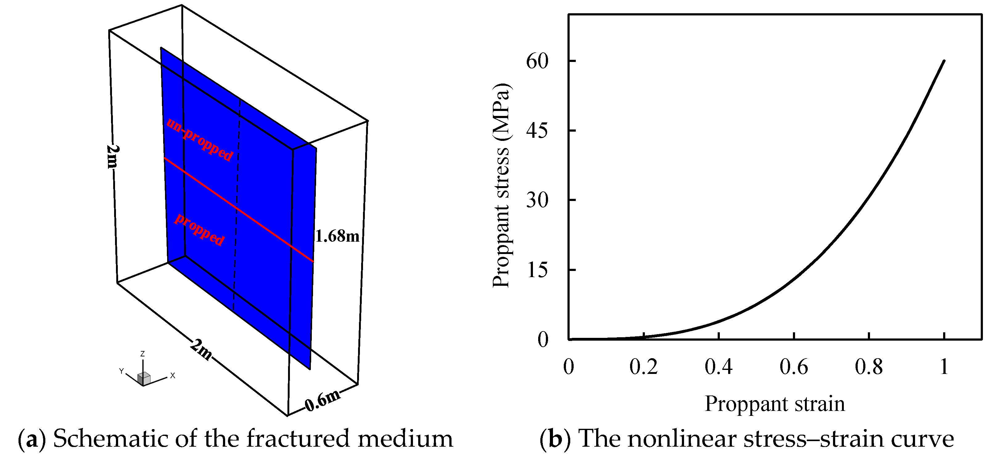
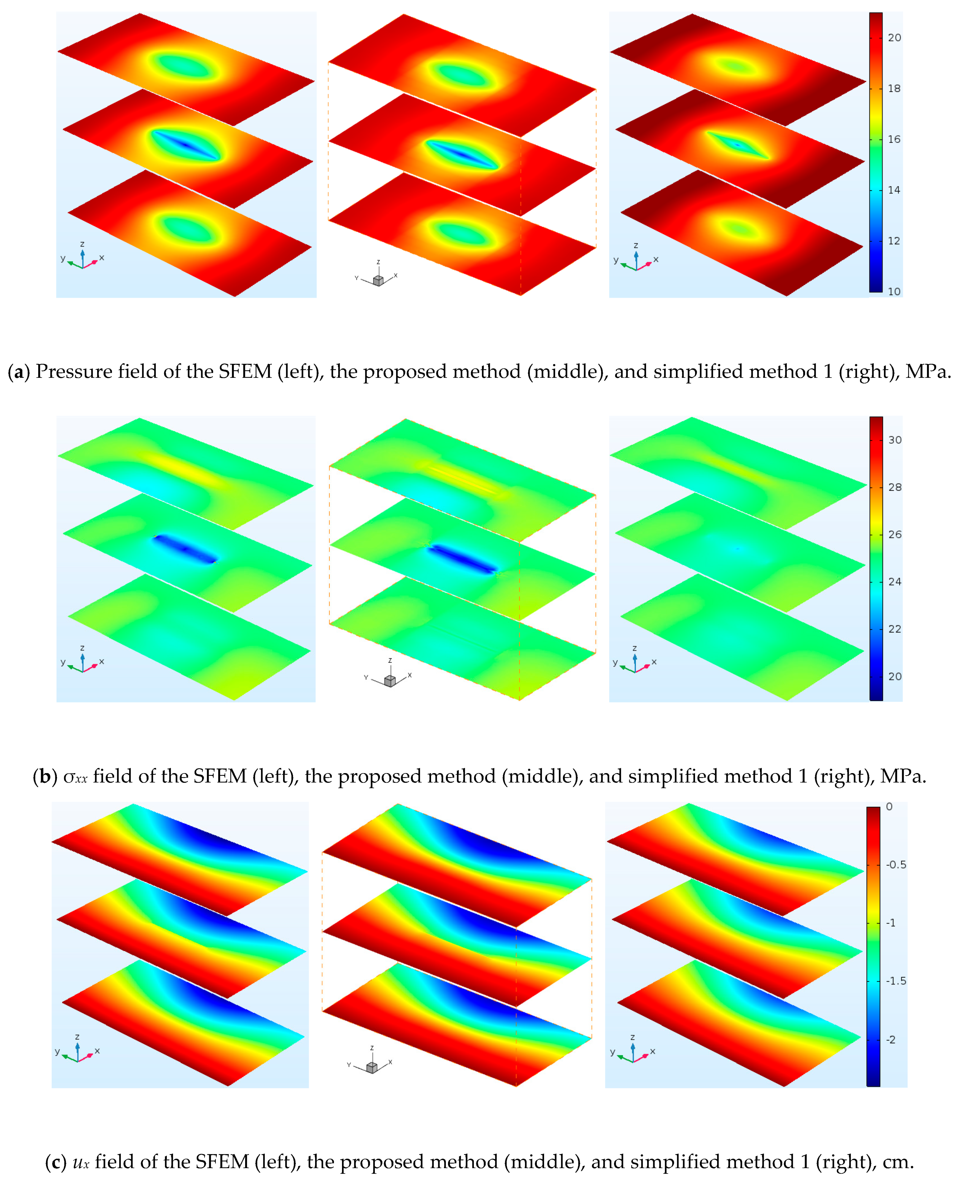
4.1.1. Partially Propped Fracture Deformation Problem

The model used to test the stabilized XFEM (S-XFEM) formulation for partially propped fracture deformation is shown in Figure 4a. This medium is homogenous (Young’s modulus: 1 GPa, Poisson’s ratio: 0.2) and contains one vertical fracture (1.68 × 1.68 × 0.005 m). Only one-half of the fracture (below the red line) is filled with proppant, and the nonlinear stress–strain curve of proppant is shown in Figure 4b. A uniform vertical downward constant load (100 MPa) is applied on the top boundary, while other boundaries are fixed in their normal directions. A displacement observation line (black dotted line) is located at the middle of the fracture. In this model, we simulate pure mechanical deformation, and compare the results of different methods.

Computational grids of the SFEM are refined near the fracture, and its number is 56,190. On the other hand, uniform grids (15 × 25 × 25) are used for the S-XFEM. The x-displacements obtained from the SFEM and S-XFEM are shown in Figure 5, and it can be seen that they are qualitatively close. This is because the S-XFEM can accurately simulate a partially propped fracture closure without requiring highly refined grids. Besides, it also shows that the deformation of the upper half of the fracture (un-propped) is greater than that of the lower half (propped). The computational times for simulating this model used by the SFEM and the proposed method are 15 s and 10 s, respectively.

The residual fracture apertures of the whole fracture, obtained from the SFEM (black dots) and S-XFEM (surface), are shown in Figure 6, and the excellent agreement between these results can be seen. In addition, Figure 6 also gives the residual fracture apertures along the displacement observation line, which are obtained from different methods (i.e., SFEM, S-XFEM and conventional XFEM). We can see that the result of S-XFEM is in good agreement with that of SFEM, while there is some oscillation in the result from conventional XFEM, especially at the fracture boundary. This is caused by the deficiency in displacement approximation (i.e., it does not satisfy the discrete LBB condition) of the conventional XFEM.

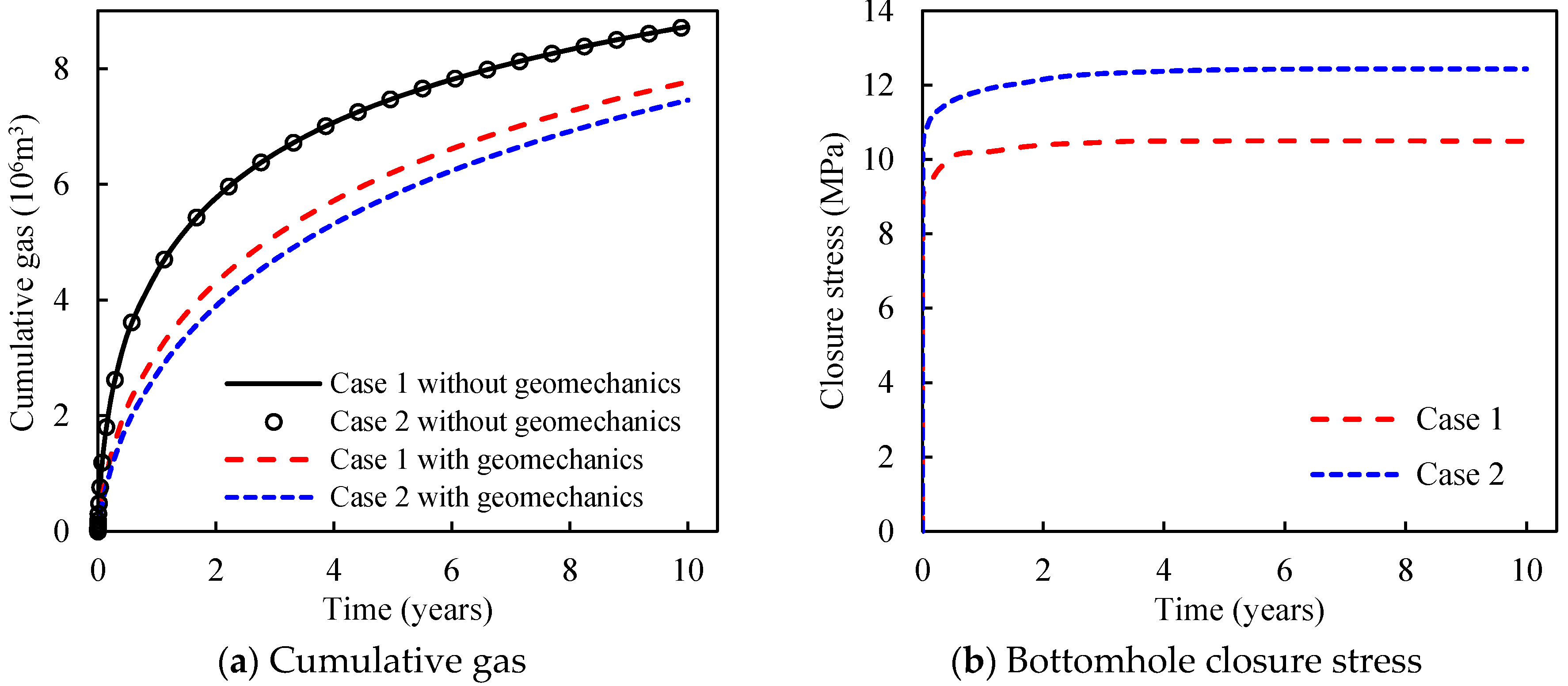
4.1.2. Gas Production and Stress Evolution in a 3D Fractured Shale Reservoir

As shown in Figure 7a, a 3D model is designed to validate the proposed method for predicting gas production and stress evolution in fractured shale reservoirs. A hydraulic fracture filled with proppant is at the center of this reservoir. For simplicity, this reservoir is assumed to be a dual-porosity and single-permeability medium, and the proppant deformation is assumed to be linear elastic. The production well is located at the center of the hydraulic fracture. For flow, we have no flow at the boundaries. For geomechanics, the uniform constant force (25 MPa) is applied on the top, right and back boundaries, and the other boundaries are fixed in their normal direction, respectively. The stress-dependent normalized fracture conductivity is shown in Figure 8, and other model properties are listed in

Table 1. Parameters of the shale reservoir for model verification.

Name	Value
Initial absolute permeability of matrix, m2	2 × 10−20
Initial absolute permeability of natural fracture, m2	1 × 10−17
Initial absolute permeability of hydraulic fracture, m2	1 × 10−17
Natural fracture spacing, m	1.0
Initial aperture of natural fracture and hydraulic fracture, m	5 × 10−6, 0.01
Initial porosity of matrix, natural fracture and hydraulic fracture	0.05, 1.0, 0.5
Young’s modulus of matrix, natural fracture and proppant, GPa	40.0, 40.0, 0.04
Poisson’s ratios of matrix and natural fracture	0.2, 0.2
Biot coefficient of matrix and natural fracture	1.0, 1.0
Langmuir pressure, MPa	4.0
Langmuir volume, m3/kg	0.018
Initial pressure and bottomhole pressure, MPa	25.0, 10.0
Reservoir temperature, K	343.15
Rock density, kg/m3	2850
Well radius, m	0.1

. Computational grids for the SFEM (169,082) and the proposed method (6417) are shown in Figure 7b,c, respectively.

Four different methods (i.e., SFEM, the proposed method, and the simplified methods 1 and 2) are applied to simulate the depletion production. The difference between the proposed method and simplified method 1 is that the displacement discontinuity at the hydraulic fracture was neglected in simplified method 1, while in simplified method 2, only the gas flow is simulated, and the geomechanical effects are simplified by correlating the fracture conductivity to pressure, which is based on the assumption that the total stress acting on the hydraulic fracture remains constant during depletion production. To make a better comparison of these methods, the permeabilities of the matrix and natural fractures are assumed to be constant.

The pressure, x-stress (σ_xx) and x-displacement (u_x) fields after 1000 days, obtained from different methods, are shown in Figure 9, and it can be seen that the results of the proposed method and SFEM are qualitatively close, while there are some differences between the results of simplified method 1 and SFEM, especially near the hydraulic fracture in the x-stress field, and this is caused by the neglect of displacement discontinuity. The computational times used by the SFEM and the proposed method are 220 s and 95 s, respectively. It can also be seen that the computational performance of the proposed method is better than that of the SFEM.

Comparisons of the cumulative gas and the evolution of σ_xx at the observation point (100, 215, 30) located on the hydraulic fracture are plotted in Figure 10. They show that the cumulative gas of simplified method 2 is significantly lower than that of the reference. This is because simplified method 2 overestimates the total stress acting on the hydraulic fracture, as shown in Figure 10b. The results of simplified method 1 show certain improvements, but there are still some differences compared with the references because of its neglect of displacement discontinuity. On the other hand, the results of the proposed method are almost the same as those of the references (the average errors of cumulative gas and the evolution of σ_xx are 2.26% and 0.5%, respectively). Therefore, the geomechanical and displacement discontinuity have significant impacts on gas production in shale reservoirs, and the proposed method can accurately simulate their effects.

4.2. Applications and Discussions

In this section, a series of case studies is conducted to study the effect of partially propped fracture closure on gas production in shale reservoirs. In order to reduce the simulation time, only one single stage (120 × 250 × 30 m) of a multi-stage hydraulic fractured shale reservoir is modeled, as shown in Figure 11a. The size of the SRV region (red dashed line) in this stage is 80 × 200 × 20 m, and the half-length and height of the hydraulic fracture are 90 m and 20 m, respectively. The production well is located at the center of the hydraulic fracture. For flow, we have no flow at the reservoir boundaries. For geomechanics, the overburden stress (30 MPa) is applied on the top boundary, two horizontal stresses (35 MPa, 40 MPa) are applied on the right and back boundaries, and the other boundaries are fixed in their normal directions, respectively. The model parameters are provided in

Table 2. Parameters of the shale reservoir for applications and discussions.

Name	Value
Initial absolute permeability of matrix, m2	2 × 10−20
Initial absolute permeability of natural fracture, m2	1 × 10−17
Initial absolute permeability of hydraulic fracture, m2	1 × 10−11
Natural fracture spacing and initial aperture of natural fracture, m	1.0, 5 × 10−6
Initial porosity of matrix, natural fracture and hydraulic fracture	0.05, 1.0, 0.5
Volume fraction of matrix sub-gridblocks	0.15, 0.21, 0.38, 0.26
Young’s modulus of matrix and natural fracture, GPa	40.0, 0.05
Poisson’s ratios of matrix and natural fracture	0.2, 0.2
Intrinsic solid grain bulk modulus, GPa	400.0
Langmuir pressure, MPa	4.0
Langmuir volume, m3/kg	0.018
Initial pressure and bottomhole pressure, MPa	25.0, 10.0
Reservoir temperature, K	343.15
Rock density, kg/m3	2850
Well radius, m	0.1

. The stress-dependent normalized fracture conductivity is shown in Figure 8, and the nonlinear stress–strain curve of proppant deformation is shown in Figure 12. Unless otherwise noted, these parameters and stress–strain curve are used for the following simulations. The dynamic permeabilities of the matrix, natural fracture and hydraulic fracture are calculated by using Equations (14)–(17). The computational grids used for this model are shown in Figure 11b. Please note that the surrounding rock (impermeable) is simulated for the better consideration of geomechanical effects in this model. For convenience, only the reservoir part is plotted in the following analysis.

4.2.1. Effect of initial Aperture Distribution

We first study the effect of initial aperture distribution on gas production through the following two different cases, as shown in Figure 13: (a) Case 1 with a more realistic aperture distribution obtained from geomechanical calculation, in which the initial pressure inside the hydraulic fracture is set as 42 MPa to mimic the fracturing process; (b) Case 2 with a uniform aperture of 0.005 m, which means Case 2 has the same cumulative gas as Case 1 when the geomechanical effect is not considered. Figure 14 illustrates the comparison of σ_xx distribution between Case 1 and Case 2 after 10 years. The results of cumulative gas and bottomhole closure stress are provided in Figure 15. We can see that the cumulative gas of Case 2 is slightly lower than that of Case 1. This is because that the aperture distribution has some effects on the total stress around the hydraulic fracture, and this results in a higher closure stress (acting on the hydraulic fracture) in Case 2, as shown in Figure 15b. Because the initial aperture distribution in Case 1 is more realistic than that in Case 2, it will be used in the following simulations.

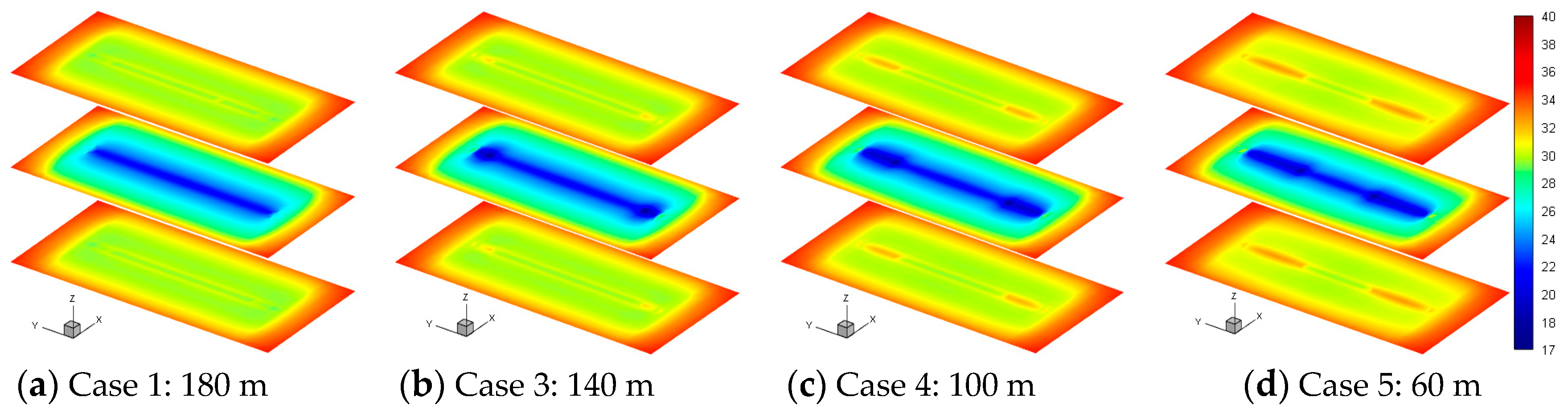
4.2.2. Effect of Propped Fracture Length

As shown in Figure 16, three cases, with propped fracture lengths of 140 m (Case 3), 100m (Case 4) and 60 m (Case 5), along with Case 1 (180 m), are used to investigate the effect of propped fracture length on gas production. Figure 17 illustrates the comparison of σ_xx distribution among the four cases after 10 years of depletion. We can see that the σ_xx around the propped fracture is slightly higher than that around the unpropped fracture. This is because the propped fracture part is stiffer than the unpropped part, which must suffer higher stress to support the boundary force. Figure 18 shows the comparisons of cumulative gas and production rate among the different cases. It can be seen that gas production correlates positively with the propped fracture length because of the increase in the contact area between the high-conductivity propped fracture and the matrix. Therefore, the completion design should strive to increase the length of the propped fracture so as to produce more gas.

4.2.3. Effect of Propped Fracture Height

To analyze the effect of propped fracture height on gas production, four cases with different propped fracture heights (Case 6: 15 m, Case 7: 10.5 m, Case 8: 9.5 m and Case 9: 5 m) are designed, as shown in Figure 19. It should be noted that the wellbore is placed on the propped fracture in Case 6 and Case 7, but on the unpropped fracture in Case 8 and Case 9.

The comparisons of σ_xx distribution and conductivity distribution among different cases after 10 years are illustrated in Figure 20 and Figure 21, respectively. The results of cumulative gas and production rate for different cases are provided in Figure 22. We can see that in Case 6, Case 7 and Case 9, gas production correlates positively with the propped fracture height. However, there is little difference between the gas production of Case 6 and Case 7, because the wells of both cases are located on the propped part of the hydraulic fracture, which leads to a large well production index. However, the gas production of Case 9 is much lower than that of Case 6 and Case 7 because of the limited conductivity of the unpropped fracture where the wellbore is located. Another interesting observation is that although the propped fracture height of Case 8 is less than that of Case 6 and Case 7, the gas production of Case 8 is higher. This is because the wellbore of Case 8 is placed on a high conductivity arch, which is usually formed at the top of the proppant bank, as shown in Figure 21. The fracture at this area may remain open throughout the production, which leads to an extremely large well production index.

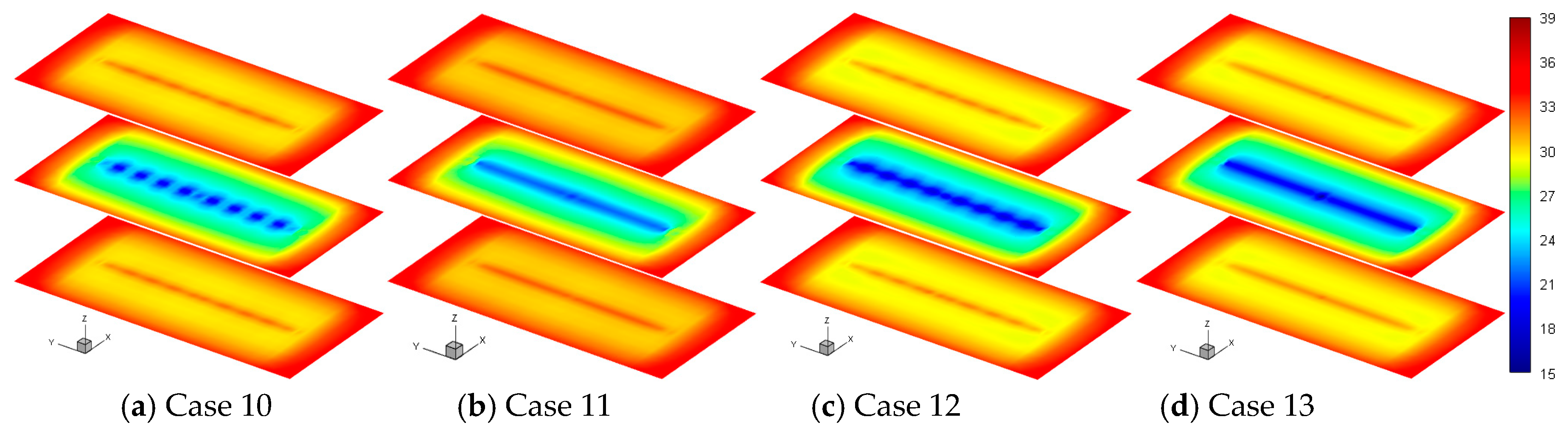
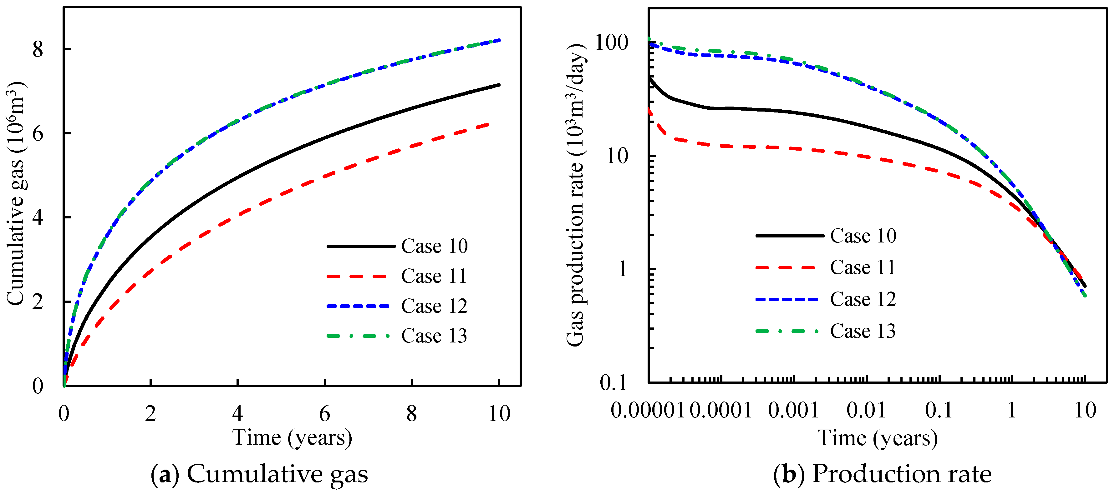
4.2.4. Effect of Proppant Distribution

Recently, the alternating (i.e., pulsed) injection of proppant-free fluids and proppant-containing fluids has been used to form heterogeneous proppant distributions (i.e., proppant pillars) [56,57]. The proppant pillars may withstand the closure stress to prevent the unpropped fracture between them being closed, and highly conductive flow channels can be generated. As shown in Figure 23, four cases (Cases 10–13) with different proppant distribution patterns are constructed to analyze the effects of proppant distribution on gas production.

The comparisons of σ_xx distribution and conductivity distribution among different cases after 10 years are illustrated in Figure 24 and Figure 25, respectively. We can see that in the first two cases, the highly conductive flow channels between proppant pillars are not connected, while they are connected in the other two cases. The results of cumulative gas and production rate for different cases are provided in Figure 26. It can be seen from the results of Case 10 and Case 11 that cumulative gas decreases as the number of flow channels increases. This is because gas flow in the fracture is mainly controlled by proppant pillars when the flow channels are not connected. The proppant pillars will withstand more closure stress as the flow channels increase, leading to the lower conductivity of the proppant pillars. Compared with Case 10 and Case 11, the cumulative gas is much higher in Case 12 and Case 13. However, the gas production curves are nearly overlapped for Case 12 and Case 13. This is because when flow channels are connected, the gas flow in the fracture is mainly controlled by the flow channels, and the fracture can be regarded as infinitely conductive in this situation. Therefore, improving the connectivity between flow channels is more important than increasing the number of flow channels.

5. Conclusions

The main contribution of this study is that we developed an efficient hybrid model, which includes the effect of each hydraulic fracture explicitly, with non-matching grids, and represents the effect of natural fractures implicitly, to simulate the closure of partially propped fractures and to examine the effect of this on gas production in fractured shale reservoirs. Besides, a stabilized XFEM iterative formulation based on the PPP technique is developed to accurately simulate a partially propped fracture closure with consideration of displacement discontinuity at fracture interfaces, and the modified fixed-stress sequential implicit method is applied to solve the coupled problem. We have validated our proposed method with the SFEM through some numerical examples, and the following conclusions are obtained from the case studies:

• The displacement discontinuity at hydraulic fractures and the initial aperture distribution of the hydraulic fractures have significant impacts on the evolution of stress near hydraulic fractures, thus a good performance can be predicted more accurately when these effects are considered;
• Gas production is positively correlated with the propped fracture length and height, and the connectivity between the well bore and the high conductivity arch plays an important role in production;
• Proppant distribution can significantly affect well performance. A fracture with alternating propped–unpropped–propped sections is favored because the highly conductive flow channels can be generated. In this fracture, improving the connectivity between flow channels is more important than increasing the number of flow channels.

References

1. Zhu, G.; Yao, J.; Sun, H.; Zhang, M.; Xie, M.; Sun, Z.; Lu, T. The numerical simulation of thermal recovery based on hydraulic fracture heating technology in shale gas reservoir. J. Nat. Gas Sci. Eng. 2016, 28, 305–316. [Google Scholar] [CrossRef]
2. Sakmar, S.L. The global shale gas initiative: Will the United States be the role model for the development of shale gas around the world. Hous. J. Int’l. L. 2010, 33, 369. [Google Scholar]
3. Yan, X.; Huang, Z.; Yao, J.; Li, Y.; Fan, D.; Sun, H.; Zhang, K. An efficient numerical hybrid model for multiphase flow in deformable fractured-shale reservoirs. SPE J. 2018, 23, 411–412,437. [Google Scholar] [CrossRef]
4. Giger, F.; Reiss, L.; Jourdan, A. The reservoir engineering aspects of horizontal drilling. In Proceedings of the SPE Annual Technical Conference and Exhibition, Houston, TX, USA, 16–19 September 1984; Society of Petroleum Engineers: Houston, TX, USA, 1984. [Google Scholar] [CrossRef]
5. Zeng, Q.; Yao, J.; Shao, J. Numerical study of hydraulic fracture propagation accounting for rock anisotropy. J. Pet. Sci. Eng. 2018, 160, 422–432. [Google Scholar] [CrossRef]
6. Zeng, Q.; Yao, J.; Shao, J. Study of hydraulic fracturing in an anisotropic poroelastic medium via a hybrid EDFM-XFEM approach. Comput. Geotech. 2019, 105, 51–68. [Google Scholar] [CrossRef]
7. Hubbert, M.K.; Willis, D.G. Mechanics of hydraulic fracturing. Mem. Am. Assoc. Pet. Geol. 1972, 18, 153–163. [Google Scholar] [CrossRef]
8. Memon, K.R.; Mahesar, A.A.; Ali, M.; Tunio, A.H.; Mohanty, U.S.; Akhondzadeh, H.; Awan, F.U.R.; Iglauer, S.; Keshavarz, A. Influence of Cryogenic Liquid Nitrogen on Petro-Physical Characteristics of Mancos Shale: An Experimental Investigation. Energy Fuels 2020, 34, 2160–2168. [Google Scholar] [CrossRef]
9. Mahesar, A.A.; Shar, A.M.; Ali, M.; Tunio, A.H.; Uqailli, M.A.; Mohanty, U.S.; Akhondzadeh, H.; Iglauer, S.; Keshavarz, A. Morphological and petro physical estimation of eocene tight carbonate formation cracking by cryogenic liquid nitrogen; a case study of Lower Indus basin, Pakistan. J. Pet. Sci. Eng. 2020, 192, 107318. [Google Scholar] [CrossRef]
10. Akhondzadeh, H.; Keshavarz, A.; Al-Yaseri, A.Z.; Ali, M.; Awan, F.U.R.; Wang, X.; Yang, Y.; Iglauer, S.; Lebedev, M. Pore-scale analysis of coal cleat network evolution through liquid nitrogen treatment: A Micro-Computed Tomography investigation. Int. J. Coal Geol. 2020, 219, 103370. [Google Scholar] [CrossRef]
11. Chen, Z.; Lin, M.; Wang, S.; Chen, S.; Cheng, L. Impact of un-propped fracture conductivity on produced gas huff-n-puff performance in Montney liquid rich tight reservoirs. J. Pet. Sci. Eng. 2019, 181, 106234. [Google Scholar] [CrossRef]
12. Lee, T.; Park, D.; Shin, C.; Jeong, D.; Choe, J. Efficient production estimation for a hydraulic fractured well considering fracture closure and proppant placement effects. Energy Explor. Exploit. 2016, 34, 643–658. [Google Scholar] [CrossRef]
13. Awan, F.U.R.; Keshavarz, A.; Akhondzadeh, H.; Al-Anssari, S.; Al-Yaseri, A.; Nosrati, A.; Ali, M.; Iglauer, S. Stable Dispersion of Coal Fines during Hydraulic Fracturing Flowback in Coal Seam Gas Reservoirs—An Experimental Study. Energy Fuels 2020, 34, 5566–5577. [Google Scholar] [CrossRef]
14. Liu, Y.; Leung, J.Y.; Chalaturnyk, R. Geomechanical simulation of partially propped fracture closure and its implication for water flowback and gas production. SPE Reserv. Eval. Eng. 2018, 21, 273–290. [Google Scholar] [CrossRef]
15. Zhou, L.; Shen, Z.; Wang, J.; Li, H.; Lu, Y. Numerical investigating the effect of nonuniform proppant distribution and unpropped fractures on well performance in a tight reservoir. J. Pet. Sci. Eng. 2019, 177, 634–649. [Google Scholar] [CrossRef]
16. Wang, J.; Elsworth, D. Role of proppant distribution on the evolution of hydraulic fracture conductivity. J. Pet. Sci. Eng. 2018, 166, 249–262. [Google Scholar] [CrossRef]
17. Liu, L.; Liu, Y.; Yao, J.; Huang, Z. Efficient Coupled Multiphase-Flow and Geomechanics Modeling of Well Performance and Stress Evolution in Shale-Gas Reservoirs Considering Dynamic Fracture Properties. SPE J. 2020, 25. [Google Scholar] [CrossRef]
18. Liu, Y.; Leung, J.Y.; Chalaturnyk, R.J.; Virues, C.J.J. New insights on mechanisms controlling fracturing-fluid distribution and their effects on well performance in shale-gas reservoirs. SPE Prod. Oper. 2019, 34, 564–585. [Google Scholar] [CrossRef]
19. Cipolla, C.L.; Warpinski, N.R.; Mayerhofer, M.; Lolon, E.P.; Vincent, M. The relationship between fracture complexity, reservoir properties, and fracture-treatment design. SPE Prod. Oper. 2010, 25, 438–452. [Google Scholar] [CrossRef]
20. Cipolla, C.; Lolon, E.; Mayerhofer, M. The Effect of Proppant Distribution and Un-propped Fracture Con-ductivity on Well Performance in Unconventional Gas Reservoirs. SPE 2009, 119368. [Google Scholar]
21. Sierra, L.; Sahai, R.R.; Mayerhofer, M.J. Quantification of Proppant Distribution Effect on Well Productivity and Recovery Factor of Hydraulically Fractured Unconventional Reservoirs. In Proceedings of the SPE/CSUR Unconventional Resources Conference—Canada, Calgary, AB, Canada, 30 September–2 October 2014; Society of Petroleum Engineers: Houston, TX, USA, 2014. [Google Scholar] [CrossRef]
22. Yu, W.; Zhang, T.; Du, S.; Sepehrnoori, K. Numerical study of the effect of uneven proppant distribution between multiple fractures on shale gas well performance. Fuel 2015, 142, 189–198. [Google Scholar] [CrossRef]
23. Yu, W.; Sepehrnoori, K. Simulation of proppant distribution effect on well performance in shale gas reservoirs. In Proceedings of the SPE Unconventional Resources Conference Canada, Calgary, AB, Canada, 5–7 November 2013; Society of Petroleum Engineers: Houston, TX, USA, 2013. [Google Scholar] [CrossRef]
24. Zheng, S.; Kumar, A.; Gala, D.P.; Shrivastava, K.; Sharma, M.M. Simulating Production from Complex Fracture Networks: Impact of Geomechanics and Closure of Propped/Unpropped Fractures. In Proceedings of the Unconventional Resources Technology Conference, Denver, CO, USA, 22–24 July 2019; pp. 2322–2338. [Google Scholar]
25. Zheng, S.; Manchanda, R.; Sharma, M.M. Modeling Fracture Closure with Proppant Settling and Embedment during Shut-in and Production. SPE Drill. Completion 2020. [Google Scholar] [CrossRef]
26. Moinfar, A.; Varavei, A.; Sepehrnoori, K.; Johns, R. Development of a Novel and Computationally-Efficient Discrete-Fracture Model to Study IOR Processes in Naturally Fractured Reservoirs. In Proceedings of the SPE Improved Oil Recovery Symposium, Tulsa, OK, USA, 14–18 April 2012; Society of Petroleum Engineers: Houston, TX, USA, 2012. [Google Scholar] [CrossRef]
27. Yan, X.; Huang, Z.; Yao, J.; Li, Y.; Fan, D. An efficient embedded discrete fracture model based on mimetic finite difference method. J. Pet. Sci. Eng. 2016, 145, 11–21. [Google Scholar] [CrossRef]
28. Yan, X.; Huang, Z.; Yao, J.; Li, Y.; Fan, D.; Zhang, K. An efficient hydro-mechanical model for coupled multi-porosity and discrete fracture porous media. Comput. Mech. 2018, 62, 943–962. [Google Scholar] [CrossRef]
29. Bochev, P.B.; Dohrmann, C.R.; Gunzburger, M.D. Stabilization of Low-order Mixed Finite Elements for the Stokes Equations. Siam J. Numer. Anal. 2004, 44, 82–101. [Google Scholar] [CrossRef]
30. Liu, F.; Borja, R.I. Stabilized low-order finite elements for frictional contact with the extended finite element method. Comput. Methods Appl. Mech. Eng. 2010, 199, 2456–2471. [Google Scholar] [CrossRef]
31. White, J.A.; Borja, R.I. Stabilized low-order finite elements for coupled solid-deformation/fluid-diffusion and their application to fault zone transients. Comput. Methods Appl. Mech. Eng. 2008, 197, 4353–4366. [Google Scholar] [CrossRef]
32. Kim, J.; Sonnenthal, E.L.; Rutqvist, J. Formulation and sequential numerical algorithms of coupled fluid/heat flow and geomechanics for multiple porosity materials. Int. J. Numer. Methods Eng. 2012, 92, 425–456. [Google Scholar] [CrossRef]
33. Kim, J.; Tchelepi, H.A.; Juanes, R. Stability and convergence of sequential methods for coupled flow and geomechanics: Fixed-stress and fixed-strain splits. Comput. Methods Appl. Mech. Eng. 2011, 200, 1591–1606. [Google Scholar] [CrossRef]
34. Versteeg, H.K.; Malalasekera, W. An Introduction to Computational Fluid Dynamics: The Finite Volume Method; Pearson Education: Glasgow, UK, 1995; p. 400. [Google Scholar]
35. Zhu, G.; Chen, H.; Yao, J.; Sun, S. Efficient energy-stable schemes for the hydrodynamics coupled phase-field model. Appl. Math. Model. 2019, 70, 82–108. [Google Scholar] [CrossRef]
36. Zhu, G.; Kou, J.; Yao, B.; Wu, Y.S.; Yao, J.; Sun, S. Thermodynamically consistent modelling of two-phase flows with moving contact line and soluble surfactants. J. Fluid Mech. 2019, 879, 327–359. [Google Scholar] [CrossRef]
37. Zhu, G.; Kou, J.; Yao, J.; Li, A.; Sun, S. A phase-field moving contact line model with soluble surfactants. J. Comput. Phys. 2020, 405, 109170. [Google Scholar] [CrossRef]
38. Wu, Y.-S.; Li, J.; Ding, D.; Wang, C.; Di, Y. A generalized framework model for the simulation of gas production in unconventional gas reservoirs. SPE J. 2014, 19, 845–857. [Google Scholar] [CrossRef]
39. Langmuir, I. The constitution and fundamental properties of solids and liquids. J. Frankl. Inst. 1917, 183, 102–105. [Google Scholar] [CrossRef]
40. Song, W.; Yao, J.; Li, Y.; Sun, H.; Zhang, L.; Yang, Y.; Zhao, J.; Sui, H. Apparent gas permeability in an organic-rich shale reservoir. Fuel 2016, 181, 973–984. [Google Scholar] [CrossRef]
41. Freeman, C.; Moridis, G.; Blasingame, T. A numerical study of microscale flow behavior in tight gas and shale gas reservoir systems. Transp. Porous Media 2011, 90, 253. [Google Scholar] [CrossRef]
42. Zhang, Q. Hydromechanical modeling of solid deformation and fluid flow in the transversely isotropic fissured rocks. Comput. Geotech. 2020, 128, 103812. [Google Scholar] [CrossRef]
43. Mohammadnejad, T.; Andrade, J. Numerical modeling of hydraulic fracture propagation, closure and reopening using XFEM with application to in-situ stress estimation. Int. J. Numer. Anal. Methods Geomech. 2016, 40, 2033–2060. [Google Scholar] [CrossRef]
44. Liu, J.; Chen, Z.; Elsworth, D.; Qu, H.; Chen, D. Interactions of multiple processes during CBM extraction: A critical review. Int. J. Coal Geol. 2011, 87, 175–189. [Google Scholar] [CrossRef]
45. Zhang, L.; Jing, W.; Yang, Y.; Yang, H.; Guo, Y.; Sun, H.; Zhao, J.; Yao, J. The investigation of permeability calculation using digital core simulation technology. Energies 2019, 12, 3273. [Google Scholar] [CrossRef]
46. Witherspoon, P.A.; Wang, J.S.; Iwai, K.; Gale, J. Validity of cubic law for fluid flow in a deformable rock fracture. Water Resour. Res. 1980, 16, 1016–1024. [Google Scholar] [CrossRef]
47. Shao, J.; Zhang, Q.; Sun, W.; Wang, Z.; Zhu, X. Numerical Simulation on Non-Darcy Flow in a Single Rock Fracture Domain Inverted by Digital Images. Geofluids 2020, 2020. [Google Scholar] [CrossRef]
48. Roostaei, M.; Nouri, A.; Fattahpour, V.; Chan, D. Coupled Hydraulic Fracture and Proppant Transport Simulation. Energies 2020, 13, 2822. [Google Scholar] [CrossRef]
49. Tan, Y.; Pan, Z.; Liu, J.; Wu, Y.; Haque, A.; Connell, L. Experimental study of permeability and its anisotropy for shale fracture supported with proppant. J. Nat. Gas Sci. Eng. 2017, 44, 250–264. [Google Scholar] [CrossRef]
50. Kim, J.; Seo, Y.; Wang, J.; Lee, Y. History Matching and Forecast of Shale Gas Production Considering Hydraulic Fracture Closure. Energies 2019, 12, 1634. [Google Scholar] [CrossRef]
51. Ghanizadeh, A.; Clarkson, C.; Deglint, H.; Vahedian, A.; Aquino, S.; Wood, J. Unpropped/propped fracture permeability and proppant embedment evaluation: A rigorous core-analysis/imaging methodology. In Proceedings of the Unconventional Resources Technology Conference, San Antonio, TX, USA, 1–3 August 2016; Society of Exploration Geophysicists, American Association of Petroleum: Tulsa, OK, USA, 2016; pp. 1824–1852. [Google Scholar] [CrossRef]
52. Li, X.; Feng, Z.; Han, G.; Elsworth, D.; Marone, C.; Saffer, D.; Cheon, D. Permeability evolution of propped artificial fractures in Green River shale. Rock Mech. Rock Eng. 2017, 50, 1473–1485. [Google Scholar] [CrossRef]
53. Tan, Y.; Pan, Z.; Liu, J.; Feng, X.; Connell, L. Laboratory study of proppant on shale fracture permeability and compressibility. Fuel 2018, 222, 83–97. [Google Scholar] [CrossRef]
54. Khoei, A.R. Extended Finite Element Method: Theory and Applications; John Wiley & Sons Inc.: West Sussex, UK, 2015; pp. 1–565. [Google Scholar]
55. Multiphysics, C. Introduction to COMSOL Multiphysics; COMSOL Multiphysics: Burlington, MA, USA, 1998; Volume 9, p. 2018. [Google Scholar]
56. Yan, X.; Huang, Z.; Yao, J.; Song, W.; Li, Y.; Gong, L. Theoretical analysis of fracture conductivity created by the channel fracturing technique. J. Nat. Gas Sci. Eng. 2016, 31, 320–330. [Google Scholar] [CrossRef]
57. Medvedev, A.V.; Kraemer, C.C.; Pena, A.A.; Panga, M.K.R. On the mechanisms of channel fracturing. In Proceedings of the SPE Hydraulic Fracturing Technology Conference, The Woodlands, TX, USA, 4–6 February 2013; Society of Petroleum Engineers: Houston, TX, USA, 2013. [Google Scholar] [CrossRef]
Figure 1. Schematic of a shale gas reservoir after hydraulic fracturing.
Energies 13 05339 g001
Figure 2. Sketch of a fractured porous medium and its boundaries.
Energies 13 05339 g002
Figure 3. Schematic of the fixed stress sequential implicit method.
Energies 13 05339 g003
Figure 4. Schematic of a 3D fractured medium and the nonlinear stress–strain curve.
Energies 13 05339 g004
Figure 5. Comparison of x-displacement obtained from two different methods, mm.
Energies 13 05339 g005
Figure 6. Comparisons of the residual fracture apertures of whole fracture and the residual fracture apertures along the displacement observation line.
Energies 13 05339 g006
Figure 7. Schematic of reservoir model and the computational grids for two different methods.
Energies 13 05339 g007
Figure 8. Normalized fracture conductivity under different closure stress, modified from Liu et al. (2018) [14].
Energies 13 05339 g008
Figure 9. Comparisons of pressure, x-stress and x-displacement for different methods after 1000 days. The profiles are shown in the top, middle and bottom layers, and the length in the z-direction is shown at five times the real size.
Energies 13 05339 g009
Figure 10. Comparisons of cumulative gas and observation point total stress obtained from different methods.
Energies 13 05339 g010
Figure 11. Schematic of the reservoir model and its computational grids.
Energies 13 05339 g011
Figure 12. The nonlinear stress–strain curve of proppant deformation, modified from Liu et al. (2018) [14].
Energies 13 05339 g012
Figure 13. Comparison of the aperture distribution: (a) Case 1, (b) Case 2.
Energies 13 05339 g013
Figure 14. Comparison of σxx distribution between Case 1 and Case 2 after 10 years, MPa. The profiles are shown in the top, middle and bottom layers, and the length in the z-direction is shown at 6.67 times the real size.
Energies 13 05339 g014
Figure 15. Comparisons of cumulative gas and bottomhole closure stress obtained form Case 1 and Case 2.
Energies 13 05339 g015
Figure 16. Four fracture profiles with different lengths of propped fracture (gray: propped; white: unpropped).
Energies 13 05339 g016
Figure 17. Comparison of σxx distribution between different cases after 10 years, MPa. The profiles are shown in the top, middle and bottom layers, and the length in the z-direction is shown as 6.67 times the real size.
Energies 13 05339 g017
Figure 18. Comparisons of cumulative gas and production rate obtained from different cases.
Energies 13 05339 g018
Figure 19. Four fracture profiles with different propped fracture heights (gray: propped; white: unpropped).
Energies 13 05339 g019
Figure 20. Comparison of σxx distribution between different cases after 10 years, MPa. The profiles are shown in the top, middle and bottom layers, and the length in the z-direction is shown as 6.67 times the real size.
Energies 13 05339 g020
Figure 21. Comparison of conductivity distribution between different cases after 10 years, lg(kHF·dHF/md-m).
Energies 13 05339 g021
Figure 22. Comparisons of cumulative gas and production rate obtained from different cases.
Energies 13 05339 g022
Figure 23. Four fracture profiles with different proppant distributions (gray: propped; white: unpropped).
Energies 13 05339 g023
Figure 24. Comparison of σxx distribution between different cases after 10 years, MPa. The profiles are shown in the top, middle and bottom layers, and the length in the z-direction is shown as 6.67 times the real size.
Energies 13 05339 g024
Figure 25. Comparison of conductivity distribution between different cases after 10 years, lg(kHF·dHF/md-m).
Energies 13 05339 g025
Figure 26. Comparisons of cumulative gas and production rate obtained from different cases.
Energies 13 05339 g026