Abstract
The article examines the relationship between CO2 equivalent emissions and agricultural production, taking into account additional economic and social variables that correct the considered relationship for the six Central and Eastern European countries over the period 1992–2017. The aim of the article was to confirm or negate the occurrence of the environmental Kuznets curve (EKC) in the countries of Central and Eastern Europe. Countries that experienced a political transformation and were subsequently admitted to the European Union (EU) undergoing a preparatory period were included. The topic is timely as all EU countries are required to monitor their emissions under the EU Climate Monitoring Mechanism. The discussed problem is significant due to the changes taking place in the common agricultural policy, the choice of actions to be taken by individual countries in their national policies, and the choice of instruments to support the transformation of agriculture. Agriculture has a particularly large impact on emissions, especially N2O and CH4. This paper uses GLS (Generalized least squares) panel regression with random effects taking into consideration individual effects for countries. The conducted empirical research confirmed the hypothesis regarding the occurrence of the Kuznets curve in relation to agricultural production. In this situation, it is required to increase the activities of maintaining production growth, with the support of technological changes that significantly increase pro-environmental conditions, because, in the current circumstances, this growth takes place with an increase in CO2 gas emissions, thus leading to negative external effects.
1. Introduction
Research conducted for a long time on the impact of different factors on the volume of greenhouse gas emissions with an attempt to explain the relationship between the volume of emissions and the rate of economic growth, as well as production and consumption, carried out in different spatial and temporal cross-sections, indicated the occurrence of heterogeneous relationships. However, many interesting guidelines were provided for national policies and the determinants of these processes in individual countries and regions. These relations can be considered on the basis of the Kuznets curve, indicating at what stage of transformation a particular economy or the market under consideration is, as originally presented by J. Kraft and A. Kraft [1]. As it results from the statistical data presented in this study (Table 1), the assessment problem results from the large diversity between individual countries and markets; therefore, it seems reasonable to conduct such an assessment in relation to individual groups of countries or markets with similar social, economic, and political conditions. Taking these guidelines into account, a reference is made to changes in the common agricultural policy affecting the relationship between CO2 equivalent emissions and agricultural production in the countries of Central and Eastern Europe that are European Union (EU) members. This is due to the ongoing debate on the shape of this policy in upcoming budgets. The need for a sectoral approach has often been pointed out in the literature due to the different transformations and relationships between changes in production volumes and greenhouse gas emissions [2].

Table 1.
CO2 emission in the countries of Central and Eastern Europe in 1992–2016.
When addressing the problem of relationships between the level of CO2 equivalent emissions and agricultural production and its conditions, attention should be paid to regional differences. Therefore, in this study, the research was conducted on a group of countries of Central and Eastern Europe that underwent the process of political transformation and were then subjected to the mechanism of a common agricultural policy. They experienced similar transformations of external factors and are also characterized by similar economic structures and a similar level of economic development. According to the concept presented by Shahbaz and Sinha [3], countries of this group at the level of the entire economy should show a relationship between greenhouse gas emissions and economic growth in line with the environmental Kuznets curve (EKC). In narrower terms, in relation to agricultural production, the existence of such a relationship for these countries does not seem so obvious, although, thanks to the financial support resulting from the mechanism of the Common Agricultural Policy (CAP) and earlier pre-accession funds, there were changes in the structure and technology of production in agriculture. Operation under the CAP requires that more and more pro-environmental requirements be met [4,5,6] to reduce negative externalities and to reduce CO2 equivalent emissions. For agricultural producers from Central and Eastern Europe, this is often a serious economic barrier due to the need to make significant investments, overcome legal and institutional restrictions, and increase production costs [7,8,9], as a result of disproportions in the level of the mentioned financial support [10] between individual EU countries. It also results from the low level of profitability of agricultural production and its significant changes in individual years (high risk of activity, high risk of operations) [11]. This is not a chronic problem, especially in the countries of the old European Union (EU-15), but it should be remembered that the level of income of agricultural producers was still supported by the financial support system [12]. It should also be noted that agriculture is not only an emitter of greenhouse gases, but also a complex system that captures some of the gas emissions in plant production, especially CO2 equivalent from the air [13,14]. Therefore, with an appropriate structure of crops, agriculture may play a role that limits its occurrence in the environment. Sequestration of additional carbon in the soil would reduce CO2 equivalent emissions to the atmosphere, thus mitigating global warming and improving soil fertility in agricultural applications. In this situation, the change in production technology in agriculture, stimulated by institutional factors, can not only contribute to a direct reduction in CO2 equivalent emissions, but also reduce the level of greenhouse gases emitted by other sectors of the economy. This approach creates a global public good, which nevertheless requires the creation of a specific financing system.
The problem of the relationship between the level of greenhouse gas emissions and the increase in production or income can be considered at the level of entire countries or for individual products. One of the special areas worth analyzing is agricultural production. This is due to several reasons. Research shows that agriculture makes a significant contribution to greenhouse gas emissions [15,16]. On the one hand, this is due to the significant share of agricultural production in global greenhouse gas emissions, estimated at 24% in 2014 (particularly with regard to nitrous oxide (N2O) and methane (CH4) emissions). The share of agriculture was estimated at 60% for N2O and 50% for CH4 on a global scale [17], whereas N2O emissions are particularly dangerous for the environment, because its greenhouse effect is about 310 times greater than CO2 equivalent emissions [18]. Moreover, an increasing trend in CO2 equivalent emission in agricultural production is still being maintained, although its pace is slowing down. In this context, it is worth noting that agricultural production in many countries is subject to complex agricultural policies, through which the conditions of doing business in this sector of the economy are regulated. These policies are increasingly focused on implementing technologies that reduce greenhouse gas emissions. A good example is the CAP and the introduction of even greening principles and earlier modulation.
The problem of greenhouse gas emissions and their effects, highlighted in the widely described topic of climate change in relation to agricultural production, also has a slightly different dimension [19,20,21,22,23]. As a result of the observed climate change, the impact of environmental conditions, which increases the global risk of economic activity in agriculture, is increasing, which affects the international competitive position and the reallocation of resources. Consequently, a significant decrease in the yield of basic agricultural crops is forecast in many regions [24,25]. Therefore, reducing emissions of these gases in the long run is beneficial for agriculture. As a result of ongoing climate change, high macroeconomic costs arise, limiting the possibilities of transferring funds to agriculture, as well as microeconomic costs, raising the costs of agricultural production.
This topic is timely as all EU countries are required to monitor their emissions under the EU Climate Monitoring Mechanism, which sets out internal EU reporting rules on the basis of internationally agreed commitments.
The reporting covers the following:
- emissions of seven greenhouse gases (the greenhouse gas inventory) from all sectors: energy, industrial processes, land use, land-use change, and forestry (LULUCF), waste, agriculture, etc., as well as projections, policies, and measures to cut greenhouse gas emissions;
- national measures to adapt to climate change;
- low-carbon development strategies;
- financial and technical support to developing countries, as well as similar commitments;
- national governmental use of revenues from the auctioning of allowances in the EU emissions trading system (committed to spending at least half of these revenues on climate measures in the EU and abroad).
There is a research gap in the presented area, resulting from the poor diagnosis of the situation in the studied group of countries (Table A1) and taking into account the ongoing structural changes in agriculture, influencing the conditions for greenhouse gas emissions. The scope of transformations in the selection of a group of countries was significant and resulted from their inclusion in the Common Agricultural Policy (CAP) [26]. Therefore, a change in the influence of external factors can be expected, which also prompted us to undertake research. Substantial research concerns the countries of Asia and Africa (Table A1). This is due to the relatively high share of agriculture in the creation of value added in these countries (the 5 year 2015–2019 average was 3.1%). However, in the examined Central and Eastern European countries, this share is also relatively large in relation to the EU-15 countries. On the other hand, research from other regions allows identifying potential factors influencing the relationship between gross domestic product (GDP) and gas emissions, as well as adequate research methods and conclusions for practical solutions resulting from them. The sectoral approach is also important due to the specificity of agricultural conditions and the applied agricultural policy (CAP).
The volume of CO2 equivalent emissions in the countries of Central and Eastern Europe that underwent political transformation after 1989 was relatively high, especially in the case of Poland (36,030.32 Gg of CO2 emissions in Poland). It resulted from the significant dependence of these economies on the production and processing of coal for the production of electricity. A similar situation was visible in agricultural production, where the increase in production intensity was due to the increase in intermediate consumption, often due to the use of chemicals. Despite the high greenhouse gas emissions, significant variation can be seen between the countries under consideration (Table 1, Figure 1a–f). Hungary, the Czech Republic, and Bulgaria had similar CO2 equivalent emissions. However, other countries showed different levels of emission patterns. This was mainly due to the slow transformation of these countries and the constantly high share of coal. At the beginning of the 1990s, the Slovaks emitted the least CO2, while Poles and Romanians emitted the most (Table 1, Figure 1a).
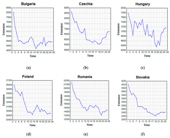
Figure 1.
CO2 emissions in agriculture in the countries of Central and Eastern Europe in 1992–2016: Bulgaria (a), Czechia (b), Hungary (c), Poland (d), Romania (e) and Slovakia (f). The variables on the x-axis represent the years of analysis (1992(0)–2016(26)). Source: own study according to FAOstat [27].
In the case of Poland, there was also a large range between the minimum and maximum values, and between the first and third quartiles. No outliers were observed here (as was the case with Romania or Bulgaria). The changes taking place in the economies during the period under review favored convergence mechanisms, in terms of both economic development and the amount of financial support for agriculture [28], which should translate into an approximation of CO2 equivalent emissions. Empirical results of the work of Strazicich and List [29] indicated that such convergence is possible.
The growing awareness of threats caused by the production of greenhouse gases, as well as the difficulties with selling agricultural products, forced changes in agricultural production technology and its structure. In all the analyzed countries there was a decrease in CO2 equivalent emission, which is consistent with the assumptions of the EKC hypothesis, as, at the same time, there was an increase in agricultural production (and GDP in agriculture (by 30.86% in 2000–2019—the average for the surveyed countries), although the sector’s share in the total GDP of the economy decreased from 5.78% to 2.89% in 2000–2019 (average for the analyzed countries). However, the dynamics of transformations, the level of fluctuations, and the direction of changes taking place in the last of the periods presented were different (Figure 1a–f). A particularly rapid decline in all countries occurred during the first 10 years of the analysis (1992–2001). This similarity allows the use of various econometric methods to determine the variability of occurring phenomena and describe them with a common model explaining these transformations. In the next subperiod, the changes were already multidirectional. Emissions increased in the Czech Republic and Hungary. Long-term permanent reduction took place only in Poland, while, in Bulgaria, Romania, and Slovakia in the last of the subperiods, there was a correction in the form of an increase in CO2 equivalent emission. The highest level of volatility occurred in Hungary, while, in Poland, despite a rapid decrease in emissions, its level remained the highest among the countries studied. The presented differences suggest the appearance of additional factors correcting the changes taking place, primarily of the nature of internal conditions, which are worth isolating and examining.
2. Literature Review
The growing interest in environmental pollution from an economic perspective is reflected in the environmental Kuznets curve. In its basic form, the Kuznets curve indicates the relationship between the level of GDP and the emission of pollutants into the environment. Its shape resembles an inverted U, and it can be formally written as follows [30]:
Today, many authors not only analyze the relationship of CO2 emissions to GDP, but also include a number of other variables. Marie-Noëlle [31] took into account the volume of exports and imports, the degree of openness of the economy, and private consumption and gross fixed capital formation in the analysis. Lindmark [32] also studied variables such as the fuel price index, technology level, and cement prices. Friedl and Getzner [33] studied via the regression equation additional variables such as the share of import and the share of the service sector. In turn, York [34] analyzed population size, age structure, economic development, and level of urbanization. A wide range of variables was also used by Lipinskiene, Tvaronaviciene, and Vaitkus [35] who considered value added in construction as a percentage of share in total value added in the economy, percentage of total taxes and social security contributions, ratio between energy tax revenues and final energy consumption (EUR per ton), research expenditure and experimental development (EUR), primary coal production and lignite (in tons), and ratio between gross domestic energy consumption and GDP (kg/EUR). In turn, Hnatyshyn [36], next to GDP per capita, analyzed the impact of foreign trade intensity and primary energy consumption. In many of the cited studies, an important factor increasing the level of greenhouse gas emissions was international exchange and the degree of openness of the economy [37,38,39]. This factor is one of the significant manifestations of globalization and better resource allocation in the global economy, which ambiguously affect the level of greenhouse gas emissions, depending on the approach. In light of the studies mentioned, the pro-export attitude and intensification of trade from the point of view of only CO2 equivalent emissions was unfavorable. To sum up the results so far, it should be stated that, in most studies, the Kuznets hypothesis was confirmed. On the other hand, it was denied, among others, in the works of Roca et al. [40] for Spain, Lindmark [32] for Sweden and Acaravci and Ozturk [41]. At the same time, critics of this approach indicate that an increase in income does not have to lead to an improvement in the environment [42]. The results obtained as a result of the analysis of the Kuznets curve have a significant impact on the formulation of domestic policy [40,43].
In the case of agriculture, research on the emissions of pollutants into the environment did not only include the analysis of the Kuznets hypothesis, but also the assessment of the emission itself without its relationship to an increase in production or GDP (Table 1). With regard to agricultural production, on the basis of the prepared statistics (Table 1), it can be stated that macroeconomic, microeconomic (sometimes associated with a particular type of agricultural production, e.g. cereals), social, environmental, or legal variables were taken into account. Repeated explanatory variables include (Table A1) GDP per capita, level of economic development, budget deficit, population size, fuel costs, energy consumption from various sources, biomass production volume, agricultural production prices, transport costs, gross value added from agriculture, coal consumption, fertilization level, afforestation level, urbanization rate, renewable energy production, innovations, agricultural production value, and agricultural subsidies. Such a wide spectrum of factors taken into account in the research indicates the complex nature of relationships and the important role of institutional and legal factors that are difficult to grasp, affecting the conditions in which agricultural production takes place. The research concerned all agriculture in a particular country or countries [44,45,46,47]; alternatively, it took a regional dimension [47,48] or specific agricultural market [49,50,51].
Numerous methods were used in studies on CO2 emission and the EKC hypothesis, primarily, regression and space–time analysis using various variables. Considerations carried out in relation to agriculture were similar to the general analysis, and the indicator method was often used to analyze the causes of changes in greenhouse gas emissions. An over view of agricultural research, with a detailed description of the methods used and the main results, is given in Table A1.
3. Materials and Methods
In this study, a period of 26 years (1992–2017) for six Central and Eastern European countries (Bulgaria, the Czech Republic, Hungary, Poland, Romania, and Slovakia) was used to analyze the relationship between CO2 equivalent emissions (expressed in Gg) and agricultural production. Countries that experienced a political transformation and were subsequently admitted to the EU undergoing a preparatory period were included. Thus, they underwent similar changes in external conditions and, at the same time, were characterized by a high level of CO2 equivalent emissions in the base period. The independent variables were included on the basis of the research to date (Table A1) and our own assessment. The selected variables were available in public statistics and related to the same periods for all analyzed countries. All variables are strongly related to greenhouse gas emissions from agriculture and have been used as explanatory variables in many studies (Table A1). They were represented by the total agricultural population (population total), the share of exports and imports of agricultural products in the gross agricultural product (XGPV), the gross production per capita index (2004–2006 = 100) (GPI), and the net production value in agriculture per capita (2004–2006 = 100; production value in constant values calculated on the basis of average prices for the selected year or years, known as the base period) (NPVpc). The relationship shown with the use of the Kuznets curve is helpful in determining the applied economic policy, while the determination of the current position of the economy on the curve illustrates the degree of advancement of environmental economic processes that have occurred so far and indicates future prospects. An additional variable called square NPV (sqNPVpc) was created to determine the shape of the environmental Kuznets curve. All data came from the FAOstat database [27]. All variables were logged. The study used a panel analysis with fixed effects (FE) and random effects (RE). A common panel data regression model is shown in Equation (2), where y is the dependent variable x is the independent variable, α and β are coefficients, and i and t are indices for individuals and time. Error is very important in this analysis. Assumptions about the error term determine whether we speak of fixed effects or random effects. In a fixed effects model, it is assumed to vary non-stochastically, making the fixed effects model analogous to a dummy variable model in one dimension. In a random effects model, it is assumed to vary stochastically, requiring special treatment of the error variance matrix.
where vit is the total random error, which consists of the purely random part (Ɛit) and the individual effect ui(vit = Ɛit + ui).
After taking into account the considered variables, the model hypothesis for the panel took the following form:
where ui is the individual effect, and ei is the purely random error.
Annual data were used in the studies. The choice of the model form among independently pooled panels, fixed effects model (FE), and random effects model (RE) was made on the basis of the Hausman test. The obtained result (Prob > chi2 = 0.0499) indicated the use of the FE model, although this value was at the borderline level. Therefore, in the adopted study, both FE and RE models were estimated. The β estimator in the random model takes the following form:
where X is the matrix of the explanatory variables, y is the vector of the dependent variables, and Ω is the variance and covariance matrix of the total random error. The matrix Ω takes the following form:
where
4. Results and Discussion
The FE model panel data provide the ability to control unobservable variables that change over time, but not between countries. In the case of the FE model, the relationship between the predictor and the output variables within the country was examined. The time-stable unobservable features in the FE model should not be correlated with other individual features. In the FE model, the influence of interactions unchanging in time was removed, which allowed for the assessment of the actual net effect of the analyzed predictors on the studied variable. In the case of the RE model, it was assumed that the variability between countries was random and uncorrelated with independent variables. The Hausman test (Figure 2) was used to select the analytical form of the model.
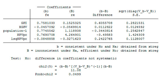
Figure 2.
Hausman test for the panel model. Source: Own calculations according to FAOstat data [27].
Standard diagnostics of the Hausman test indicated that, for values < 5%, an analysis of the model with random effects (RE) should be performed. The obtained result was on the border of the accepted limit value; therefore, both FE and RE models were performed (Figure 3 and Figure 4). In order to eliminate heteroscedasticity, the GLS (Generalized least squares) RE model was used, while, for the FE model, robust errors were used.
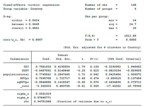
Figure 3.
CO2 model with fixed effects (FE). Source: Own calculations according to FAOstat data [27].
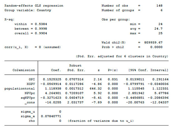
Figure 4.
CO2 model with random effects (RE). Source: Own calculations according to FAOstat data [27].
The low value of the F test indicated the correctness of the regression estimation, despite the lack of significance of some structural parameters in the FE model (Figure 3). In the analyzed case, almost 95% of the variance resulted from differences between the panels, and the ui errors were strongly correlated with the regressors. The analytical form confirmed the presence of the inverted Kuznets curve. In this case, the turning point was 4.53003 for net production value in agriculture per capita (2004–2006 = 100). The increase in production, measured by gross production per capita, increased the value of CO2 equivalent emissions; however, in terms of net production, there was a different form of dependence. A similar slope factor occurred in the case of the population, which is consistent with the results in other studies, including Lin and Xu [52], Xu and Lin [53], and Long, Lou, Wu and Zhang [54].
In the RE model, the slope factors followed the FE model. Wald’s test indicates the correctness of the model, and the differences between the units were not correlated with the regressors (Prob > chi2 = 0; Figure 4). All parameters in this model were statistically significant at a level lower than 0.05 (p < 0.05; Figure 4 and Figure 5). This indicates the presence of an inverted Kuznets curve at a turning point at the level of 6.5180 for production value in agriculture per capita. The direction of the impact of individual variables was the same as in the FE model (Figure 5). A low value of the coefficient in the sqNPVpc variable means a high level of “expropriation” of the relationship between agricultural production and CO2 equivalent emissions. Thus, in the present conditions, an increase in production would result in a less than proportional increase in CO2 equivalent emissions and even a decrease in the longer term. All the considered countries were on the left side of the curve; thus, the increase in net production was still accompanied by an increase in CO2 equivalent emissions, but they were close to the top of the function. Poland and Hungary were relatively the closest, but the differences were not significant. This also means that the transformations in the agricultural production system and the applied technology in these countries were very similar.
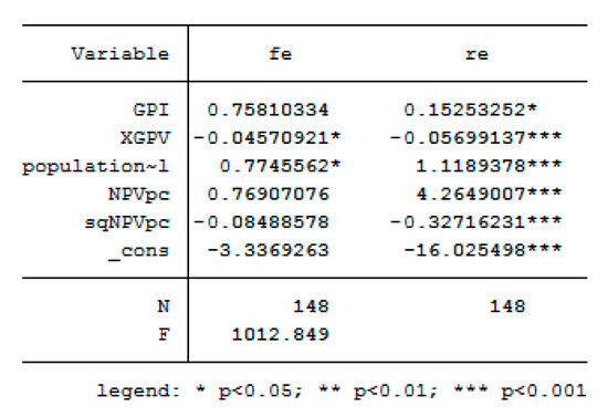
Figure 5.
Comparison of FE and RE models for CO2 emissions. Source: Own calculations according to FAOstat data [27].
The estimated parameters of the panel models with variable effects (RE) and fixed effects (FE) confirmed the presence of the environmental Kuznets curve in relation to agricultural production in the countries of Central and Eastern Europe. Most of the analyzed factors were positively related to CO2 equivalent emissions. The flexibility of the relationship for positively related variables was very similar (both for the population size and for net and gross agricultural production). As a consequence, there were effects of scale of operations for the provision of environmental services, resulting from technological changes and the substitution of labor with capital, allowing for an increase in production. Only the variable XGPV was diagnosed with a negative value. In this case, the level of flexibility was in absolute terms lower than the previous factors. The impact of the degree of openness on international exchange in the literature is not clear. This study showed that this degree in the case of agricultural products has a positive effect and reduces the level of pollution. This should be combined with increased competition leading to lower environmental costs. In the case of many countries, replacement requires meeting the growing phytosanitary and environmental requirements in terms of the conditions in which agricultural production takes place, which leads to the selection of techniques limiting the negative impact on the environment in the form of lower CO2 equivalent emissions. This applies in particular to the EU market, which is crucial for the studied countries. This effect does not apply to all entities; hence, the value of the coefficient is lower than others. In the analyzed case of the variance “within”, it was much lower than the variance “between”. This points to the fact that the developed model better explains the differences in emissions between countries than within countries, whereby changes in individual countries did not show such stagnant differences across individual years. The Rho value was equal to 0. Therefore, the conditions that remain unchanged in time and are not observable in the analyzed group of countries had a marginal impact on the value of the total random error, and the remaining part involved purely random variability. Therefore, the average levels of the independent variables for the entire period in individual countries were very similar. This confirmed the variation between countries. According to Kilic and Balan [55], the condition for the Kuznets curve to appear is that the structural parameters defining the trend function take the following form:
A negative value of the coefficient for sqNPVpc indicates that the parabola plot took the shape of an inverted U letter. Furthermore, the value of the estimated coefficient was low, with a higher standard error. At the present stage of transformation, along with the increase in production, agriculture may generate greater amounts of carbon dioxide. The presented results suggest that national policies aimed at limiting greenhouse gas emissions are a necessary tool in this group of countries. Despite the significant decrease in the amount of emissions from agriculture at the beginning of the considered period, the change in the value of net production did not offset changes in the volume of these emissions. Agriculture is a particular sector highly susceptible to fluctuations in environmental conditions in this climate, which makes it difficult to define its long-term growth model. The effect of gross production impact, including intermediate consumption, i.e., the purchase of raw materials and auxiliary materials, had a negative impact; however, it was related to a number of inputs influencing the intensity of production and generating the emission of pollutants into the environment (fertilizers, feed, or plant protection chemicals). Therefore, their high share, increasing the gross value of production, had a positive effect on the level of pollution.
Studies in developing countries have largely confirmed the presence of EKC (Table A1). They did not reach their peak and, as a result, the increase in agricultural production positively influenced the increase in CO2 emissions [18,47,50,52,53,56]. The mechanization of agriculture also increased greenhouse gas emissions. Only the experience of developed countries, the introduction of innovations, and the use of renewable energy in agricultural production to a greater extent changed this effect [18,54,57,58]. Thus, the solutions in the studied countries should, first of all, favor a greater possibility of implementing innovations and changes in the structure of energy consumption. The conducted research confirms the stated considerations and shows that the scope of the transformations increasingly enables the application of measures introducing a more restrictive approach to limiting the solutions increasing the emission of greenhouse gases. A further increase in agricultural production in these countries, in the light of the results obtained, indicates that anincrease in production is less related to additional greenhouse gas emissions.
5. Conclusions
This paper explored the relationship between CO2 equivalent emissions and agricultural production for the Central and Eastern European countries over the period 1992–2017. The conducted research confirmed the existence of a dependence in the form of the Kuznets curve in relation to the agricultural production of Central and Eastern European countries, despite the differences in the implemented CO2 emission reduction paths. This has significant implications for establishing a common agricultural policy, especially since there is a debate on its further shape in the upcoming financial perspectives. The found transformations in the production structure and the technologies used for its production show that it was possible to find a sustainable development path between the increase in agricultural production and CO2 equivalent emissions from agriculture. In the present conditions, it is increasingly justified to apply solutions increasing the role of pro-environmental factors limiting the level of greenhouse gas emissions. Increasing agricultural production places a lower burden on the natural environment in terms of greenhouse gas emissions. In the longer term, the opposite relationship should be expected, whereby an increase in production will not be positively related to an increase in CO2 equivalent emissions. In relation to these countries, an application of solutions corresponding to the current situation of individual countries is required in terms of agricultural production. This is particularly important due to the relatively high level of pollution emissions in the studied countries, including greenhouse gases. As a consequence, it is possible to increase production in agriculture with a low environmental cost and limitation of negative effects. This confirms the legitimacy of changes in the common agricultural policy aimed at increasing the principles of greening and increasing pro-environmental instruments, which is justified not only socially, but also economically for the countries of Central and Eastern Europe.
The presented situation, in line with the inverted U curve between the emission of greenhouse gases and the increase in agricultural production in the analyzed countries, requires the application of institutional solutions as part of the sectoral policy. It is necessary to introduce incentives for agricultural producers to use energy-saving and low-carbon technologies in agricultural production. It should be noted, however, that an increase in production has little effect on increasing CO2 equivalent emissions. Such solutions should facilitate, as well as co-finance, an investment in modern technologies or use agricultural technology that reduces emissions per product unit. Therefore, they require a constant modernization of agriculture in the researched countries, conditioned by environmental and social aspects. At the same time, it seems increasingly justified to tighten the standards in the field of greenhouse gas emissions, as it limits the growth of agricultural production to a lesser extent.
Author Contributions
Conceptualization, P.K.; methodology, P.K. and Ł.A.; software, P.K. and Ł.A.; validation, P.K. and Ł.A.; formal analysis, P.K. and Ł.A.; investigation, P.K. and Ł.A.; resources, P.K. and Ł.A.; data curation, P.K. and Ł.A.; writing—original draft preparation, P.K. and Ł.A.; writing—review and editing, P.K. and Ł.A.; visualization, P.K. and Ł.A.; supervision, P.K. and Ł.A.; project administration, P.K. and Ł.A. All authors have read and agreed to the published version of the manuscript.
Funding
This research received no external funding.
Conflicts of Interest
The authors declare no conflict of interest.
Appendix A
Table A1.
Emissions of pollutants into the environment through agriculture.
Table A1.
Emissions of pollutants into the environment through agriculture.
| Author | Analysis Period | Region | Agriculture Area | Method | Variables | Main Results |
|---|---|---|---|---|---|---|
| Li et al. (2016) [59] | 1995–2009 | 18 EU member states | All agriculture | Index decomposition analysis (IDA), facilitated by the Shapley index; the slack-based model (SBM) | CO2, energy consumption, energy intensity, carbon factor, shadow prices, gross, value added (GVA) in PPS (purchasing power standard). | Energy consumption is a major factor in reducing energy-related CO2 emission. The carbon factor fueled the increase in CO2 emission, but the effect was not decisive. The main factor causing the increase of the carbon factor was the replacement of natural gas with other fuels |
| Zhang et al. (2010) [45] | 1979–2007 | China | China’s agriculture | National statistics, correlation and regression analysis, dispersion analysis | Total carbon emissions, consumption of various energy resources (converted into standard coal equivalent), emission factors of corresponding energy | The CO2 emissions in rural China constantly increased from 889,108 tons in 1979 to 2,874,108 tons in 2007 |
| Thanarak (2018) [48] | 2003–2008 | Thailand | Lower Northern region of Thailand | National statistics, regression analysis | Amount of biomass utilization, the cost of raw fuel, collection and processing cost, transportation costs, electricity prices, prices of agricultural products, price level of agricultural waste, fuel prices, employment, and the business of producing biomass energy | The CO2 mitigation was 1,000,296–2,000,592 tons CO2 per year. |
| Bernoux et al. (2003) [58] | 1990–2000 | Brazil | Calcium agricultural soils | Intergovernmental Panel on Climate Change (IPCC) methodology | Brazil’s regions | Total annual CO2 emission for Brazil ranged from 4.9 to 9.4 Tg CO2 per year with an average CO2 emission of about 7.2 Tg CO2 per year. The Southern, Southeast, and Central regions accounted for at least 92% of total emissions. |
| Mobtaker, et al. (2013) [50] | August and September 2011 | Iran | Barley production in the province of Hamedan | The nonparametric method of data envelopment analysis (DEA); Charnes, Cooper, Rhodes (CCR) DEA model, Banker, Charnes, Cooper (BCC) DEA model | Human labor, machinery, diesel fuel, fertilizers, farmyard manure, biocide, electricity and seed energy, and single output of barley yield | Total greenhouse gas (GHG) emission was 885.56 kg CO2 eq·ha−1, which indicated that the total CO2 emissions could be reduced by 11.06%. |
| Khoshroo (2014) [60] | 2008–2010 | Iran | Production of rain wheat in the province of Kohgilouye-Boyer Ahmad | Ratio and performance analysis | Energy input, energy output, wheat output | Analysis of greenhouse gas emissions showed that the total emission in wheat production was 280.57 kg eq·ha−1. |
| Cruvinel et al. (2011) [61] | 2003–2005 | Brazil | Two commercial farms: Dom Bosco Farm and Pamplona Farm, both located in the municipality of Cristalina (Federal State of Goiás, Brazil) | Measurements of precipitation, humidity, soil temperature | Study on beans and maize | CO2-C streams for maize and irrigated beans were twice as high as for native vegetation. During the cultivation of beans with irrigation, an increase in CO2-C flows was observed after spread fertilization, followed by a decrease after harvest. |
| Hooijer et al. (2010) [62] | 1997–2006 | Southeast Asia | Tropical peat bogs | Cartographic analysis, analysis of the relationship between drainage and CO2 emissions, emission measurements, regression analysis | Data on peat bogs and peat thickness, current and projected land use, water management practices, and degradation rates | On a global scale, CO2 emissions from peat drainage in Southeast Asia represent the equivalent of 1.3% to 3.1% of current global CO2 emissions from fossil fuel combustion. |
| Safa and Samarasinghe (2012) [63] | 2007 | New Zealand | 35 300 ha irrigated and dry fields in Canterbury | Ratio analysis | Fertilizer, agrichemical, electricity, machinery, fuel | Total CO2 emissions amounted to 1032 kg CO2/ha in wheat production. About 52% of total CO2 emissions were released from the use of fertilizers, and about 20% were released from the fuel used to produce wheat. Nitrogen fertilizers accounted for 48% (499 kg CO2/ha) of CO2 emissions. |
| Nabavi-Pelesaraei and Amid (2014) [64] | 2012–2013 | Iran | Eggplant fields in the Province of Guilan | The nonparametric method of data envelopment analysis (DEA) | Machinery, diesel fuel, chemical fertilizers: nitrogen, phosphate, potassium biocides | Analysis of greenhouse gas emissions showed that the total GHG emissions of current and optimal units were around 515 and 401 kg CO2 eq·ha−1, respectively. The total greenhouse gas emission reduction potential was set at around 115 kg CO2 eq·ha−1. |
| Pishgar-Komleh et al. (2012) [65] | 2009 | Iran | Potato production in three different farm sizes, living in the province of Esfahan | A face-to-face questionnaire on a sample of 300 farmers; econometric modeling (logarithmic function based on Cobb–Douglas production function) | Human labor, diesel fuel, biocide energy, chemical fertilizer, farmyard manure, machinery, seed and water for irrigation were energy inputs. | The results showed total energy consumption and greenhouse gas emissions of 47 GJ·ha−1 and 922.88 kg CO2 eq·ha−1, respectively. An analysis of the different levels of arable land showed that large farms largely used the least energy. |
| Waheed et al. (2018) [18] | 1990–2014 | Pakistan | Agricultural production and forests | Autoregressive distributed lag model, unit root tests, VECM (vector error correction model), Granger causality | CO2 emission in kilotons (kt). REC is the renewable energy consumption in kilotons (kt); agricultural production in terms of agriculture value added per worker (constant2010 USD) and covered forest area in km2. | The result of long-term estimates confirmed the negative and significant impact of renewable energy consumption on CO2 emission, which indicated that the increase in renewable energy sources in the overall energy mix was able to mitigate CO2 emission. Agricultural production and CO2 emission were positively and significantly linked, which means that the agricultural sector was also the main CO2 emitter. Moreover, the forest had a negative and significant impact on CO2 emission. |
| Jebli and Youssef (2017) [46] | 1980–2011 | 5 countries of North Africa | Agriculture in Algeria, Egypt, Morocco, Sudan, and Tunisia | Panel co-integration techniques and Granger causality tests | Per capita renewable energy consumption, agricultural value added (AVA), carbon dioxide (CO2) emissions, and real gross domestic product (GDP) | In the short term, the Granger causality test indicated a two-way causal relationship between CO2 emission and agriculture; in the long run, there was a two-way causal relationship between agriculture and CO2 emission, as well as a one-way advantage of renewable energy for agriculture and emissions and of production for agriculture and emissions. Estimates of long-term parameters showed that an increase in GDP or consumption of renewable energy (including combustible materials and waste) increased CO2 emission, while an increase in agricultural value increased CO2 emission. |
| Zafeiriou and Azam (2017) [66] | 1992–2014 | Agricultural sector in three Mediterranean countries | Agriculture in France, Portugal, and Spain | Autoregressive distributed lag (ARDL), logarithmic model | Coal equivalent per 1000 ha (in tons), net value added for agriculture | Environmental Kuznets curve (EKC) hypothesis was confirmed for all studied countries studied. |
| Lin and Xu (2018) [52] | 2001–2015 | China | Chinese agriculture sector (30 provinces) | Quantile regression | Total population (10,000 people), GDP per capita, energy efficiency, degree of urbanization, ratio of income to fiscal expenditure | The effects of economic growth on CO2 emissions in the upper 90th and 75th–90th quantile provinces were higher than in the 50th–75th, 25th–50th, 10th–25th, and lower 10th quantile provinces due to the differences in fixed-asset investment and agricultural processing. |
| Xu and Lin (2017) [53] | 2005–2014 | China | Chinese agriculture | Geographically weighted regression | Total population, level of economic development, indicating energy efficiency, total agricultural population, per capita GDP, urbanization level, energy consumption structure, financial capacity, and energy intensity | Economic growth was positively correlated with emissions, with the impact in the western region being smaller than in central and eastern regions. Urbanization was positively related to emissions but had the opposite effect. Energy intensity was also correlated with emissions, with a downward trend from the eastern region to the central and western regions. |
| Asumadu-Sarkodie and Owusu (2016) [57] | 1961–2012 | Ghana | Agriculture in Ghana | Vector error correction model (VECM) and autoregressive distributed lag (ARDL) model | Percentage annual change (agricultural area), group of agricultural product production (tons) | Results from the study showed that carbon dioxide emissions affected the percentage annual change of agricultural area, coarse grain production, cocoa bean production, fruit production, vegetable production, and the total livestock per hectare of the agricultural area. |
| Gokmenoglu and Taspinar (2018) [67] | 1971–2014 | Pakistan | Air (CO2 emission) | Testing EKC hypothesis; Maki co-integration test, Toda–Yamamoto’s causality test | Income growth, energy consumption, and agricultural value added | Confirmation of the existence of EKC. |
| Li et al. (2014) [44] | 1994–2011 | China | Chinese agriculture | Logarithmic mean Divisia index (LMDI) | Total agricultural CO2 emissions, agricultural subsidy excitation, agricultural subsidy intensity, GDP, population, the CO2 emission intensity in agricultural sector, the agricultural output per agricultural subsidies | The results showed that economic development contributed to a significant increase in CO2 emission. Agricultural subsidies were effective in reducing CO2 emission. Confirmed EKC hypothesis. |
| Long et al. (2018) [54] | 1997–2014 | China | Chinese agriculture | Regression analysis | Population (population of agriculture industry), per capita GRP (gross regional product), patent, urbanization rate, environmental regulation, and dummy of WTO (World Trade Organization) | Innovations negatively affect the intensity of CO2 emissions in the model. (Foreign direct investment) FDI had a positive impact on innovation in China. |
| Liu et al. (2011) [68] | 1992–2017 | China | Households and rural areas | Input–output method | Population, urbanization, consumption, CO2 | The results showed that the direct and indirect CO2 emissions from household consumption accounted for more than 40% of total carbon emissions from primary energy utilization in China in 1992–2007. The population increase, expansion of urbanization, and the increase in household consumption per capita all contributed to an increase in indirect carbon emissions, while carbon intensity decline mitigated the growth of carbon emissions. |
| Qiao, Zheng, Jiang, and Dong (2019) [69] | 1990–2014 | G20 countries | Agriculture in G20 countries | EKC, panel data unit root tests, cointegration tests, and the panel fully modified ordinary least squares | Per capita CO2 emissions, per capita agricultural value added, per capita renewable energy consumption, per capita GDP | Agriculture significantly increased CO2 emissions in the full sample and the developing economies of the G20, while renewable energy consumption reduced the CO2 emissions in the full sample and the developed economies of the G20. The EKC indeed existed in the full sample and developed economies, while economic growth only exerted a positive impact on CO2 emissions for developing economies indicating that the peak of CO2 emissions for developing economies has not yet been reached. |
| Mahmood, Alkhateeb et al. (2019) [70] | 1971–2014 | Saudi Arabia | Agriculture in Saudi Arabia | EKC analysis | CO2 emissions per capita, GDP per capita, percentage share of agriculture value added in the GDP, energy consumption per capita | A U-shaped inverse relationship was found between gross domestic product (GDP) per capita and CO2 emissions per capita. The turning point was set with a GDP per capita of 77,068 Saudi riyals. Moreover, a negative and significant impact of the agricultural sector on CO2 emissions per capita was found in both symmetric and asymmetric analyses. |
| Prastiyo, Irham and Hardyastuti (2020) [71] | 1970–2015 | Indonesia | Agriculture in Indonesia | EKC analysis | Total carbon emissions per capita, gross domestic product per capita, percentage of agriculture value added/GDP, percentage of manufacturing value added/GDP, percentage of urban population as a function of the total population | The EKC hypothesis was confirmed in Indonesia with a turning point of 2057.89 USD/capita. The research results show that all variables affect the escalation of greenhouse gas emissions in Indonesia. |
| Lapinskienė, Peleckis, Nedelko (2017) [72] | 2006–2013 | 20 EU countries | All agriculture | EKC | Energy taxes, research, development, the number of sustainable enterprises, GDP, level of greenhouse gases | The EKC hypothesis was confirmed. |
| Zafeiriou, Sofios, Partalidou (2017) [73] | 1970–2014 for Bulgaria and Hungary, 1993–2014 for Czech Republic | Bulgaria, Czech Republic, and Hungary | All agriculture | EKC, ARDL model | Carbon emissions per 1000 ha of utilised agricultural area (UAA), net present value per capita | The environmental Kuznets hypothesis is confirmed in the long run for Bulgaria and the Czech Republic, while, in the short run, it was validated only in the case of the Czech Republic. |
References
- Kraft, J.; Kraft, A. On the relationship between energy and GNP. J. Energy Dev. 1978, 3, 401–403. [Google Scholar]
- Maji, I.K.; Habibullah, M.S.; Saari, M.Y. Financial development and sectoral CO2 emissions in Malaysia. Environ. Sci. Pollut. Res. 2017, 24, 7160–7176. [Google Scholar] [CrossRef] [PubMed]
- Sinh, A.; Shahbaz, M. Estimation of Environmental Kuznets Curve for CO2 emission: Role of renewable energy generation in India. Renew. Energy 2018, 119, 703–711. [Google Scholar] [CrossRef]
- Vanni, F.; Cardillo, C. The effects of CAP greening on Italian agriculture. PAGRI 2013, 3, 7–21. [Google Scholar]
- Gocht, A.; Ciaian, P.; Bielza, M.; Terres, J.M.; Röder, N.; Himics, M.; Salputra, G. EU-wideeconomicand environmental impacts of CAP greening with high spatial and farm-type detail. J. Agric. Econ. 2017, 68, 651–681. [Google Scholar] [CrossRef]
- Kułyk, P.; Dubicki, P. Green Areas in the Context of Sustainable Development Concept, Development and Administration of Border Areas of the Czech Republic and Poland. In Proceedings of the 2nd International Scientific Conference, Ekaterinburg, Russia, 4–5 December 2018; VŠB-Technical University of Ostrava: Ostrava, Czechia, 2018; pp. 135–142. [Google Scholar]
- Nalley, L.; Popp, M.; Fortin, C. The Impact of Reducing Greenhouse Gas Emissions in Crop Agriculture: A Spatial-and Production-Level Analysis. Agric. Resour. Econ. Rev. 2011, 40, 63–80. [Google Scholar] [CrossRef]
- Louhichi, K.; Ciaian, P.; Espinosa, M.; Perni, A.; Paloma, S.G. Economic impacts of CAP greening: application of an EU-wide individual farm model for CAP analysis. Eur. Rev. Agric. Econ. 2018, 45, 205–238. [Google Scholar] [CrossRef]
- Scherer, L.A.; Verburg, P.H.; Schlup, C.J.E. Opportunities for sustainable intensification in European agriculture. Glob. Environ. Chang. 2018, 48, 43–55. [Google Scholar] [CrossRef]
- Koester, U.; Loy, J.-P. EU Agricultural Policy Reform: Evaluating the EU’s New Methodology for Direct Payments. Intereconomics 2016, 51, 278–285. [Google Scholar] [CrossRef][Green Version]
- De Frahan, B.H.; Dong, J.; de Blander, R. Farm Household Incomes in OECD Member Countries over the Last 30 Years of Public Support. LIS Work. Pap. Ser. 2017, 1–31. [Google Scholar]
- Lehtonen, H.; Niemi, J.S. Effects of reducing EU agricultural support payments on production and farm income in Finland. Agric. Food Sci. 2018, 27, 124–136. [Google Scholar] [CrossRef]
- Stout, B.; Lal, R.; Monger, C. Carbon capture and sequestration: The roles of agriculture and soils. Int. J. Agric. Biol. Eng. 2016, 9, 1–8. [Google Scholar]
- Jantke, K.; Hartmann, M.J.; Rasche, L.; Blanz, B.; Schneider, U.A. Agricultural Greenhouse Gas Emissions: Knowledge and Positions of German Farmers. Land 2020, 9, 130. [Google Scholar] [CrossRef]
- Balogh, J.M.; Jambor, A. Determinants of CO2 Emission: A Global Evidence. Int. J. Energy Econ. Policy 2017, 7, 217–226. [Google Scholar]
- Tubiello, F.N.; Cóndor-Golec, R.D.; Salvatore, M.; Piersante, A.; Federici, S.; Ferrara, A.; Rossi, S.; Flammini, A.; Cardenas, P.; Biancalani, R.; et al. Estimating Greenhouse Gas Emissions in Agriculture A Manual to Address Data Requirements for Developing Countries; FAO: Rome, Italy, 2015. [Google Scholar]
- Tian, H.; Lu, C.; Ciais, P.; Michalak, A.M.; Canadell, J.G.; Saikawa, E.; Huntzinger, D.N.; Gurney, K.R.; Sitch, S.; Zhang, B.; et al. The terrestrial biosphere as a net source of greenhouse gases to the atmosphere. Nature 2016, 531, 225–228. [Google Scholar] [CrossRef]
- Waheed, R.; Chang, D.; Sarwar, S.; Chen, W. Forest, agriculture, renewable energy, and CO2 emission. J. Clean. Prod. 2018, 172, 4231–4238. [Google Scholar] [CrossRef]
- Swan, A.L.; Marx, E.; del Grosso, J.S.; Parton, W.J. Agriculture’s Role in Cutting Greenhouse Gas Emissions. Issus Sci. Technol. 2011, 27, 29–32. [Google Scholar]
- Chowdhury, R.B.; Moore, G.A. Floating agriculture: A potential cleaner production technique for climate change adaptation and sustainable community development in Bangladesh. J. Clean. Prod. 2015, 150, 371–389. [Google Scholar] [CrossRef]
- Xie, W.; Huang, J.; Wang, J.; Cui, Q.; Robertson, R.; Chen, K. Climate change impacts on China’s agriculture: The responses from market and trade. China Econ. Rev. 2017. [Google Scholar] [CrossRef]
- Kadzere, C.T. Environmentally smart animal agriculture and integrated advisory services ameliorate the negative effects of climate change on production. S. Afr. J. Anim. Sci. 2018, 48, 842–857. [Google Scholar] [CrossRef]
- Mitter, H.; Schönhart, M.; Larcher, M.; Schmid, E. The Stimuli-Actions-Effects-Responses (SAER)-framework for exploring perceived relationships between private and public climate change adaptation in agriculture. J. Environ. Manag. 2018, 209, 286–300. [Google Scholar] [CrossRef] [PubMed]
- Wirehn, L. Nordic agriculture under climate change: A systematic review of challenges, opportunities and adaptation strategies for crop production. Land Use Policy 2018, 77, 63–74. [Google Scholar] [CrossRef]
- Frank, S.; Havlık, P.; Soussana, J.F.; Levesque, A.; Valin, H.; Wollenberg, E.; Kleinwechter, U.; Fricko, O.; Gusti1, M.; Herrero, M.; et al. Reducing greenhouse gas emissions in agriculture without compromising food security? Environ. Res. Lett. 2017, 12, 1–14. [Google Scholar] [CrossRef]
- Kułyk, P. Finansowe Wsparcie Rolnictwa w Krajach o Różnym Poziomie Rozwoju Gospodarczego; Wydawnictwo Uniwersytetu Ekonomicznego: Poznań, Poland, 2013. [Google Scholar]
- Food and Agriculture Organization of the United Nations. Available online: www.fao.org (accessed on 2 September 2020).
- Kułyk, P.; Augustowski, Ł. Global Convergence or Global Divergence of Agricultural Total Support Estimate Index. In Proceedings of the 31st International Business Information Management Association Conference-IBIMA: Innovation Management and Education Excellence through Vision 2020, Milan, Italy, 25–26 April 2018; International Business Information Management Association (IBIMA): Norristown, PA, USA, 2018; pp. 4963–4971. [Google Scholar]
- Strazicich, M.C.; List, J.A. Are CO2 Emission Levels Converging Among Industrial Countries? Environ. Resour. Econ. 2003, 24, 263–271. [Google Scholar] [CrossRef]
- Beser, M.K.; Beser, B.H. The Relationship between Energy Consumption, CO2 Emissions and GDP per Capita: A Revisit of the Evidence from Turkey. Alphanumeric Journal the Journal of Operations Research, Statistics. Econom. Manag. Inf. Syst. 2017, 5, 353–367. [Google Scholar]
- Marie-Noelle, J. Applying the Kuznets Curve in Case of Romania. Ann. Fac. Econ. 2013, 1, 106–115. [Google Scholar]
- Lindmark, M. An EKC-pattern in historical perspective: Carbon dioxide emissions, technology, fuel prices and growth in Sweden 1870–1997. Ecol. Econ. 2002, 42, 333–347. [Google Scholar] [CrossRef]
- Friedl, B.; Getzner, M. Determinants of CO2 emissions in a small open economy. Ecol. Econ. 2003, 45, 133–148. [Google Scholar] [CrossRef]
- York, R. Demographic trends and energy consumption in European Union Nations, 1960–2025. Soc. Sci. Res. 2007, 36, 855–872. [Google Scholar] [CrossRef]
- Lapinskienė, G.; Tvaronavičienė, M.; Vaitkus, P. Greenhouse gases emissions and economic growth–evidence substantiating the presence of environmental Kuznets curve in the EU. Technol. Econ. Dev. Econ. 2014, 20, 65–78. [Google Scholar] [CrossRef]
- Hnatyshyn, M. Decomposition analysis of the impact of economic growth on ammonia and nitrogen oxides emissions in the European Union. J. Int. Stud. 2018, 11, 201–209. [Google Scholar] [CrossRef]
- Adamu, T.M.; ul Haq, I.; Shafiq, M. Analyzing the Impact of Energy, Export Variety, and FDI on Environmental Degradation in the Context of Environmental Kuznets Curve Hypothesis: A Case Study of India. Energies 2019, 12, 1076. [Google Scholar] [CrossRef]
- Ren, S.; Yuan, B.; Ma, X.; Chen, X. The impact of international trade on China’s industrial carbon emissions since its entry into WTO. Energy Policy 2014, 69, 624–634. [Google Scholar] [CrossRef]
- Sun, H.; Clottey, S.A.; Geng, Y.; Fang, K.; Amissah, J.C.K. Trade Openness and Carbon Emissions: Evidence from Belt and Road Countries. Sustainability 2019, 11, 2682. [Google Scholar] [CrossRef]
- Roca, J.; Padilla, E.; Farré, M.; Galletto, V. Economic growth and atmospheric pollution in Spain: Discussing the environmental Kuznets curve hypothesis. Ecol. Econ. 2001, 39, 85–99. [Google Scholar] [CrossRef]
- Acaravci, A.; Ozturk, I. On the relationship between energy consumption. CO2 emissions and economic growth in Europe. Energy 2010, 35, 5412–5420. [Google Scholar] [CrossRef]
- Farhani, S.; Ozturk, I. Causal relationship between CO2 emissions, real GDP, energy consumption, financial development, trade openness, and urbanization in Tunisia. Environ. Sci. Pollut. Res. 2015, 22, 15663–15676. [Google Scholar] [CrossRef] [PubMed]
- Miranda, R.A.; Hausler, R.; Lopez, R.R.; Glaus, M.; Pasillas-Diaz, J.R. Testing the Environmental Kuznets Curve Hypothesis in North America’s Free Trade Agreement (NAFTA) Countries. Energies 2020, 13, 3104. [Google Scholar] [CrossRef]
- Li, W.; Ou, Q.; Chen, Y. Decomposition of China’s CO2 emissions from agriculture utilizing an improved Kaya identity. Environ. Sci. Pollut. Res. 2014, 21, 13000–13006. [Google Scholar] [CrossRef]
- Zhang, L.X.; Wang, C.B.; Yang, Z.F.; Chen, B. Carbon emissions from energy combustion in rural China. Procedia Environ. Sci. 2010, 2, 980–989. [Google Scholar] [CrossRef]
- Jebli, M.B.; Youssef, S.B. The role of renewable energy and agriculture in reducing CO2 emissions: Evidence for North Africa countries. Ecol. Indic. 2017, 74, 295–301. [Google Scholar] [CrossRef]
- Yang, Q.; Chen, G.Q.; Zhao, Y.H.; Chen, B.; Li, Z.; Zhang, B.; Chen, Z.M.; Chen, H. Energy cost and greenhouse gas emissions of a Chinese wind farm. Procedia Environ. Sci. 2011, 5, 25–28. [Google Scholar] [CrossRef]
- Thanarak, P. Supply chain management of agricultural waste for biomass utilization and CO2 emission reduction in the lower northern region of Thailand. Energy Procedia 2012, 14, 843–848. [Google Scholar] [CrossRef]
- Pishgar-Komleh, S.H.; Sefeedpari, P.; Ghahderijani, M. Exploring energy consumption and CO2 emission of cotton production in Iran. J. Renew. Sustain. Energy 2012, 4, 033115. [Google Scholar] [CrossRef]
- Mobtaker, H.G.; Taki, M.; Salehi, M.; Shahamat, E.Z. Application of nonparametric method to improve energy productivity and CO2 emission for barley production in Iran. Agric. Eng. Int. CIGR J. 2013, 15, 84–93. [Google Scholar]
- Soheili-Fard, F.; Ghassemzadeh, H.R.; Salvatian, S.B. An investigation of relation between CO2 emissions and yield of tea production in Guilan province of Iran. Int. J. Biosci. 2014, 4, 178–185. [Google Scholar] [CrossRef]
- Lin, B.; Xu, B. Factors affecting CO2 emissions in China’s agriculture sector: A quantile regression. Renew. Sustain. Energy Rev. 2018, 94, 15–27. [Google Scholar] [CrossRef]
- Xu, B.; Lin, B. Factors affecting CO2 emissions in China’s agriculture sector: Evidence from geographically weighted regression model. Energy Policy 2017, 104, 404–414. [Google Scholar] [CrossRef]
- Long, X.; Lou, Y.; Wu, C.; Zhang, J. The influencing factors of CO2 emission intensity of Chinese agriculture from 1997 to 2014. Environ. Sci. Pollut. Res. 2018, 25, 13093–13101. [Google Scholar] [CrossRef]
- Kilic, C.; Balan, F. Is There an Environmental Kuznets Inverted-U Shaped Curve? Panoeconomicus 2018, 65, 9–94. [Google Scholar] [CrossRef]
- Adom, P.K.; Kwakwa, P.A.; Amankwaa, A. The long-run effects of economic, demographic, and political indices on actual and potential CO2 emissions. J. Environ. Manag. 2018, 218, 516–526. [Google Scholar] [CrossRef]
- Asumadu-Sarkodie, S.; Owusu, P.A. The relationship between carbon dioxide and agriculture in Ghana: a comparison of VECM and ARDL model. Env. Sci. Pollut. Res. 2016, 23, 10968–10982. [Google Scholar] [CrossRef] [PubMed]
- Bernoux, M.; Volkoff, B.; Carvalho, M.C.S.; Cerri, C.C. CO2 emissions from liming of agricultural soils in Brazil. Glob. Biogeochem. Cycles 2003, 17, 1–4. [Google Scholar] [CrossRef]
- Li, T.; Baležentis, T.; Makutėnienė, D.; Streimikiene, D.; Kriščiukaitienė, I. Energy-related CO2 emission in European Union agriculture: Driving forces and possibilities for reduction. Appl. Energy 2016, 180, 682–694. [Google Scholar] [CrossRef]
- Khoshroo, A. Energy Use Pattern and Greenhouse Gas Emission of Wheat Production: A Case Study in Iran. Agric. Commun. 2014, 2, 9–14. [Google Scholar]
- Cruvinel, F.E.B.; da Bustamante, M.M.C.; Kozovits, A.R.; Zepp, R.G. Soil emissions of NO, N2O and CO2 from croplands in the savanna region of central Brazil. Agric. Ecosyst. Environ. 2011, 144, 29–40. [Google Scholar] [CrossRef]
- Hooijer, A.; Page, S.; Canadell, J.G.; Silvius, M.; Kwadijk, J.; Wösten, H.; Jauhiainen, J. Current and future CO2 emissions from drained peatlands in Southeast Asia. Biogeosciences 2010, 7, 1505–1514. [Google Scholar] [CrossRef]
- Safa, M.; Samarasinghe, S. CO2 emissions from farm inputs “Case study of wheat production in Canterbury, New Zealand”. Environ. Pollut. 2012, 171, 126–132. [Google Scholar] [CrossRef]
- Nabavi-Pelesaraei, A.; Amid, S. Reduction of greenhouse gas emissions of eggplant production by energy optimization using DEA approach. Elixir Energy Environ. 2014, 69, 23696–23701. [Google Scholar]
- Pishgar-Komleh, S.H.; Ghahderijani, M.; Sefeedpari, P. Energy consumption and CO2 emissions analysis of potato production based on different farm size levels inIran. J. Clean. Prod. 2012, 33, 183–191. [Google Scholar] [CrossRef]
- Zafeiriou, E.; Azam, M. CO2 emissions and economic performance in EU agriculture: Some evidence from Mediterranean countries. Ecol. Indic. 2017, 81, 104–114. [Google Scholar] [CrossRef]
- Gokmenoglu, K.K.; Taspinar, N. Testing the agriculture-induced EKC hypothesis: the case of Pakistan. Environ. Sci. Pollut. Res. 2018, 25, 22829–22841. [Google Scholar] [CrossRef] [PubMed]
- Liu, L.-C.; Wu, G.; Wang, J.-N.; Wei, Y.-M. China’s carbon emissions from urban and rural households during 1992–2007. J. Clean. Prod. 2011, 19, 1754–1762. [Google Scholar] [CrossRef]
- Qiao, H.; Zheng, F.; Jiang, H.; Dong, K. The greenhouse effect of the agriculture-economic growth-renewable energy nexus: Evidence from G20 countries. Sci. Total Environ. 2019, 671, 722–731. [Google Scholar] [CrossRef] [PubMed]
- Mahmood, H.; Alkhateeb, T.; Al-Qahtani, M.; Allam, Z.; Ahmad, N.; Furqan, M. Agriculture development and CO2 emissions nexus in Saudi Arabia. PLoS ONE 2019, 14, e0225865. [Google Scholar] [CrossRef]
- Prastiyo, S.E.; Hardyastuti, S. How agriculture, manufacture, and urbanization induced carbon emission? The case of Indonesia. Environ. Sci. Pollut. Res. 2020, 1–12. [Google Scholar] [CrossRef]
- Lapinskienė, G.; Peleckis, K.; Nedelko, Z. Testing environmental Kuznets curve hypothesis: the role of enterprise’s sustainability and other factors on GHG in European countries. J. Bus. Econ. Manag. 2017, 18, 54–67. [Google Scholar] [CrossRef]
- Zafeiriou, E.; Sofios, S.; Partalidou, X. Environmental Kuznets curve for EU agriculture: empirical evidence from new entrant EU countries. Environ. Sci. Pollut. Res. 2017, 24, 15510–15520. [Google Scholar] [CrossRef] [PubMed]
Publisher’s Note: MDPI stays neutral with regard to jurisdictional claims in published maps and institutional affiliations. |
© 2020 by the authors. Licensee MDPI, Basel, Switzerland. This article is an open access article distributed under the terms and conditions of the Creative Commons Attribution (CC BY) license (http://creativecommons.org/licenses/by/4.0/).