Far-Field Maximal Power Absorption of a Bulging Cylindrical Wave Energy Converter


Abstract
:1. Introduction
2. Theory
2.1. Far-Field Maximal Absorption Width without Constraint
2.2. Far-Field Maximal Absorption Width under Constraint
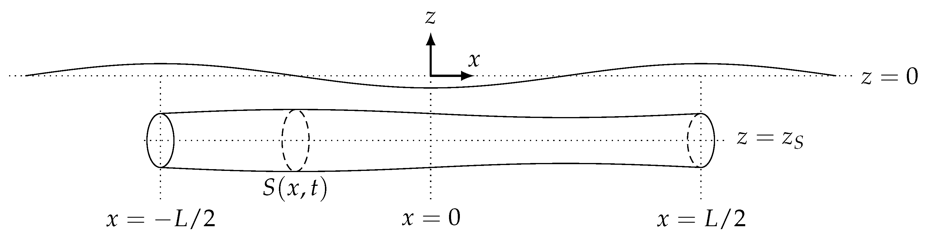
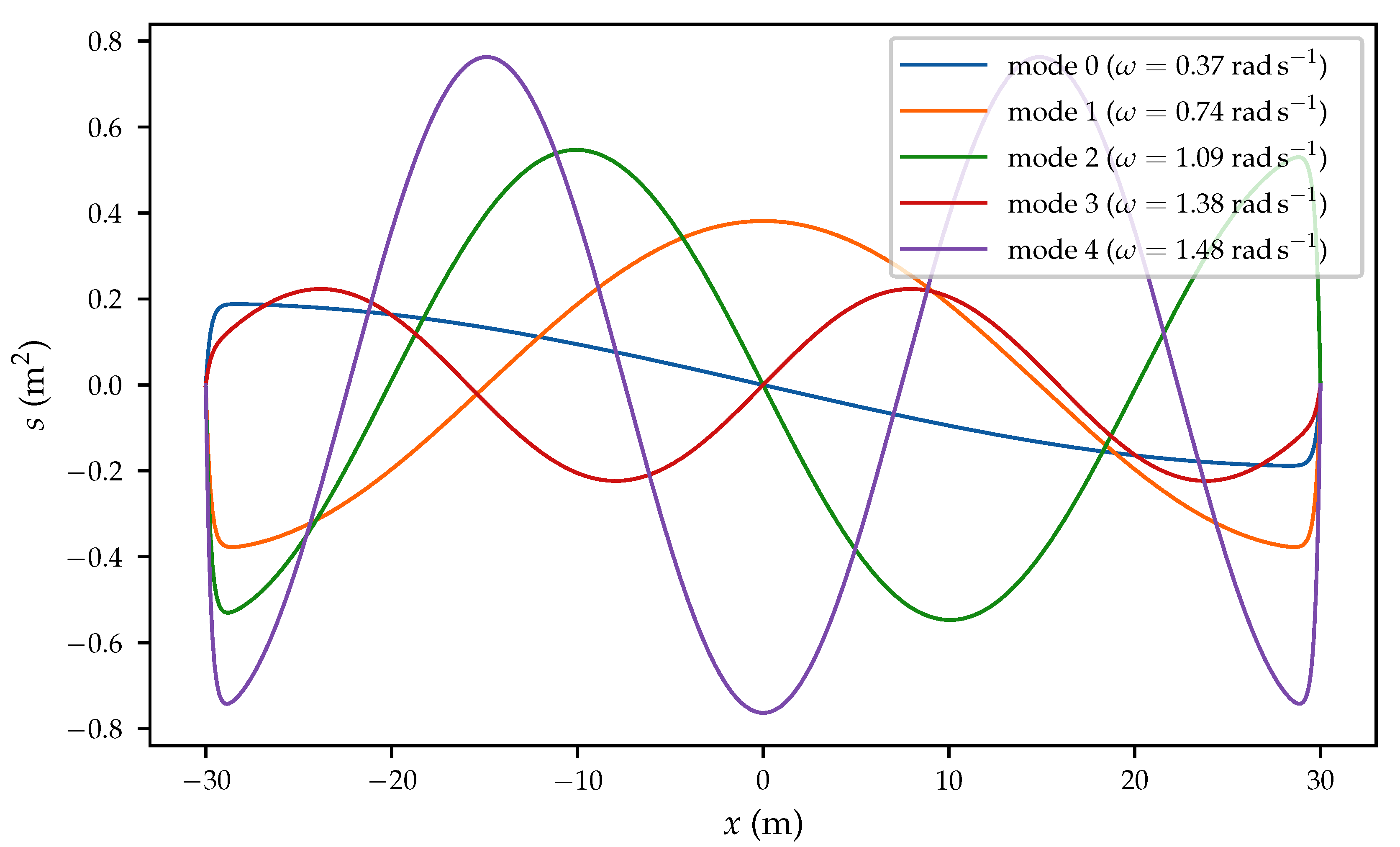
2.3. Modal Analysis of the SBM Offshore’s S3 Device
3. Numerical Results
3.1. Implementation and Setup
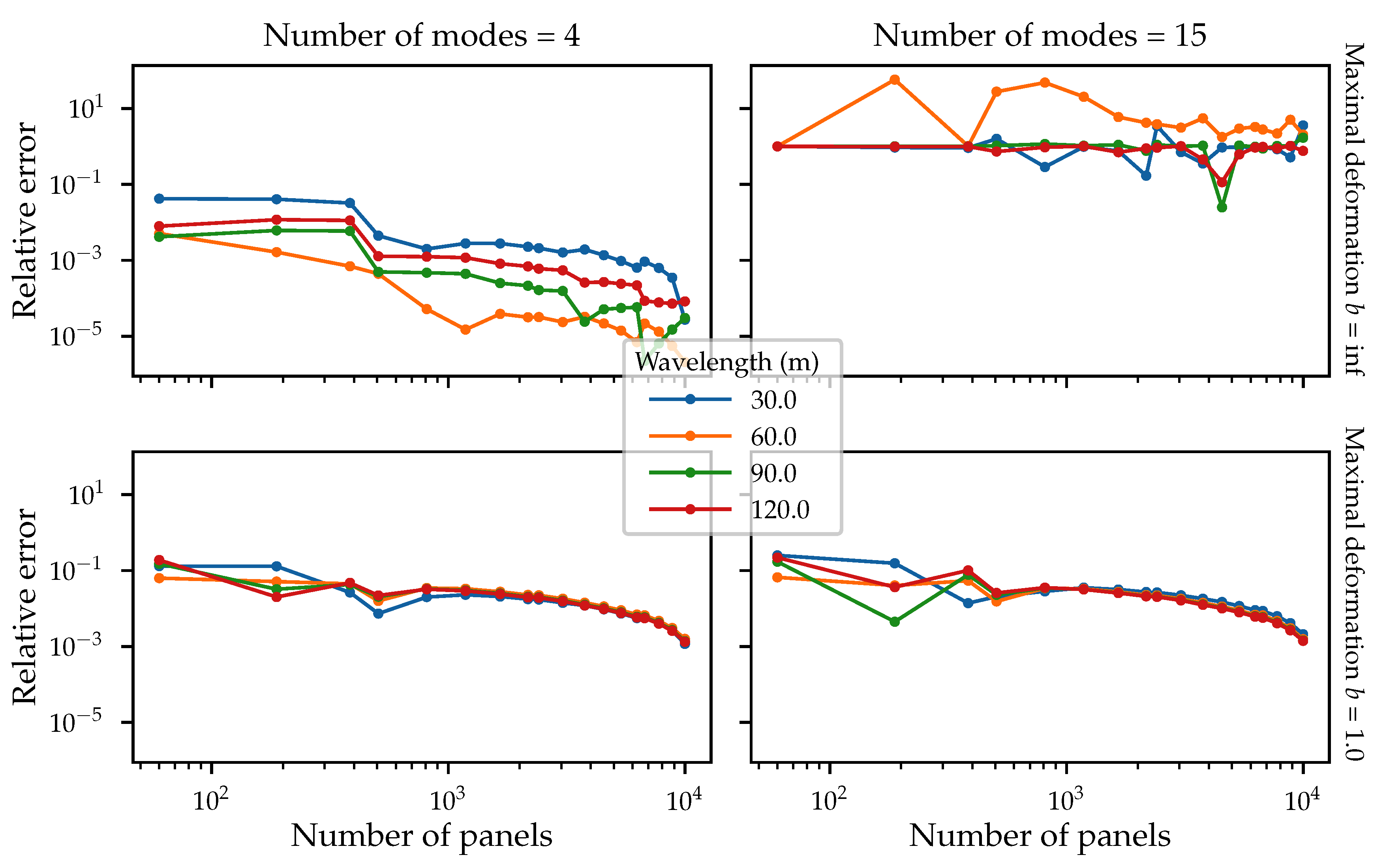
3.2. Mesh Convergence Study
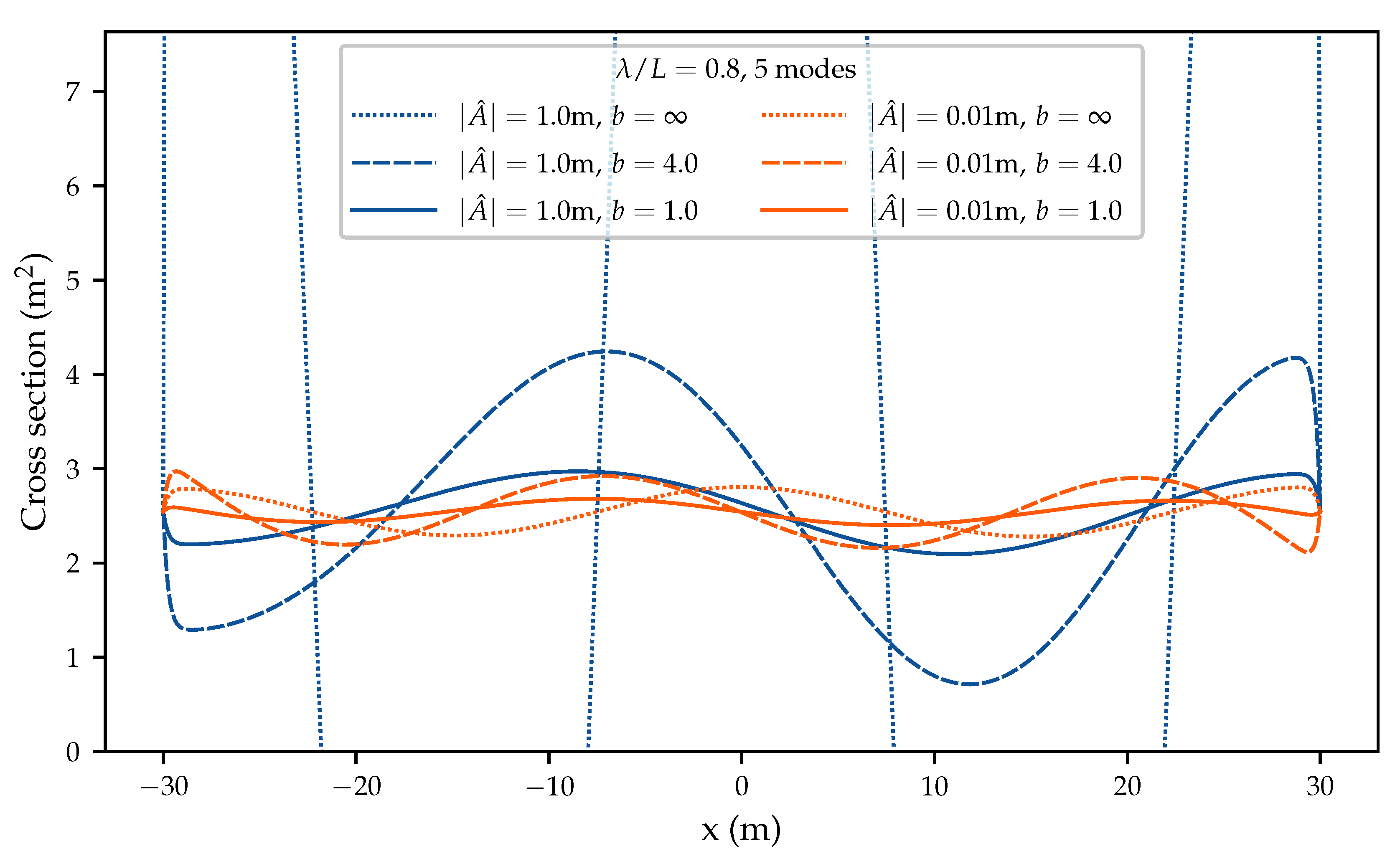
3.3. Examples of Deformation Profiles
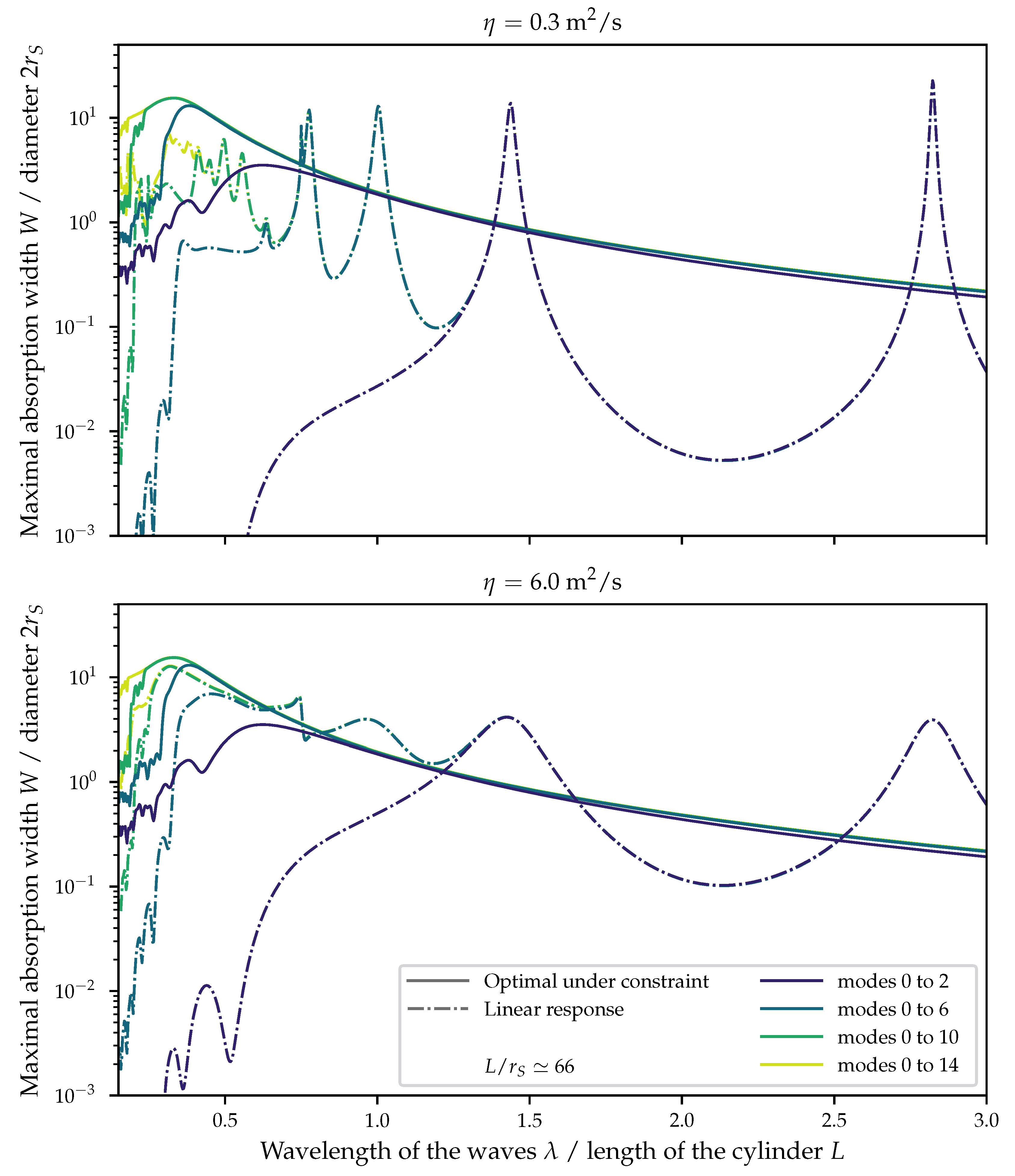
3.4. Maximal Absorption Width with and without Constraint
3.5. Comparison with the Linear Response of the WEC
4. Discussion and Conclusions
Author Contributions
Funding
Acknowledgments
Conflicts of Interest
References
- Desmars, N.; Tchoufag, J.; Younesian, D.; Alam, M.R. Interaction of surface waves with an actuated submerged flexible plate: Optimization for wave energy extraction. J. Fluids Struct. 2018, 81, 673–692. [Google Scholar] [CrossRef]
- Tay, Z.Y.; Wei, Y. Power enhancement of pontoon-type wave energy convertor via hydroelastic response and variable power take-off system. J. Ocean. Eng. Sci. 2020, 5, 1–18. [Google Scholar] [CrossRef]
- Mei, C.C. Nonlinear resonance in Anaconda. J. Fluid Mech. 2014, 750, 507–517. [Google Scholar] [CrossRef]
- Renzi, E. Hydroelectromechanical modelling of a piezoelectric wave energy converter. Proc. R. Soc. A 2016, 472, 20160715. [Google Scholar] [CrossRef] [Green Version]
- Babarit, A.; Singh, J.; Mélis, C.; Wattez, A.; Jean, P. A numerical model for analysing the hydroelastic response of a flexible Electro Active Wave Energy Converter. J. Fluid Struct. 2017, 74, 356–384. [Google Scholar] [CrossRef] [Green Version]
- Folley, M. Numerical Modelling of Wave Energy Converters: State-of-the-Art Techniques for Single Devices and Arrays; Academic Press: Cambridge, MA, USA, 2016. [Google Scholar]
- Babarit, A. Ocean Wave Energy Conversion; Elsevier: Amsterdam, The Netherlands, 2018. [Google Scholar]
- Newman, J. Absorption of wave energy by elongated bodies. Appl. Ocean Res. 1979, 1, 189–196. [Google Scholar] [CrossRef]
- Farley, F. Wave energy conversion by flexible resonant rafts. Appl. Ocean Res. 1982, 4, 57–63. [Google Scholar] [CrossRef]
- Farley, F. Far-field theory of wave power capture by oscillating systems. Philos. Trans. R. Soc. A Math. Phys. Eng. Sci. 2012, 370, 278–287. [Google Scholar] [CrossRef] [PubMed]
- Ancellin, M.; Babarit, A.; Jean, P.; Dias, F. Far Field Maximal Power Absorption of a Bulging Cylindrical Wave Energy Converter: Preliminary Numerical Results. Actes des Journées de l’Hydrodynamique 2018. 2018. Available online: http://website.ec-nantes.fr/actesjh/images/16JH/Articles/JH2018_papier_07D_Ancellin_et_al.pdf (accessed on 15 October 2020).
- Dong, M. Hydro-Elastic Response of a Bulging Cylindrical Wave Energy Converter; Internship Report; University College Dublin: Dublin, Ireland, 2019. [Google Scholar]
- Falnes, J.; Kurniawan, A. Fundamental formulae for wave-energy conversion. R. Soc. Open Sci. 2015, 2, 140305. [Google Scholar] [CrossRef] [PubMed] [Green Version]
- Zheng, S.; Meylan, M.H.; Zhu, G.; Greaves, D.; Iglesias, G. Hydroelastic interaction between water waves and an array of circular floating porous elastic plates. J. Fluid Mech. 2020, 900. [Google Scholar] [CrossRef]
- Ancellin, M.; Dias, F. Capytaine: A Python-based linear potential flow solver. J. Open Source Softw. 2019, 4, 1341. [Google Scholar] [CrossRef]
- Babarit, A.; Delhommeau, G. Theoretical and numerical aspects of the open source BEM solver NEMOH. In Proceedings of the 11th European Wave and Tidal Energy Conference (EWTEC2015), Nantes, France, 6–11 September 2015. [Google Scholar]
- Virtanen, P.; Gommers, R.; Oliphant, T.E.; Haberland, M.; Reddy, T.; Cournapeau, D.; Burovski, E.; Peterson, P.; Weckesser, W.; Bright, J.; et al. SciPy 1.0: Fundamental algorithms for scientific computing in Python. Nat. Methods 2020, 17, 261–272. [Google Scholar] [CrossRef] [PubMed] [Green Version]
- Kraft, D. A software package for sequential quadratic programming. In Forschungsbericht- Deutsche Forschungs- und Versuchsanstalt fur Luft- und Raumfahrt; DFLVR: Oberpfaffenhofen, Germany, 1988; Volume DFLVR-FB 88-28. [Google Scholar]
- Hunter, J.D. Matplotlib: A 2D graphics environment. Comput. Sci. Eng. 2007, 9, 90–95. [Google Scholar] [CrossRef]
- Hoyer, S.; Hamman, J. xarray: N-D labeled arrays and datasets in Python. J. Open Res. Softw. 2017, 5. [Google Scholar] [CrossRef] [Green Version]
- Lam, S.K.; Pitrou, A.; Seibert, S. Numba: A LLVM-Based Python JIT Compiler. In Proceedings of the Second Workshop on the LLVM Compiler Infrastructure in HPC; Association for Computing Machinery: New York, NY, USA, 2015. [Google Scholar] [CrossRef]
- Ancellin, M.; Dias, F. Using the floating body symmetries to speed up the numerical computation of hydrodynamics coefficients with Nemoh. In Proceedings of the 37th International Conference on Ocean, Offshore and Arctic Engineering (OMAE2018), Madrid, Spain, 17–22 June 2018. [Google Scholar] [CrossRef]


| length L | 60 |
|---|---|
| radius | |
| cross section | |
| D | |
| M | 38,000 kg |
| water density | 1025 / |
Publisher’s Note: MDPI stays neutral with regard to jurisdictional claims in published maps and institutional affiliations. |
© 2020 by the authors. Licensee MDPI, Basel, Switzerland. This article is an open access article distributed under the terms and conditions of the Creative Commons Attribution (CC BY) license (http://creativecommons.org/licenses/by/4.0/).
Share and Cite
Ancellin, M.; Dong, M.; Jean, P.; Dias, F. Far-Field Maximal Power Absorption of a Bulging Cylindrical Wave Energy Converter. Energies 2020, 13, 5499. https://doi.org/10.3390/en13205499
Ancellin M, Dong M, Jean P, Dias F. Far-Field Maximal Power Absorption of a Bulging Cylindrical Wave Energy Converter. Energies. 2020; 13(20):5499. https://doi.org/10.3390/en13205499
Chicago/Turabian StyleAncellin, Matthieu, Marlène Dong, Philippe Jean, and Frédéric Dias. 2020. "Far-Field Maximal Power Absorption of a Bulging Cylindrical Wave Energy Converter" Energies 13, no. 20: 5499. https://doi.org/10.3390/en13205499
APA StyleAncellin, M., Dong, M., Jean, P., & Dias, F. (2020). Far-Field Maximal Power Absorption of a Bulging Cylindrical Wave Energy Converter. Energies, 13(20), 5499. https://doi.org/10.3390/en13205499