Development and Validation of CFD 2D Models for the Simulation of Micro H-Darrieus Turbines Subjected to High Boundary Layer Instabilities ^†

Abstract

The simulation of very small vertical axis wind turbines is often a complex task due to the very low Reynolds number effects and the strong unsteadiness related to the rotor operation. Moreover, the high boundary layer instabilities, which affect these turbines, strongly limits their efficiency compared to micro horizontal axis wind turbines. However, as the scientific interest toward micro wind turbine power generation is growing for powering small stand-alone devices, Vertical Axis Wind Turbines (VAWTs)might be very suitable for this kind of application as well. Furthermore, micro wind turbines are widely used for wind tunnel testing, as the wind tunnel dimensions are usually quite limited. In order to obtain a better comprehension of the fluid dynamics of such micro rotors, in the present paper the authors demonstrate how to develop an accurate CFD 2D model of a micro H-Darrieus wind turbine, inherently characterized by highly unstable operating conditions. The rotor was tested in the subsonic wind tunnel, owned by the University of Catania, in order to obtain the experimental validation of the numerical model. The modeling methodology was developed by means of an accurate grid and time step sensitivity study and by comparing different approaches for the turbulence closure. The hybrid LES/RANS Delayed Detached Eddy Simulation, coupled to a transition model, demonstrated superior accuracy compared to the most advanced unsteady RANS models. Therefore, the CFD 2D model developed in this work allowed for a thorough insight into the unstable fluid dynamic operating conditions of micro VAWTs, leading the way for the performance improvement of such rotors.

1. Introduction

The interest for micro wind power generation is growing, since micro wind turbines appear to be very suitable for powering low-power devices such as wireless sensors, actuators, controllers, and small lightning systems. Usually, these devices are powered by means of chemical batteries, which however must be periodically replaced, therefore representing a challenge for a reliable power supply. For this reason, small-size energy harvesters are increasingly used in order to realize reliable self-powered systems. Small-scale wind turbines represent an attractive solution for the electricity generation in such small-size energy harvesters.

Previous studies about miniature wind turbines mainly focused on Horizontal Axis Wind Turbine (HAWT) due to the fact they had acceptable efficiency despite the small scale. Xu et al. [1] developed an experimental test and a numerical predictive model on a miniature HAWT with a diameter of 15 cm. They obtained a maximum efficiency of approximately 27%. Kishore et al. [2,3] designed and characterized a small-scale portable wind turbine of approximately 40 cm that showed very low cut-in velocity and a maximum efficiency of 30% with a rated power of 1.4 W. Zakaria et al. [4] performed an experimental investigation of a centimeter-scale wind turbine, thus showing the strong effect of the very low Reynolds number on the rotor performance as they obtained an efficiency of only 3–4%. An interesting application of miniature HAWT was proposed again by Xu et al. [5]. They developed a physical-based model for the prediction of the optimal load resistance and the experimental characterization of the micro turbine. The efficiency was found to be lower than 10%. Ionescu et al. [6] studied the possibility to optimize small VAWTs through the use of different techniques such as specific low Re airfoils, blade shapes, and passive and active flow control. A special design optimization of a cost-effective micro turbine was implemented by Leung et al. [7]. The multi-bladed rotor, with a radius of approximately 12 cm, reached a maximum power coefficient (C_p) of 12%. Howey et al. [8] designed a miniature shrouded multi-bladed wind turbine by means of the BEM theory. The experimental study result demonstrated a maximum efficiency just over 10%. Park et al. [9] made a feasibility study about the use of micro wind turbines to power wireless sensors on a bridge. They were able to demonstrate how a micro turbine, with a diameter of 14 cm, can generate sufficient energy for this specific application.

Micro wind turbines are often used for wind tunnel experiments as well. As the wind tunnel dimensions are usually limited, only small size rotors can be tested. In this regard, Bastankhah et al. [10] designed and analyzed a miniature wind turbine with a rotor diameter of 15 cm. They demonstrated that an accurate fluid dynamic design for specific low Reynolds number was of utmost importance for reaching high efficiency. In this case they obtained a maximum C_p of approximately 40%. The authors of the present paper presented a numerical and experimental study regarding a three bladed micro HAWT for wind tunnel applications [11]. An efficiency of about 30% was found.

The studies presented above demonstrate the scientific interest toward micro wind rotors and highlight the fact that small rotors need a very accurate fluid dynamic design in order to obtain high efficiency. This is mainly due to two factors. Very low Reynolds numbers drastically reduce the airfoil performances and the small dimensions emphasize the unsteadiness and the instabilities, as will be demonstrated hereinafter. It is no coincidence that VAWTs have not been taken into consideration in the aforementioned studies. Indeed, in these rotors, the unsteady phenomena affect the performance much more than in HAWTs and the scale reduction drastically augments negative effects such as dynamic stall, blade-wake interaction as well as low Reynolds number influence. However, the advantages of VAWTs, such as constructive simplicity, omnidirectionality with respect to the flow, and positioning of the generation unit on the ground, make these turbines deserve further investigation in the aforementioned small-scale applications. For instance, Mutlu et al. [12] evaluated the performance of in-pipe VAWT for turbo solenoid valve system, finding interesting results.

In light of the above, in the present work the authors developed a 2D CFD model of a H-Darrieus VAWT with a diameter of 20 cm. The CFD model was validated by means of wind tunnel experiments carried out in the subsonic wind tunnel at the University of Catania. This micro rotor operated at very low tip speed ratios and very low Re, which caused strong and sudden boundary layer instability (separation and unsteady vortex shedding) leading to early dynamic stall development and large lift losses on the blade. This involved that most of the CFD procedures, proposed in the literature for largest rotors, may not be suitable in this case.

The experimental H-Darrieus rotor had 4 NACA 0012 blades and it was designed and constructed with a 3D printer. Further details about the experimental set up are presented in the next section. In order to develop an accurate and reliable CFD model of such micro rotor, a thorough sensitivity study was carried out. The study analyzed the spatial and temporal discretization sensitivity and the influences of three different turbulence models. The turbulence models evaluated were the widely used RANS fully turbulent SST k-ω model, the transition SST model by Menter, and the hybrid RANS/LES Delayed Detached Eddy Simulation model (DDES) coupled to the transition SST model by Menter for the RANS region. Furthermore, the results were compared to those obtained through the use of a double multiple stream-tube 1D model (DMSTM) using the commercial software Qblade with the suitable aerodynamic polar for an average rotor Reynolds number of approximately 40,000. The global comparison with the experimental data demonstrated that the DDES turbulence model with a very fine spatial and temporal discretization was the one able to provide accurate predictions of the rotor performance in terms of average power coefficient (C_p). The other turbulence models highly underestimated the average C_p despite the very fine spatial and temporal discretization. On the other hand, Qblade DMSTM results demonstrated a surprising proximity to the C_p experimental data, at least in a portion of the curve.

The results obtained through the post-processing of the CFD 2D model allowed the authors to gain an important insight into to the fluid dynamics of micro Darrieus rotors and to clarify the physical reasons for the very poor performance of these turbines when the geometrical scale is reduced. The boundary layer instability, accurately detected through the use of DDES, seemed to be the most important reason for the poor performance of such small rotors. Furthermore, this instability was strongly related to the reduced geometrical scale, which led to very low operating Reynolds numbers. At these very low Re, the boundary layer is mostly laminar and, as is widely known, a laminar boundary layer is more sensitive to adverse pressure gradients that trigger laminar bubbles, separation, and sudden transition.

2. Numerical Model and Experimental Setup

2.1. Literature Background

The CFD 2D numerical model presented in this paper was based on a wide literature background. The literature dealt mainly with larger rotors that in general operated in more stable conditions and higher Reynolds numbers, therefore their 3modelling3 usually led to accurate results. On the other hand, the present study focused on the development of a numerical 3model3 specifically dedicated to micro H-Darrieus rotor in which highly unstable conditions like boundary layer instability, dynamic stall, and blade-wake interaction affected the rotor operation more than in large rotors. However, numerous advices were found in the literature as reported hereinafter. Balduzzi et al. [13,14,15] provided essential guidelines for the development of accurate CFD 2D models of VAWTs, particularly concerning the spatial and temporal independency study. Rezaeiha et al. [16] provided the guidelines for the development of accurate CFD simulations for H-Darrieus rotors, focusing on the domain dimension and the azimuthal increment, which imposed the temporal discretization size. In this case, the authors found a good compromise using a smaller domain than Balduzzi et al. Actually, there is no accordance concerning the computational domain size, which, however, must be sufficiently large to guarantee that the flow around the rotor is not affected by the domain dimensions. Through wind tunnel experiments, Raciti Castelli et al. [17] validated a CFD 3modelling3 strategy, which regarded the near blade spatial discretization depending on the turbulence models. Recently, Rogowski et al. [18] developed a 2D CFD model of a two bladed H-Darrieus rotor. The model was validated using experimental data. Bangaa et al. [19] performed a numerical study on a single bladed VAWT under dynamic stall conditions using CFD. Additionally, the authors of the present paper previously developed a 2D CFD 3model for moderately large H-Darrieus [20], demonstrating the good accuracy of the transition turbulence model by Menter in cases in which the laminar to turbulent boundary layer transition played an essential role.

The above showed that, beyond the domain size, there was no strong agreement about the spatial and temporal discretization as well. All the reviewed papers agreed with the fact that the SST k-ω based turbulence models demonstrated best accuracy among the RANS turbulence models when used with sufficiently refined spatial and temporal discretization. For example, a y⁺ less than one near the blades was universally considered an essential constraint. A time step size, which limited the azimuthal increment to less than 0.5 degree, was equally important. When boundary layer transition phenomena are detected, a transition turbulence model strongly increased the accuracy of the CFD models [20,21]. However, other authors evidenced the superior accuracy of advanced turbulence 4models4 like hybrid RANS-LES formulations, specifically when the rotors are subjected to unstable conditions. Strong dynamic stall, high blade-wake interaction, and vortices related to the flow separation were certainly more accurately predicted through the use of hybrid RANS-LES models like DES and Delayed DES. For example, Lei et al. [22] demonstrated that improved DDES simulation was able to capture real flow characteristics, like those generated by vortices related to dynamic stall phenomena, that were not predicted by the SST k- ω model. Li et al. [23] optimized the blade pitch in a two-blade H-Darrieus turbine using a 2D CFD model based on DDES simulation, therefore evidencing its superior predictive capability with respect to the RANS models. Thè et al. [24], in their thorough review, showed that DDES simulations were the best compromise between high accuracy and computation requirements for the simulation of VAWTs under unstable conditions. Simão Ferreira et al. [25,26] performed a complete numerical-experimental comparison between RANS, DES, and LES turbulence models using accurate Particle Image Velocimetry (PIV) data. They proved that “the DES model is not only able to predict the generation and shedding of vorticity and its convection, it also shows an acceptable sensitivity to grid refinement (both space and time), thus making it suitable for simulations where validation data are limited or non-existent. URANS models proved insufficient because of their inability to correctly model the large eddies, and the influence of this in the development of forces in the downwind passage of the rotor. The LES performed worse than the DES model, probably because of a less accurate 4modelling4 of the wall region.” Again, DDES techniques demonstrated an ability to accurately predict massively separated turbulent flow structures in an Orthopter-type VAWT [27] in which the operating conditions are inherently unstable. Abdellah et al. [28] 4analyzed the effect of the spatial discretization when DDES simulations were implemented for VAWT rotors. Wang et al. [29] also demonstrated the high accuracy of DDES turbulence models for deep dynamic stall simulations at low Reynolds numbers of the NACA 0012 airfoil. The paper fixed grid and time step requirements such that the LES region was able to capture at least 80% of the turbulent kinetic energy of the flow. Furthermore, they evidenced the superior accuracy of the SST transition model for the RANS region among the RANS models at low Reynolds numbers. The above suggested that a DDES, based on a transition formulation for the RANS region, would be the optimal choice for the simulation of airfoil subjected to deep dynamic stall at low Reynolds number. This was certainly the typical operating condition of the H-Darrieus rotor in the present work. This option was studied by Sa et al. [30] on the flow past an Eppler 387 wing. The results indicated that the hybrid DES/Transition model predicted both strong laminar/turbulent transition phenomena, including the laminar separation bubble, and flow separation at high angles of attack. Therefore, the DDES turbulence model with the transition turbulence model by Menter [31,32,33], recently implemented in ANSYS Fluent solver, appeared to be very suitable for the scope of the present work. In order to support this assumption a comparison between the RANS fully turbulent SST k-ω model, the SST transition model and the DDES, coupled to the SST transition model, was carried out in the present paper.

2.2. Computational Domain and Experimental Setup

The experimental rotor was a four bladed H-Darrieus rotor with a ratio between height and diameter equal to one. Two endplates were used for the reduction of the tip losses in such a way to make the experimental results, as much as possible, consistent with the 2D simulations. Even though a 3D simulation would have been very interesting, the computation time would have been unaffordable, therefore a 2D simulation was the only way to gain a thorough insight into the blade aerodynamics. The blades were built in a resin 3D printer, which allowed for very high accuracy of the details and a very fine surface roughness. The endplates were 3D printed in PLA material. A steel threaded bar was used as shaft.

Table 1. Experimental rotor features.

Geometrical and Experimental Details
Diameter (m)	0.2
Height (m)	0.2
Cord (m)	0.03
Number of blades	4
Solidity	0.19
Blade airfoil	NACA 0012
Pitch (deg)	0
Shaft diameter (m)	0.01
Maximum Re	~50,000
Bearings	2 Needle Roller Bearings
Flow speed range (m/s)	11–21
Rotational speed range (r/min)	27–580
Tip speed ratio range	0.025–0.29
Blade attachment point	¼ chord length from LE

reports the geometrical and experimental rotor features while Figure 1 shows an image of the rotor assembled on the experimental setup.

The rotor was widely tested in the subsonic wind tunnel owned by the University of Catania. The wind tunnel was a closed circuit wind tunnel with a test section of 0.5 × 0.5 m, a maximum achievable flow speed of 31 m/s, and a maximum measured turbulent intensity of 0.4%. The test was carried out in open test section configuration. More details about the wind tunnel are reported in [11,34]. The flow speed was measured through the use of a Pitot probe, placed at the center of the test section inlet and at half diameter from it. The rotational speed was measured by means of a digital laser tachometer. The torque was evaluated by using a specifically designed braking system based on the principle of the belt brake. The instantaneous brake force was measured through a load cell and the torque was obtained. The rotor was anchored at the support structure through two needle roller bearings and the torque losses were experimentally evaluated as a function of the rotational speed. To measure the torque, the wind tunnel was set in such a way to obtain the maximum achievable flow speed in open test chamber. The rotor was free to rotate, without braking load, until an equilibrium rotational speed was reached. A constant braking load was then applied, slowing the rotor down until a new equilibrium rotational speed was reached. The net instantaneous breaking force was measured through the load cell, and the average torque for the operating point was calculated. Then, keeping fixed the braking load, the flow speed was reduced by 2 m/s and the new torque was measured each time together with the new equilibrium rotational speed. This process was repeated in steps of 2 m/s until the rotor stopped. The experiment was with three different braking loads, five times for each. In order to obtain the fluid dynamic power, to be compared to the numerical simulation results for the validation, the power losses in the bearings were added at each measured operating point. The flow and rotational speed range is reported in Table 1, while in Figure 2 a sketch of the experimental setup is shown.

The CFD simulations were implemented for five different couples of flow and rotational speed to cover the entire range of measured tip speed ratio. Since there was no agreement about the adequate domain dimensions to have independent results, the first step in the development of the CFD 2D model was the definition of the suitable computational domain. In this case, the best compromise is shown in Figure 3. It was verified that larger domains did not affect the solution further in terms of torque prediction. The use of the symmetry condition for the lateral boundaries reduced the possible influences of the domain dimensions on the flow-field.

The boundary conditions used in the present work are shown in Figure 3. A velocity inlet condition was used for the inlet and a pressure outlet condition for the outlet. For the rotating zone, the domain was divided into three sub-domains in order to implement the unsteady sliding mesh model (SMM) in a rotating ring, which contained the four blades as in [20]. The internal circle and the outer domain remained stationary. The external and internal circumferences of the ring were thus set as sliding interfaces as highlighted in Figure 3.

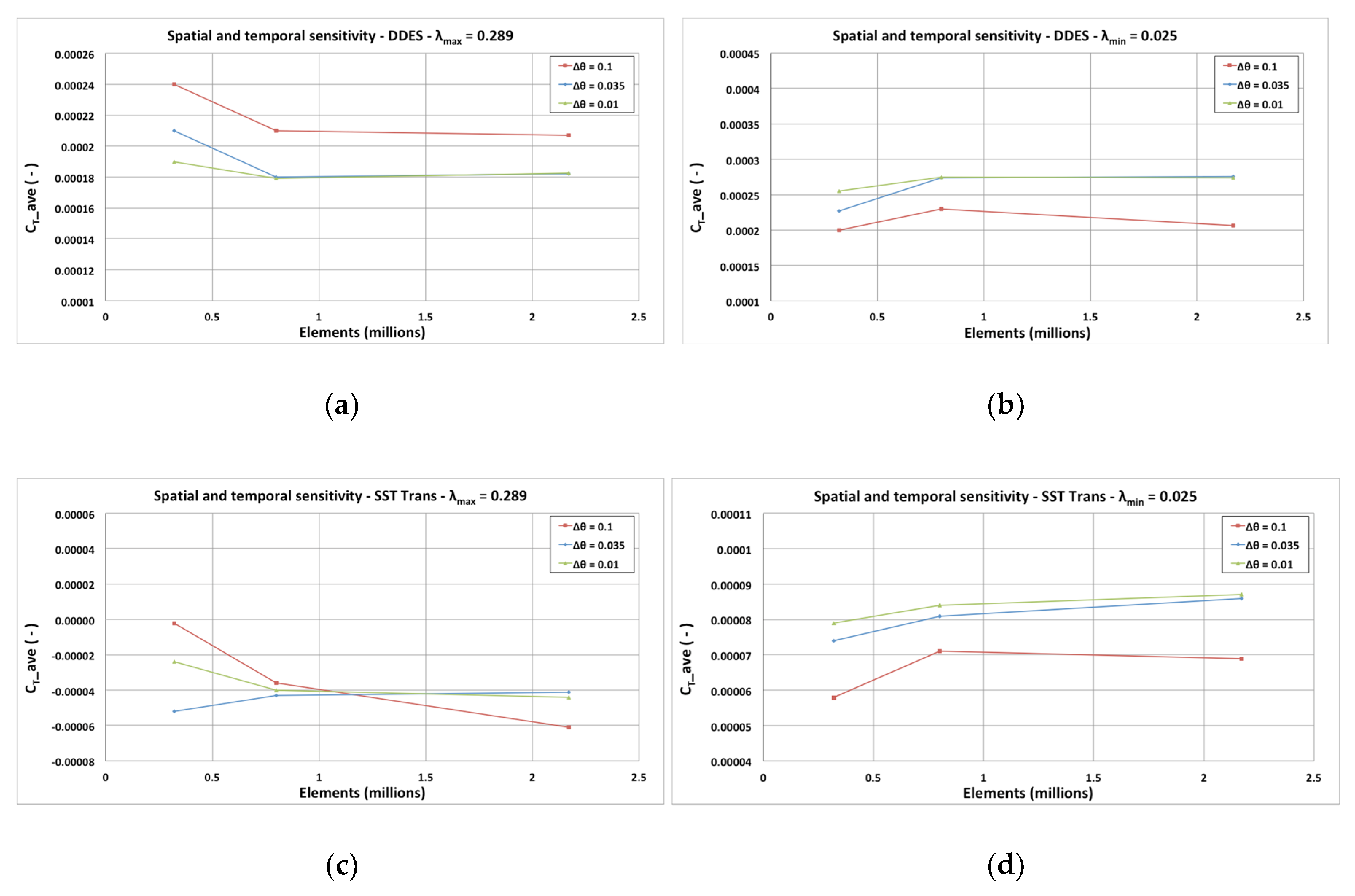
2.3. Spatial and Temporal Sensitivity Study

In order to obtain an adequate level of spatial and temporal discretization, a thorough sensitivity study was made in this work, based on the papers of Balduzzi et al. [13,14,15]. This was done to ensure the best compromise between accuracy and computation time. Specifically, it was suggested in [13,14,15] that, as the tip speed ratio was reduced, the grid refinement must be increased in order to adequately capture the higher vorticity gradients related to the increasing unstable operating conditions [13,14,15]. Furthermore, the temporal discretization must be reduced accordingly to the grid refinement so as the Courant number was below 10, thus providing the optimal error damping properties in the implicit scheme solver used in the present work. Therefore, due to the highly unstable condition related to the very low operating tip speed ratios of the micro rotor analyzed (between 0.025 and 0.29 in Table 1), a specific spatial and temporal sensitivity study was made. The study was carried out for each of the three turbulence models. In this way, the sensitivity of the turbulence models to the grid refinements was evaluated as well. Nine sensitivity tests for each rotor operating condition were made. Three meshing levels and three time steps were tested for each of the three turbulence models. The sensitivity was tested for the maximum (λ = 0.29) and the minimum (λ = 0.025) tip speed ratio in order to find the best compromise for all the intermediate simulations. A global amount of 54 simulations were carried out in this sensitivity study. In this way, an optimal spatial and temporal discretization level was found to be valid for all the simulated operating conditions.

The three grid refinement levels used are reported in

Table 2. Grid independence study meshing characteristics.

Grid Features	Mesh M1	Mesh M2	Mesh M3
Number of elements	320,000	800,000	2,170,000
Nodes on airfoil	1000	2000	4000
Max rotating domain sizing	0.75 mm	0.5 mm	0.25 mm
Max inner circle sizing	0.75 mm	0.5 mm	0.25 mm
Max outer domain sizing	10 mm	10 mm	10 mm
Global growth rate	1.2	1.1	1.05
Inflation layers	20	40	60
First layer height	10−3 mm	10−3 mm	10−3 mm
Skewness max	0.77	0.72	0.79
Y+ max	0.25	0.23	0.22

, where M1 is the coarsest mesh and M3 is the finest one. To refine the mesh, the number of nodes on the airfoil was increased and the cell sizing of the rotating domain was reduced accordingly. The same cell sizing of the rotating ring was imposed to the inner circle to have a very fine discretization leading to an accurate transport of the vortices detached from the upwind blades. This constant fine mesh reduced the numerical diffusion on the upwind blade wakes, thus improving the accuracy of the downwind blade-vortex interactions. Exactly the same refinement was imposed to both the sliding interfaces so as to reduce the interpolation errors at the non-conformal sliding mesh. The boundary layer of the blades was discretized using quadrangular layers of elements. The quadrangular elements allowed for a more accurate resolution of the boundary layer compared to the triangular elements used for the rest of the domain.

The three meshes were developed with a different number of quadrangular layers and growth rates as reported in Table 2. The first layer height was fixed in such a way to guarantee a y⁺ < 1 for all the simulations, as required by the turbulence models [29,31,32,33]. A sizing function, which limited the maximum dimension of the elements, was used in the stationary outer domain as well. The same growth rate as that used for the inflation layers was applied to the whole domain, thus allowing for a gradual mesh coarsening from the rotating interfaces to the boundaries.

In Figure 4, some details of the Mesh M2 are shown. It is worth remarking that Mesh M2 and Mesh M3 did satisfy the Grid Reduced Vorticity (GRV) criterion proposed by Balduzzi et al. [14]. GRV is a quantitative parameter for a qualitative a priori evaluation of the spatial discretization accuracy. GRV is defined as a vorticity normalized with respect to the local grid size, and thus gives an estimate of the velocity variation within a single element. Therefore, it represents the capability of the mesh itself of correctly computing the gradient flow features. The mesh sensitivity analysis and the evaluation of GRV are therefore strictly related: grid independent results are obtained when the discretization error becomes irrelevant, i.e., when GRV is sufficiently small [14]. In the present paper, it was verified that Mesh M2 and Mesh M3 had GRV < 1%, as recommended by [14], while Mesh M1 presented slightly larger values. Furthermore, all three grids satisfied the LES filter constraint imposed by the use of the DDES model, which required to have cell dimension lower than 1/30 the cord length [35].

The temporal discretization must be defined so that all the relevant time scales of the flow were resolved. For this purpose, the time step dimension was chosen in such a way to try a wide set of Courant numbers. The Courant number was defined as:

Co = V ∆t/∆x

(1)

As reported in [14], for VAWTs, V is the peripheral velocity of the airfoil, Δx is the average distance between two cell centroids on the airfoil wall and Δt is the time step. The Courant Number expresses the ratio between the temporal time step (Δt) and the time required by a fluid particle, moving with V velocity, to be convected throughout a cell of dimension Δx.

Since V was the tangential velocity, in order to obtain similar Courant numbers for the different grids and rotational speeds, the time step must be varied together with the tip speed ratio. This obviously involved the angular step being kept constant by reducing the time step with increasing tip speed ratios. In

Table 3. Courant numbers for different grids and time steps at maximum and minimum λ.

Δθ (deg)	Δt (s)	Δx (mm)			λ (-)
		0.03 (M1)	0.015 (M2)	0.0075 (M3)
		Co (-)
0.1	0.00003	6.07	12.15	24.29	0.29
0.035	0.00001	2.02	4.05	8.10
0.01	0.000003	0.61	1.21	2.43
0.1	0.00062	5.84	11.69	23.37	0.025
0.035	0.00021	1.98	3.96	7.92
0.01	0.000062	0.58	1.17	2.34

, the Courant numbers, obtained for different combination of grids and time steps, are shown. Only the finest grids with the largest time step presented slightly high Courant numbers while, in all the other combinations, the Courant numbers were well below 10. This was in order to obtain the best error damping properties, as recommended in [14]. The adaption of the time step was made specifically for all the simulated operating conditions, thus ensuring the same angular step and approximately the same Courant number. In this way, the spatial and temporal discretization was suitable for the specific spatial and temporal scales in each simulation.

The results of the sensitivity study are shown in Figure 5. The charts present the trend of the time-averaged torque coefficient for the various combinations of grids, angular steps and turbulence models. The time-averaged torque coefficient is plotted as a function of the angular steps corresponding to the time steps in Table 3. The number of grid elements is reported on the horizontal axis. Figure 5a,b refers to the DDES model results at maximum (a) and minimum (b) tip speed ratio, respectively. Figure 5c,d refers to the RANS SST transition model while Figure 5e,f shows the RANS SST k-ω model results. The sensitivity analysis demonstrates that the grids M2 and M3 with angular steps Δθ = 0.035° and Δθ = 0.01° lead to results which are in very close proximity to each other, for both λ_max and λ_min. For the DDES turbulence model, the difference is approximately 1%. Therefore, mesh M2 with an angular step equal to Δθ = 0.035° was the best compromise for all the simulated range of tip speed ratio. Specifically, for all the other simulated operating conditions, the time step was adapted to obtain Δθ = 0.035°.

It is already evident that both RANS turbulence models highly underestimate the average torque coefficient with respect to the DDES model. Even negative time-averaged torque coefficients are predicted at λ_max. This would suggest that in highly unstable boundary layer conditions, the RANS turbulence models lead to wrong physical predictions of the flow-field. On the contrary, the DDES model results agreed very well with the experiments as demonstrated in the following sections.

2.4. CFD SOLVER Settings

The CFD solver setup is reported in

Table 4. Main CFD solver settings.

Solver	ANSYS Fluent—Transient—Coupled
Turbulence models	URANS Transition SST URANS SST k-ω Delayed DES with Transition SST
Numerical schemes	Least squares cell based for gradients Second order upwind for all the equations Bounded central differencing for momentum in DDES Second order implicit for time differencing in URANS Bounded second order implicit for time differencing in DDES
Rotation model	Sliding Mesh Model
Iterations per time step	60
Turbulence boundary conditions	Inlet: TI = 0.1%, TVR = 10 Outlet: TI = 5%, TVR = 10
Convergence criterion	Average torque coefficient variation lower than 0.1% between two subsequent revolutions
Simulated operating conditions	Vw = 11.1 m/s	n = 27 r/min	λ = 0.025
	Vw = 15.2 m/s	n = 133 r/min	λ = 0.092
	Vw = 17 m/s	n = 227 r/min	λ = 0.14
	Vw = 19.1 m/s	n = 362 r/min	λ = 0.198
	Vw = 21 m/s	n = 580 r/min	λ = 0.29

. The ANSYS Fluent transient solver was used with a coupled algorithm for pressure-velocity coupling. The three aforementioned turbulence models were tested. Optimized local correlation parameters were used for the SST transition formulation both in URANS and in DDES. This optimization was carried out according to a previous work by the authors [36]. These local correlation parameters triggered and controlled the onset of the laminar to turbulent boundary layer transition within the transport equation for intermittency and momentum thickness Reynolds number. The number of iterations within each time step was set in order to ensure that all the residuals, within each sub-iteration, were well below 10^–4. The turbulence boundary conditions were set according to wind tunnel data and literature suggestions [20]. The convergence criterion was to have a time-averaged torque coefficient variation lower than 0.1% between two consecutive revolutions [14]. This was achieved in about five to ten complete rotor revolutions. Once the convergence was reached, the data were sampled for two consecutive revolutions for the torque time-averaging. The simulated operating conditions are shown in Table 4. The simulations were carried out on a HP Z820 workstation with 24 available cores for parallel calculation and 128 GB of RAM memory. The calculation time per revolution was approximately 58 h with the SST k-ω model, 65 h with the Transition SST model and 71 h with the DDES model.

3. Model Validation and Analysis of the Results

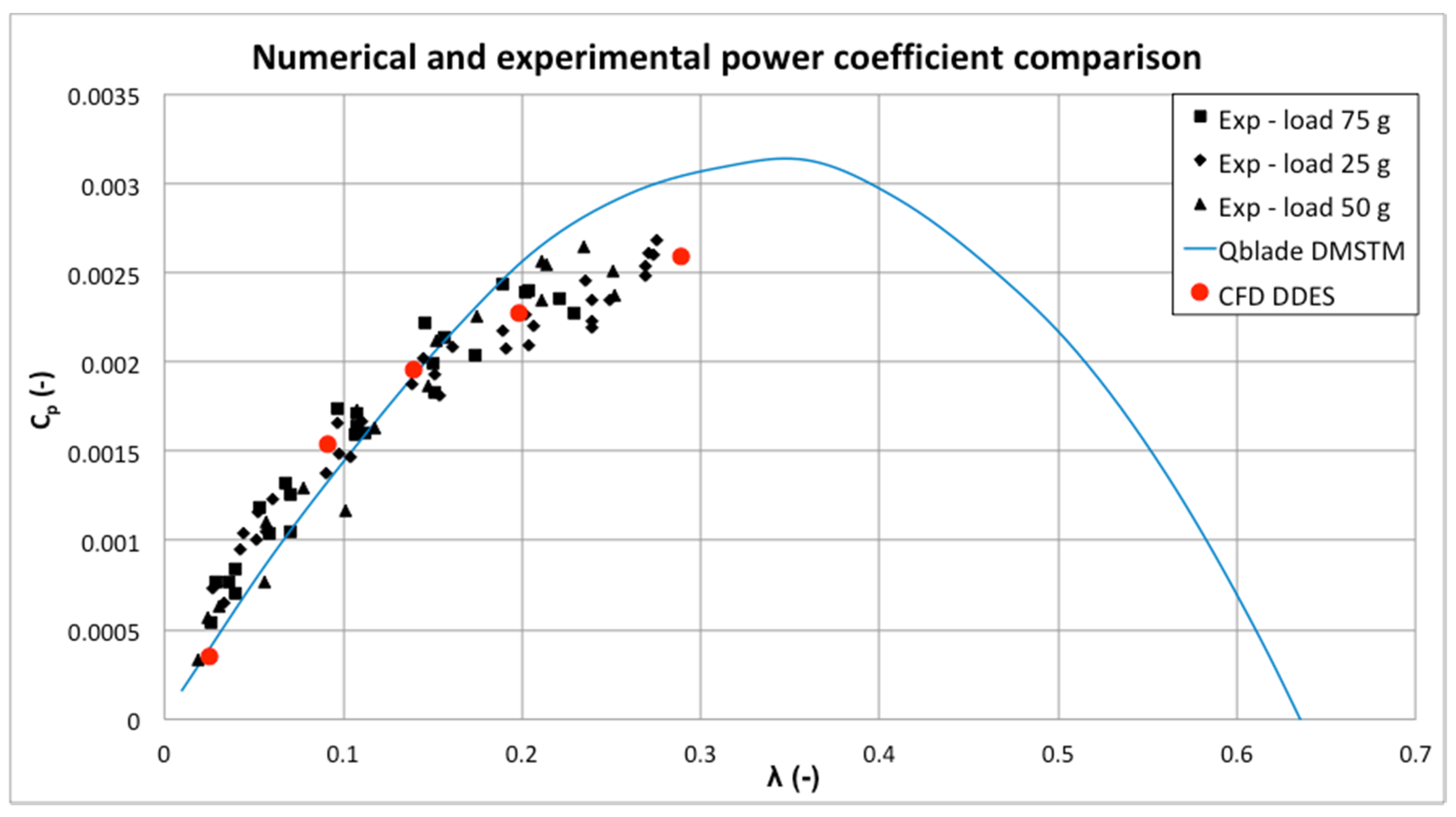
3.1. Experimental Validation of the CFD Model

The experimental tests, carried out in the subsonic wind tunnel owned by the University of Catania, demonstrated that the small VAWT rotor object of this study is much less efficient than a HAWT of comparable size. The maximum measured power of the micro rotor presented here was approximately only 0.55 W at a flow speed of 21 m/s. A micro HAWT with comparable dimensions, tested by the authors in a previous work [11], showed a power of approximately 10 W at the same flow speed.

Concerning the experimental validation of the CFD model, in Figure 6 the comparison between the measured and the calculated power coefficients is shown. The experimental data in Figure 6 refer to the three different braking loads equal to 25 g, 50 g, and 75 g in mass. Due to the low torque generated by the rotor, the torque dissipated by the bearings limited the range of measurement approximately at λ = 0.3. Owing to the unphysical prediction obtained with the RANS turbulence models, only the DDES simulation results are reported in Figure 6. Both the URANS SST transition and SST k-ω model predicted unrealistic negative power coefficients for almost the entire operating range of the rotor. Furthermore, in Figure 6, the Qblade Double Multiple Stream Tube Model (DMSTM) power coefficient prediction is plotted. Qblade is an open source 1D code [37] that required the use of suitable polars for the airfoils. In this case, the experimental data of the NACA 0012 were taken from the literature [38], for an average cord Reynolds number of approximately 40,000. The DMSTM implemented within Qblade uses advanced models and corrections for tip losses, dynamic stall and virtual camber, similar to those used in the BEM theory for HAWTs [39].

The close proximity between experimental measurements and simulation results proved an excellent accuracy of the CFD 2D model based on DDES [40]. Considering the unphysical predictions obtained with the RANS turbulence models despite the very fine spatial and temporal discretization level, this result is very meaningful. In the simulation of strong boundary layer instabilities in VAWTs, the use of an advanced turbulence model like DDES appears to be necessary.

The 1D Qblade results in Figure 6 showed surprising accuracy as well. At least the first part of the C_p curve is well predicted in light of the extreme simplicity and rapidness of the Qblade model. This certainly deserves further investigations on different geometries and operating conditions, in order to verify whether it is a mere chance or a generalizable result.

Nevertheless, CFD still remains the only way to get a thorough insight into the rotor aerodynamics, which is of utmost importance for the comprehension of the causes of the poor efficiency of such micro VAWTs. For this purpose, the present work demonstrated that only an advanced turbulence modeling like the hybrid RANS-LES formulation, implemented in DDES, was able to provide accurate and physically reliable results. Moreover, the availability of an accurate CFD model will allow the authors to identify an optimization strategy for these rotors in order to increase their efficiency. The use of more suitable airfoils, specific pitch angles, and vortex generators are just some of the simplest and cheapest techniques, whose effectiveness will be evaluated thanks to the CFD model developed in this work.

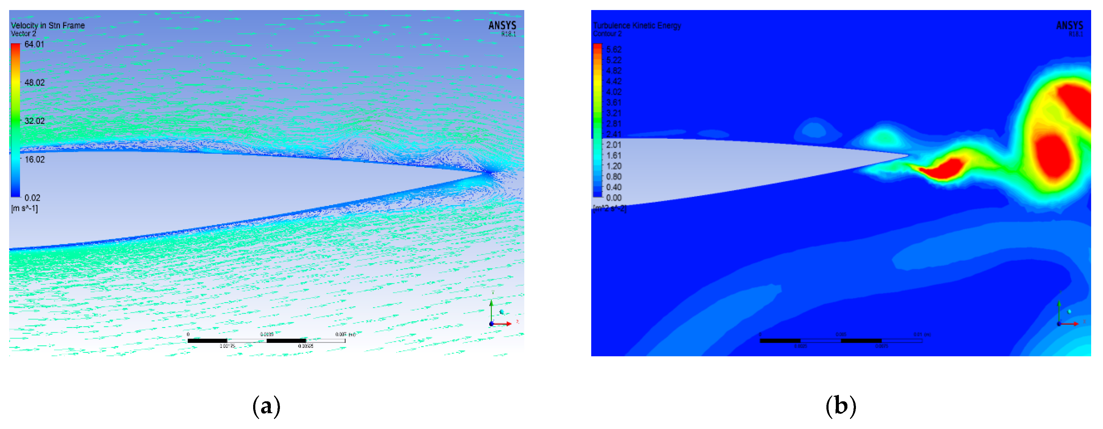
3.2. Post-Processing and Analysis of the Results

A thorough post-processing analysis of the flow-field in terms of velocity, turbulence production, and vorticity was carried out for two specific azimuthal rotor positions evidenced in Figure 7. In blue, the instantaneous position named as “position 0°” in which the blades are located at θ = 0°, 90°, 180°, and 270°. In red, the instantaneous position named as “position 45°” in which the blades are located at θ = 45°, 135°, 225°, and 315°. In this way the analysis is quite representative of the rotor behavior within a revolution. Only the λ_max condition results are presented as the other operating conditions lead to very similar considerations. The images showed hereinafter explain both the reasons for the poor accuracy of the RANS turbulence models and the low efficiency of these rotors.

In Figure 8, the contours of velocity magnitude for the three turbulence models demonstrate the strong differences in the flow-field prediction. The DDES results (Figure 8a) demonstrate the capability to accurately capture structures which are smaller and more defined than those obtained from the RANS simulations. Indeed, the RANS models seem to diffuse the swirling structures more than the DDES model. This result was expectable since the LES modeling inside the DDES was inherently more accurate. Furthermore, the flow separation dynamic of the blades at azimuthal positions θ = 90° and 270° appears to be different, also between the transition and the SST k-ω models. In this condition, indeed, the transition model predicted larger scale vortices compared to the SST k-ω model. The above suggests that the RANS models overestimate the dimensions of the flow structures and their diffusion within the grid. Therefore, the negative effects of unsteady phenomena like dynamic stall and blade-vortex interaction, in the down-wind sector, would be probably overestimated as well. For example, the blade at θ = 0° shows a recirculation area near the trailing edge in Figure 8b,c, which is larger than that in Figure 8a. This seems to denote that the RANS models in this case of micro rotor, tend to predict an earlier flow separation, which in turn results in higher turbulence production and finally lower torque. Considering the fact that both the RANS models predicted negative torque at λ_max, while the DDES showed excellent accuracy, it can be supposed that the RANS models led to unphysical flow-field predictions. A possible explanation may be related to the fact that the small dimensions of the rotor generate flow structures that the RANS averaging is not able to capture despite the very high spatial and temporal discretization. Thus, the more advanced physical solution provided by the DDES model appears to be more suitable in the case of such micro rotors.

The contours of turbulent intensity for the three turbulence models in Figure 9 further confirm this assumption. The RANS models predict a massive and smoothed turbulence production. The DDES model instead predicts much less turbulence production in smaller and more defined structures. The massive turbulence production of the RANS models results in high rotor energy dissipation, which is not realistic. Moreover, the large turbulence structures in Figure 9b,c produce much more influences on the downwind blades than those in the DDES model. This further confirms that the physics beyond the RANS models does not seem to be suitable for the simulation of the highly unstable conditions related to such small rotors.

The vorticity field presented in Figure 10 shows very different results between the three turbulence models. Again, the DDES (Figure 10a) demonstrate the capability to predict more defined and less smoothed structures but with much higher vorticity within the cores of the shed vortices, compared to the RANS model results. In light of the widely known capability of the LES to accurately predict the eddies behavior, and thanks to the excellent numerical-experimental agreement evidenced in Figure 6, the DDES model appears to be more physically realistic. In cases like that in the present work, in which the operating conditions are massively dominated by unstable shedding of vortices, the RANS modeling clearly leads to wrong physical predictions. This issue is reduced on larger rotors in which more stable flow-field conditions lead to less shedding of vortices, and therefore to a better physical agreement of the RANS models.

Similar considerations can be made for the position 45°. In Figure 11, Figure 12 and Figure 13 the contours of velocity magnitude, the contours of turbulence intensity, and the contours of vorticity are shown, respectively. In this case, all the blades are subjected to angles of attack such that the flow is fully separated. The differences between the DDES and the RANS results are even more evident. The velocity field appears smoother in the RANS compared to the DDES. In Figure 12, the massive unrealistic turbulence production, predicted by the RANS models, is even higher than in Figure 9, with respect to the DDES results. The contours of Figure 13 confirm the complexity of the vorticity field predicted by the DDES simulation, compared to the smoothed and less complex structures obtained thorough the RANS simulations.

The accuracy demonstrated by the DDES results allows for an insight into the poor efficiency that characterizes such micro rotors. Figure 8, Figure 9 and Figure 10a show that the blade at the azimuthal position θ = 0° is just affected by an incipient boundary layer instability even though the local AoA is approximately 0°. A shedding of vortices is already clearly evident in the airfoil wake.

In this regard, the details reported in Figure 14a,b clarify this assumption. The velocity vectors show boundary layer instabilities, which generate a consistent turbulent kinetic energy production. This is probably due to the low Reynolds number and the related strong sensitivity of the laminar boundary layer to the adverse pressure gradients. This earlier instability leads also to earlier flow separation, which can emphasize the negative effects of the dynamic stall as the blade moves towards higher azimuthal positions. Since the instability limits the attached flow condition phase, the blade azimuthal angle phases in which high lift to drag ratios are achievable are very limited as well. This means that the rotor operates under stall conditions for almost the entire blade rotation. As the blades are subjected to separation for most of the rotation, the dynamic stall, which inherently affects VAWTs, develops more than in large rotors, thus causing higher cyclic losses. The chart in Figure 15 reports the trend of the local blade AoA as a function of the azimuthal blade position, calculated by means of Qblade code at different tip speed ratios. Despite the fact that Qblade results are not as accurate, they provide a fast estimation of the local blade AoA during a complete rotor revolution. The rapid increase of the local AoA is related to the low peripheral speed, which in turn is due to the low torque produced, caused by the aforementioned instability.

Figure 16 further confirms the above considerations. The velocity vectors (a), the contours of turbulent kinetic energy (b) and the pressure coefficient (c) for a blade at azimuthal position θ = 15° are shown. In this specific condition, at λ_max = 0.29, the local blade AoA is approximately 8°. Despite the low AoA, the velocity vectors demonstrate an extensive area of instability, in the form of a kind of laminar bubble, near the trailing edge of the suction side of the blade. This instability produces high turbulent kinetic energy (Figure 16b), which increases the energy dissipation. The pressure coefficient in Figure 16c, calculated with respect to the flow velocity at inlet, shows the effects of these bubbles on the pressure distribution over the suction side of the blade. This in turn impacts negatively on the lift generated by the blade. As the blade moves toward higher azimuthal positions, the instability rapidly moves toward the leading edge, thus influencing the entire suction side of the blade with large flow separation and massive production of swirling structures. The subsequent onset of the dynamic stall further worsens the aerodynamic performance of the blade.

Thus, summarizing, the most important macroscopic evidence for the poor performance of micro H-Darrieus rotors is the fact that the turbine cannot accelerate sufficiently even at high flow speed. The cause of this is essentially due to the precocity with which boundary layer instability and separation occur in terms of AoAs. The very low Reynolds numbers, due to the small dimensions, seem to be the main responsible factor for this early instability, which manifests itself through massive production of vortices and turbulence. Furthermore, the early separation affects the development of the dynamic stall, since the range of AoAs in which it can be triggered is certainly wider. All these effects strongly limit the lift generation as they represent a source of cyclic losses. Moreover, the small dimensions of the radius do not allow for the generation of sufficient torque so that the rotor is not able accelerate at tangential speeds such to overcome the instabilities.

4. Summary and Conclusions

Although one may think micro wind turbines are of little scientific and industrial interest, the literature analysis in the present paper demonstrates that micro rotors represent an attractive solution for small size energy harvesters in many industrial applications. However, at such small scales, the advantages of the vertical axis solution are reduced by the poor rotor efficiency due to the onset of highly unstable boundary layer conditions as the rotor size decreases. The possibility to thoroughly analyze the fluid dynamic causes of the poor efficiency certainly represents a key step for the improvement of these micro rotors. Furthermore, in general, the simulation of the unstable conditions of VAWTs, which arise at low tip speed ratio, is still a very complex problem.

For these reasons, in this work, the authors present the implementation of a 2D CFD model for the simulation of a micro VAWT designed, constructed and tested in the subsonic wind tunnel of the University of Catania. For this purpose, three different turbulence models were evaluated: the SST Transition and SST k-ω RANS models and the hybrid RANS/LES Delayed DES. The thorough temporal and spatial discretization sensitivity study demonstrated that a very fine spatial and temporal discretization was necessary in order to capture the high vorticity gradients related to the unstable conditions, and thus to obtain independent results. While the RANS SST Transition model and SST k-ω model both led to unphysical torque predictions, the Delayed Detached Eddie Simulation, coupled to a transition formulation for the RANS region, was able to accurately reproduce the measured power coefficient.

The thorough post-processing comparison between the RANS and the DDES model results allowed for the identification of the reasons of the poor accuracy of the RANS models. In the highly unstable conditions related to micro rotors, both the RANS models predicted a massive turbulence production which was smoothed in large structures according to the inherent characteristics of the Reynolds averaging. The DDES model instead predicted a higher vorticity but in smaller and more defined swirling structures, leading to much lower turbulence production, and hence lower energy dissipation. In light of the excellent agreement between the DDES and the experimental results, it could be concluded that, in general, for a reliable simulation of the unstable condition of VAWTs the advanced DDES model appear to be the most suitable. However, a fine spatial and temporal discretization is needed to resolve the high vorticity gradients near the blades.

However, the most important result of this work was that the DDES, with transitional treatment for the RANS region, allowed for a thorough insight into the causes of the poor performance of micro H-Darrieus rotors. The small radius of these rotors together with the low cord Reynolds numbers of the blades involved the onset of early separation and boundary layer instabilities. These phenomena constantly affected the micro rotor operating conditions also because of a wider development of the dynamic stall for large part of the azimuthal blade position. All this involved a significant limitation of the torque generated since the rotor operated under high cyclic losses. The negative impact of the reduction of the geometrical scale was evidently much more significant in Darrieus VAWT than in HAWT.

The results of the present work provide some guidelines for the improvement of the efficiency of micro VAWTs as well. First of all, the use of specific low Reynolds number airfoils could reduce the onset of the instabilities, therefore allowing for higher torque generation and, therefore, higher rotational speeds. Different blade pitch angles may be more efficient in these small rotors than in the larger rotors. Simple variable blade pitch systems could be easily and cheaply applied to these rotors thanks to 3D printers. All this will be investigated in detail in future works.

References

1. Xu, F.J.; Yuan, F.-G.; Liu, L.; Hu, J.Z.; Qiu, Y.P. Performance Prediction and Demonstration of a Miniature Horizontal Axis Wind Turbine. J. Energy Eng. 2013, 139, 143–152. [Google Scholar] [CrossRef]
2. Kishore, R.A.; Coudron, T.; Priya, S. Small-scale wind energy portable wind turbine (SWEPT). J. Wind Eng. Ind. Aerodyn. 2013, 116, 21–31. [Google Scholar] [CrossRef] [Green Version]
3. Kishore, R.A.; Priya, S. Design and eperimental verification of a high efficiencysmall wind energy portable turbine (SWEPT). J. Wind Eng. Ind. Aerodyn. 2013, 118, 12–19. [Google Scholar] [CrossRef]
4. Zakaria, M.Y.; Pereira, D.A.; Hajj, M.R. Experimental investigation and performance modeling of centimeter-scale micro-wind turbine energy harvesters. J. Wind Eng. Ind. Aerodyn. 2015, 147, 58–65. [Google Scholar] [CrossRef]
5. Xu, F.J.; Yuan, F.G.; Hu, J.Z.; Qiu, Y.P. Miniature horizontal axis wind turbine system for multipurpose application. Energy 2014, 75, 216–224. [Google Scholar] [CrossRef]
6. Ionescu, R.D.; Szava, I.; Vlase, S.; Ivanoiu, M.; Munteanu, R. Innovative solutions for portable wind turbines, used on ships. Procedia Technol. 2015, 19, 722–729. [Google Scholar] [CrossRef]
7. Leung, D.Y.C.; Deng, Y.; Leung, M.K.H. Design Optimization of a Cost-Effective Micro Wind Turbine. In Proceedings of the World Congress on Engineering (WCE 2010), London, UK, 30 June–2 July 2010; Volume 2, pp. 988–993. [Google Scholar] [CrossRef] [Green Version]
8. Howey, D.A.; Bansal, A.; Holmes, A.S. Design and performance of a cm-scale shrouded wind turbine for energy harvesting. Smart Mater. Struct. 2011, 20, 85021. [Google Scholar] [CrossRef] [Green Version]
9. Park, J.W.; Jung, H.-J.; Jo, H.; Spencer, B.F., Jr. Feasibility Study of Micro-Wind Turbines for Powering Wireless Sensors on a Cable-Stayed Bridge. Energies 2012, 5, 3450–3464. [Google Scholar] [CrossRef] [Green Version]
10. Bastankhah, M.; Porté-Agel, F. A New Miniature Wind Turbine for Wind Tunnel Experiments. Part I: Design and Performance. Energies 2017, 10, 908. [Google Scholar] [CrossRef] [Green Version]
11. Lanzafame, R.; Mauro, S.; Messina, M. Numerical and experimental analysis of micro HAWTs designed for wind tunnel applications. Int. J. Energy Environ. Eng. 2016, 7, 199. [Google Scholar] [CrossRef] [Green Version]
12. Mutlu, Y.; Çakan, M. Evaluation of in-pipe turbine performance for turbo solenoid valve system. Eng. Appl. Comput. Fluid Mech. 2018, 12, 625–634. [Google Scholar] [CrossRef]
13. Balduzzi, F.; Bianchini, A.; Maleci, R.; Ferrera, G.; Ferrari, L. Critical issues in the CFD simulation of Darrieus wind turbines. Renew. Energy 2016, 85, 419–435. [Google Scholar] [CrossRef]
14. Balduzzi, F.; Bianchini, A.; Ferrara, G.; Ferrari, L. Dimensionless numbers for the assessment of the mesh and timestep requirements in CFD simulations of Darrieus wind turbines. Energy 2016, 97, 246–261. [Google Scholar] [CrossRef]
15. Bianchini, A.; Balduzzi, F.; Bachant, P.; Ferrara, G.; Ferrari, L. Effectiveness of two-dimensional CFD simulations for Darrius VAWTs: A combined numerical and experimental assessment. Energy Convers. Manag. 2017, 136, 318–328. [Google Scholar] [CrossRef]
16. Rezaeiha, A.; Kalkman, I.; Blocken, B. CFD simulation of a vertical axis wind turbine operating at a moderate tip speed ratio: Guidelines for minimum domain size and azimuthal increment. Renew. Energy 2017, 107, 373–385. [Google Scholar] [CrossRef] [Green Version]
17. Castelli, M.R.; Ardizzon, G.; Battisti, L.; Benini, E.; Pavesi, G. Modeling strategy for a Darrieus vertical axis micro-wind turbine. In Proceedings of the ASME 2010 International Mechanical Engineering Congress & Exposition IMECE2010-39548, Vancouver, BC, Canada, 12–18 November 2010; pp. 409–418. [Google Scholar] [CrossRef]
18. Rogowski, K.; Hansen, M.O.L.; Lichota, P. 2-D CFD Computations of the Two-Bladed Darrius-Type Wind Turbine. J. Appl. Fluid Mech. 2018, 11, 835–845. [Google Scholar] [CrossRef]
19. Bangga, G.; Huotomo, G.; Wiranegara, R.; Sasongko, H. Numerical study on a single bladed vertical axis wind turbine under dynamic stall. J. Mech. Sci. Technol. 2017, 31, 261–267. [Google Scholar] [CrossRef]
20. Lanzafame, R.; Mauro, S.; Messina, M. 2D CFD modeling of H-Darrieus wind turbines using a transition turbulence model. Energy Procedia 2014, 45, 131–140. [Google Scholar] [CrossRef] [Green Version]
21. Mannion, B.; Leen, S.B.; Nash, S. A two and three-dimensional CFD investigation into performance prediction and wake characterization of a vertical axis turbine. J. Renew. Sustain. Energy 2018, 10, 34503. [Google Scholar] [CrossRef]
22. Lei, H.; Zhou, D.; Bao, Y.; Li, Y.; Han, Z. Three-dimensional Improved Delayed Detached Eddy Simulation of a two-bladed vertical axis wind turbine. Energy Convers. Manag. 2017, 133, 235–248. [Google Scholar] [CrossRef]
23. Li, C.; Xiao, Y.; Xu, Y.; Peng, Y.; Hu, G.; Zhu, S. Optimization of blade pitch in H-rotor vertical axis wind turbines through computational fluid dynamics simulations. Appl. Energy 2018, 212, 1107–1125. [Google Scholar] [CrossRef]
24. Thé, J.; Yu, H. A critical review on the simulations of wind turbine aerodynamics focusing on hybrid RANS-LES methods. Energy 2017, 138, 257–289. [Google Scholar] [CrossRef]
25. Ferreira, C.J.S.; Bijl, H.; van Bussel, G.; van Kuik, G. Simulating Dynamic Stall in a 2D VAWT: Modeling strategy, verification and validation with Particle Image Velocimetry data. J. Phys. Conf. Ser. 2007, 75, 12023. [Google Scholar] [CrossRef] [Green Version]
26. Ferreira, C.J.S.; van Zuijlen, A.; Bijl, H.; van Bussel, G.; van Kuik, G. Simulating dynamic stall in a two-dimensional vertical-axis wind turbine: Verification and validation with particle image velocimetry data. Wind Energ. 2010, 13, 1–17. [Google Scholar] [CrossRef]
27. Elkhoury, M.; Kiwata, T.; Nagao, K.; Kono, T.; Elhajj, F. Wind tunnel experiments and Delayed Detached Eddy Simulation of a three-bladed micro vertical axis wind turbine. Renew. Energy 2018, 129, 63–74. [Google Scholar] [CrossRef]
28. Abdellah, B.; Belkheir, N.; Khelladi, S. Effect of Computational Grid on Prediction of a Vertical axis Wind turbine Rotor Using Delayed Detached-Eddy Simulations. In Proceedings of the 2018 International Conference on Wind Energy and Applications in Algeria (ICWEAA), Algiers, Algeria, 6–7 November 2018; pp. 1–5. [Google Scholar] [CrossRef]
29. Wang, S.; Ingham, D.B.; Ma, L.; Pourkashanian, M.; Tao, Z. Turbulence modeling of deep dynamic stall at relatively low Reynolds number. J. Fluids Struct. 2012, 33, 191–209. [Google Scholar] [CrossRef]
30. Sa, J.H.; Park, S.H.; Kim, C.J.; Park, J.K. Low-Reynolds number flow computation for eppler 387 wing using hybrid DES/transition model. J. Mech. Sci. Technol. 2015, 29, 1837–1847. [Google Scholar] [CrossRef]
31. Menter, F.R.; Langtry, R.; Volker, S. Transition modeling for general purpose CFD codes. Flow Turb. Combust. 2006, 77, 277–303. [Google Scholar] [CrossRef]
32. Langtry, R.B.; Menter, F.R.; Likki, S.R.; Suzen, Y.B.; Huang, P.G.; Volker, S. A Correlation-Based Transition Model Using Local Variables—Part I: Model Formulation. In Proceedings of the ASME Turbo Expo 2004: Power for Land, Sea, and Air, Vienna, Austria, 14–17 June 2004. [Google Scholar]
33. Langtry, R.B.; Menter, F.R.; Likki, S.R.; Suzen, Y.B.; Huang, P.G.; Volker, S. A correlation-based transition model using local variables—Part II: Test cases and industrial applications. ASME J. Turbomach. 2006, 128, 423–434. [Google Scholar] [CrossRef]
34. Brusca, S.; Lanzafame, R.; Messina, M. Low speed wind tunnel: Design and build. In Wind Tunnels: Aerodynamics, Models and Experiments; Pereira, J.D., Ed.; Nova Science Publishers, Inc.: Hauppauge, NY, USA, 2011; ISBN 978-1-61209-204-1. [Google Scholar]
35. Spalart, P.R. Young-Person’s Guide to Detached-Eddy Simulation Grids; NASA/CR-2001-211032; NASA Langley Research Center: Hampton, VA, USA, 2001.
36. Mauro, S.; Lanzafame, R.; Messina, M.; Pirrello, D. Transition turbulence model calibration for wind turbine airfoil characterization through the use of a Micro-Genetic Algorithm. Int. J. Energy Environ. Eng. 2017, 8, 359–374. [Google Scholar] [CrossRef] [Green Version]
37. Marten, D.; Wendler, J.; Pechlivanoglou, G.; Nayeri, C.N.; Paschereit, C.O. Qblade: An open source tool for design and simulation of horizontal and vertical axis wind turbines. Int. J. Emerg. Technol. Adv. Eng. 2013, 3, 264–269. [Google Scholar]
38. Shedahl, R.E.; Klimas, P.C. Aerodynamic Characteristics of Seven Symmetrical Airfoil Sections through 180-Degree Angle of Attack for Use in Aerodynamic Analysis of Vertical Axis Wind Turbines; Technical Report No. SAND80-2114; Sandia National Laboratories: Albuquerque, NM, USA, 1981.
39. Lanzafame, R.; Mauro, S.; Messina, M. HAWT design and performance evaluation: Improving the BEM therory mathematical models. Energy Procedia 2015, 82, 172–179. [Google Scholar] [CrossRef] [Green Version]
40. Mauro, S.; Brusca, S.; Lanzafame, R.; Messina, M. Micro H-Darrieus wind turbines: CFD modeling and experimental validation. AIP Conf. Proc. 2019, 2191. [Google Scholar] [CrossRef]
Figure 1. Experimental rotor.
Energies 13 05564 g001
Figure 2. Experimental setup and detail of the mechanical brake system.
Energies 13 05564 g002
Figure 3. Computational domain dimensions and boundary conditions.
Energies 13 05564 g003
Figure 4. Details of the rotor region (a), airfoil region (b) leading edge (c) and trailing edge (d) for mesh M2.
Energies 13 05564 g004
Figure 5. Average torque coefficient sensitivity analysis at λmax for DDES (a), SST Trans (c), SST kω (e) and at λmin for DDES (b), SST Trans (d), SST kω (f).
Energies 13 05564 g005aEnergies 13 05564 g005b
Figure 6. Comparison between numerical and experimental power coefficient.
Energies 13 05564 g006
Figure 7. Azimuthal rotor position reference for the post-processing analysis.
Energies 13 05564 g007
Figure 8. Contours of velocity magnitude for DDES (a), RANS Transition (b) and RANS SST k-ω (c) at 0° azimuthal position at λmax = 0.29.
Energies 13 05564 g008
Figure 9. Contours of turbulent intensity for DDES (a), RANS Transition (b) and RANS SST k-ω (c) at 0° azimuthal position at λmax = 0.29.
Energies 13 05564 g009aEnergies 13 05564 g009b
Figure 10. Contours of vorticity for DDES (a), RANS Transition (b) and RANS SST k-ω (c) at 0° azimuthal position at λmax = 0.29.
Energies 13 05564 g010
Figure 11. Contours of velocity magnitude for DDES (a), RANS Transition (b) and RANS SST k-ω (c) at 45° azimuthal position at λmax = 0.29.
Energies 13 05564 g011
Figure 12. Contours of turbulent intensity for DDES (a), RANS Transition (b) and RANS SST k-ω (c) at 45° azimuthal position at λmax = 0.29.
Energies 13 05564 g012aEnergies 13 05564 g012b
Figure 13. Contours of vorticity for DDES (a), RANS Transition (b) and RANS SST k-ω (c) at 45° azimuthal position at λmax = 0.29.
Energies 13 05564 g013aEnergies 13 05564 g013b
Figure 14. Velocity vectors (a) and contours of turbulence kinetic energy (b) for a blade at θ = 0° and λmax = 0.29.
Energies 13 05564 g014
Figure 15. Qblade calculated local AoA as a function of the azimuthal blade position for different tip speed ratios.
Energies 13 05564 g015
Figure 16. Velocity vectors (a), contours of turbulence kinetic energy (b) and pressure coefficient (c) for a blade at azimuthal position θ = 15° and λmax = 0.29.
Energies 13 05564 g016