Discrete-Time DC-Link Voltage and Current Control of a Grid-Connected Inverter with LCL-Filter and Very Small DC-Link Capacitance

Abstract

The paper presents a controller design for grid-connected inverters (GCI) with very small dc-link capacitance that are coupled to the grid via an LCL filter. The usual controller designs would fail and result in instability. The proposed controller has a cascaded structure with a current controller as inner control loop and an outer dc-link voltage controller. The controller design is performed in discrete time and it is based on a detailed stability analysis of the dc-link voltage controller to determine the controller parameters which guarantee stability for all operating points. The inner loop is a state-feedback current controller that is designed based on the discrete linear-quadratic regulator (DLQR) theory. An additional integral error feedback assures steady-state accuracy of the current control loop. The simulation and experimental results validate performance and stability of proposed controller design.

1. Introduction

Grid-connected inverters (GCI) or grid-connected converters (GCC) are part of e.g., (i) Back-to-Back (B2B) converters as used in wind energy conversion systems (WECS), (ii) active front-ends as used in certain drive applications, (iii) grid-connected battery storage systems, or (iv) PV systems. GCI or GCC are used to convert the electrical energy between dc-link and three-phase ac grid and share a common dc-link with e.g., the machine-side converter in WECS or the DC/DC converter in battery or PV systems. Hence, a bidirectional power flow is possible. Because of this, the dc-link capacitor needs to be dimensioned with care and, usually, is oversized.

The shared dc-link capacitance of a GCI or GCC is usually approximately five to ten times greater than the capacitance of a unidirectional converter with similar power rating. In

Table 1. Exemplary literature overview of used sizes of dc-link capacitors.

Ref.	${\mathit{C}}_{\mathbf{dc}}$	${\mathit{u}}_{\mathbf{dc},\mathbf{ref}}$	${\mathit{f}}_{\mathbf{sw}}$	${\mathit{S}}_{\mathbf{nom}}$ ($\mathbf{V}\mathbf{A}$)/${\mathit{P}}_{\mathbf{nom}}$ ($\mathbf{W}$)	Filter
[1]	25 $\mathsf{\mu }$$\mathrm{F}$	700 $\mathrm{V}$	32 $\mathrm{k}$$\mathrm{Hz}$	15 $\mathrm{k}$$\mathrm{V}$$\mathrm{A}$	L
[1]	101 $\mathsf{\mu }$$\mathrm{F}$	700 $\mathrm{V}$	4 $\mathrm{k}$$\mathrm{Hz}$	15 $\mathrm{k}$$\mathrm{V}$$\mathrm{A}$	L
[2]	40 $\mathsf{\mu }$$\mathrm{F}$	450 $\mathrm{V}$	6 $\mathrm{k}$$\mathrm{Hz}$	9 $\mathrm{k}$$\mathrm{W}$	L
[3]	80 $\mathsf{\mu }$$\mathrm{F}$	750 $\mathrm{V}$	5 $\mathrm{k}$$\mathrm{Hz}$	15 $\mathrm{k}$$\mathrm{V}$$\mathrm{A}$	L
[8]	470 $\mathsf{\mu }$$\mathrm{F}$	≥565 $\mathrm{V}$	5 $\mathrm{k}$$\mathrm{Hz}$	$5.5$$\mathrm{k}$$\mathrm{V}$$\mathrm{A}$	L
[9]	470 $\mathsf{\mu }$$\mathrm{F}$	400–450 $\mathrm{V}$	20 $\mathrm{k}$$\mathrm{Hz}$	$1.8$$\mathrm{k}$$\mathrm{W}$	LCL
[10]	800 $\mathsf{\mu }$$\mathrm{F}$	235–450 $\mathrm{V}$	20 $\mathrm{k}$$\mathrm{Hz}$	1 $\mathrm{k}$$\mathrm{W}$	LCL
[11]	$2·500$ $\mathsf{\mu }\mathrm{F}$	600 $\mathrm{V}$	10 $\mathrm{k}$$\mathrm{Hz}$	$2.4$$\mathrm{k}$$\mathrm{W}$	LCL
[12]	1000 $\mathsf{\mu }$$\mathrm{F}$	600 $\mathrm{V}$	-	2 $\mathrm{k}$$\mathrm{W}$ (jumps)	LCL
[13]	1500 $\mathsf{\mu }$$\mathrm{F}$	700 $\mathrm{V}$	-	12 $\mathrm{k}$$\mathrm{W}$	L
[14]	1500 $\mathsf{\mu }$$\mathrm{F}$	680 $\mathrm{V}$	10 $\mathrm{k}$$\mathrm{Hz}$	15 $\mathrm{k}$$\mathrm{V}$$\mathrm{A}$	LCL
[15]	1500 $\mathsf{\mu }$$\mathrm{F}$	800 $\mathrm{V}$	-	6 $\mathrm{k}$$\mathrm{W}$	LCL
[16]	2800 $\mathsf{\mu }$$\mathrm{F}$	400 $\mathrm{V}$	20 $\mathrm{k}$$\mathrm{Hz}$	5 $\mathrm{k}$$\mathrm{V}$$\mathrm{A}$	L
[17]	6000 $\mathsf{\mu }$$\mathrm{F}$	700 $\mathrm{V}$	-	25 $\mathrm{k}$$\mathrm{W}$	LCL
[18]	23,000 $\mathsf{\mu }$$\mathrm{F}$	1200 $\mathrm{V}$	20 $\mathrm{k}$$\mathrm{Hz}$	$1.5$$\mathrm{M}$$\mathrm{W}$	L
[19]	25,000 $\mathsf{\mu }$$\mathrm{F}$	1750 $\mathrm{V}$	4 $\mathrm{k}$$\mathrm{Hz}$	$2.5$$\mathrm{M}$$\mathrm{W}$	LCL
[20]	25,000 $\mathsf{\mu }$$\mathrm{F}$	500 $\mathrm{V}$	15 $\mathrm{k}$$\mathrm{Hz}$	$7.5$$\mathrm{k}$$\mathrm{W}$	LCL
[21]	300,000 $\mathsf{\mu }$$\mathrm{F}$	700 $\mathrm{V}$	-	$1.5$$\mathrm{M}$$\mathrm{W}$	L
[22]	1100 $\mathsf{\mu }$$\mathrm{F}$	150 $\mathrm{V}$	20 $\mathrm{k}$$\mathrm{Hz}$	≤1 $\mathrm{k}$$\mathrm{W}$	L
[23]	1100 $\mathsf{\mu }$$\mathrm{F}$	800 $\mathrm{V}$	10 $\mathrm{k}$$\mathrm{Hz}$	20 $\mathrm{k}$$\mathrm{V}$$\mathrm{A}$	L
[24]	2000 $\mathsf{\mu }$$\mathrm{F}$	680 $\mathrm{V}$	10 $\mathrm{k}$$\mathrm{Hz}$	15 $\mathrm{k}$$\mathrm{V}$$\mathrm{A}$	LCL
[25]	3300 $\mathsf{\mu }$$\mathrm{F}$	750 $\mathrm{V}$	5 $\mathrm{k}$$\mathrm{Hz}$	$17.5$$\mathrm{k}$$\mathrm{V}$$\mathrm{A}$	LCL

, an overview of the sizes of the dc-link capacitor and other crucial system parameters is given. Only three references [1,2,3] use similarly small capacitors as used in this paper ($C_{\mathrm{dc}}=60 \mathsf{\mu }\mathrm{F}$), but do not employ an LCL filter.

Using small capacitances (instead of large ones) comes with several benefits: because the dc-link capacitor is used to store energy and to stabilize the dc-link voltage, usually large electrolyte capacitors are used. Those capacitors are less reliable due to their electrolyte usually leading to a shorter lifetime. Additionally, small dc-link capacitors are less bulky and reduce system cost, volume and weight [2,4]. One the other hand, small dc-link capacitances increase the requirements on the underlying control system significantly in order to ensure a stable and proper operation of the GCI.

Besides this, a filter is needed in order to suppress high order harmonics, caused by the steep switching slopes in converters and to meet the total harmonic distortion (THD) limits of respective grid codes. An LCL filter is a third-order filter and it provides a better damping characteristic than commonly used L filters. The better damping allows for smaller component values and smaller sizes as well as less power losses and better system dynamics [5]. When considering high power applications, the switching frequency of the converter is lower and thus the amount of current harmonics increase. Suppressing these harmonics by an L filter requires an excessive inductor value and size. In contrast, the main drawback of LCL filters is its resonance frequency, which may result in system instability. The resonance can be handled by an active method (e.g., by a proportional feedback of the filter capacitor current) or a passive method (e.g., by an additional damping resistor) [6,7]. As an additional resistor increases losses and costs, in this paper, an active damping method is used and incorporated in controller design.

As already mentioned, in e.g., WECS or electrical drive applications, the VSIs can be labeled regarding their location as machine-connected inverter (MCI) or GCI. This paper focuses on the control of the GCI with LCL filter. Several previous efforts and approaches have focused on continuous-time control strategies. The whole system is controlled by a cascaded controller structure. The inner control-loop objectives are power or current flow between the grid-connected inverter and the grid. The objective of the outer control loop is dc-link voltage control. Due to that, preceding studies either deal with the inner current control loop only or the complete (cascaded) control system.

In [26], a power controller, which consists of two proportional-integral (PI) controllers, is presented. Due to a variable transformation into the rotating $(d,q)$-reference frame, the transformed quantities become constant values and there is no stationary error. The disadvantages of this scheme are the necessary implementation of a phase-locked loop (PLL) and the arising cross-coupling terms, which can be eliminated by an additional compensation method. By using the stationary $(\alpha ,\beta )$-reference frame, a PLL is not needed, as shown in [27], but a frequency-looked loop (FLL) is usually still required [28,29]. In this case, the references are sinusoidal and, therefore, a quasi proportional-resonant (QPR) controller must be implemented. There are no cross-coupling terms, but existing harmonic distortion of the grid currents need to be suppressed by harmonic compensators separately. Each harmonic order requires an extra compensation [28,29]. In [9], also a continuous-time dc-link voltage droop controller for a single-phase GCI with LCL filter is proposed. Besides the controller, a special sensing technique is presented, which calculates the mean value of the dc-link voltage. Therefore the controller can be equipped with a higher bandwidth leading to a better controller performance. However, since the sensing technique needs at least one period to estimate the mean value, the controller will react rather slowly and with delay. Furthermore, Ref. [9] presents two enhanced power controllers based on the droop controller. Namely, an adaptive controller approach, taking the instantaneous dc-link current and grid amplitude into account and an optimized controller approach which minimizes the system power losses. In [23], a robust design procedure of a voltage-oriented PI control with virtual resistor based active damping (AR-VD), which is a special method of active damping, for a GCI with LCL filter is presented. The capacitor currents are fed back and used for the virtual resistor based active damping in order to stabilize the system. A simple PI controller is implemented to regulate the dc-link voltage. Ref. [22] focuses on an adaptive dc-link voltage PI controller for a GCI with L filter. The self-tuning controller adapts both its proportional and integral gain, depending on the operating point of the system. The controller is designed to fulfill a fast dynamic response after a reference step of the dc-link voltage as well as of the input current without any overshoot. At an experimental test-bench, the controller is implemented and compared to a classical dc-link PI controller and it shows superior performance. In [30], a Lyapunov-based controller design is proposed that achieves a high robustness against parameter uncertainties and grid distortions. In [11,19], the whole control system is considered and a cascaded PI controller design in the rotating $(d,q)$-reference frame is presented. Drawbacks of these controller designs are their passive damping methods which lead to reduced efficiency. Moreover, the approximation of the LCL filter by a simple L filter is an over-simplification. Other studies focus on a mixture of nonlinear and linear controller designs, as in [17], where a sliding mode controller is combined with an outer PI controller or use pure nonlinear controller designs. Applied methods are backstepping [20,31,32] or input/output-linearization [12].

In conclusion, all of the papers above do their analysis in the continuous-time domain and do not explicitly discuss and analyze stability in view of (i) a small ratio between switching and resonance frequency and (ii) a small dc-link capacitance. Moreover, all of these studies are based on the assumption that the system behavior can be described and the controller tuning can be done in the continuous-time domain sufficiently well. This assumption is satisfied if high sampling and switching frequencies $f_{\mathrm{s}}$, $f_{\mathrm{sw}}$ (in $\mathrm{Hz}$) are used compared to the dominant system frequency (or bandwidth) $f_{\max }$ (in $\mathrm{Hz}$). In the literature, different requirements on the ratio between these frequencies for a quasi-continuous controller design can be found [33]; e.g., a ratio of $f_{\mathrm{s}}\ge 8f_{\max }$ is considered sufficient. If such ratios are not achievable, the controller must be designed based on a system description in discrete time.

In [34], a discrete-time current controller is developed. The system is discretized by the step invariant method. The designed control system represents an internal model control (IMC), which is optimized by a linear matrix inequality (LMI). Two interesting control approaches are presented in [14,24]. Both were applied to a B2B converter, which interconnects two electrical networks via LCL filters. In [24], a unified converter and filter model is presented and, based on which, a linear-quadratic regulatur (LQR) is designed. More enhanced is the discrete LQR (DLQR) controller design in [14]. The controller features fast active and reactive power control as well as a stiff dc-link voltage regulation. The controller shows robustness against variations of the filter parameters, dc-link capacitance, grid inductance, and grid voltage amplitude. The design is based on a power flow model of the two VSCs and their common dc-link capacitor. Common and differential power and current are introduced. A system discretization was performed with the introduced quantities and a linearization around an operating point. An additional integral feedback allows for stationary accuracy and is considered in the DLQR controller design. In [35], solely a DLQR current controller for a single-phase GCI with LCL filter is proposed. The current controller is designed by using linear matrix inequality conditions. The dc-link voltage is assumed to be constant and, hence, a dc-link voltage controller is not even considered. Finally, in [25], a similar control approach is presented for a GCI with LCL filter while using a DLQR current controller and a dc-link voltage PI controller. However, the design of the PI controller is not presented and neither a stability analysis nor recommendations on controller tuning are provided.

Other control strategies are based on predictive or fuzzy control. In [36], a generalized predictive current controller with passive damping is proposed. The studies [37,38] focus on model predictive current control of the GCI. In [39], two finite-control-set (FCS)-MPC algorithms for current control are proposed and evaluated for a GCI with LCL filter. They were called PCi${}_1$i${}_2$u${}_{\mathrm{c}}$ and PCi${}_1$i${}_2$u${}_{\mathrm{c}}$-2steps. Both of the algorithms are based on a cost function, which considers the converter current, the grid current and the capacitor voltage of the LCL filter. The PCi${}_1$i${}_2$u${}_{\mathrm{c}}$-2steps is a more enhanced version of the first algorithm. It has a longer prediction horizon and it is motivated by the third-order system dynamics of the LCL filter. Additionally, here, a dc-link voltage controller is not designed or implemented. A hybrid approach combining a classical controller and an MPC is presented in [40]. A cascaded controller structure, called resonant-predictive control is used to control a GCI with LCL filter. Here, a PR controller is cascaded with a FCS-MPC to merge the benefits of both strategies. The outer PR controller regulates the grid current and its output is the reference signal of the filter capacitor voltage for the inner FCS-MPC loop. The cost function considers the filter capacitor voltage and the converter current. Because a PR controller is used no steady-state tracking error is present and the FCS-MPC achieves a good control performance due to the absence of a modulator as well as an inherent active damping of the filter resonance. Because MPC algorithms usually require feedback of many quantities (=many sensors), [41] investigates an MPC approach with a reduced amount of sensors. A FCS-MPC algorithm is proposed based on estimated values generated from a virtual flux observer and a state observer. Additionally, a delay compensation is implemented. The virtual flux observer is used to estimate the grid voltage and the reference value of the grid current, which are then used by the state observer to estimate the remaining system states. Finally, the FCS-MPC is applied in order to calculate the new switching states. A different digital controller is presented in [15], which uses a Takagi-Sugeno-Kang (TS) fuzzy controller to control active and reactive power.

All of the contributions above rely on (i) a rather large dc-link capacitance (see Table 1) and/or (ii) a rather large ratio between switching frequency and filter resonance frequency (in e.g., [35], this ratio is 20,040 Hz/1744 Hz = 11.5, which shows that a discrete-time controller design is actually not needed). This paper focuses on the control of a GCI with a very small dc-link capacitor and an LCL filter where the resonance frequency is very close to the switching frequency. Both require a well designed and tuned control system. Because of the low switching frequency close to the critical resonance frequency of the LCL filter, a discrete-time controller design is presented. In contrast to most available controller designs, no filter approximation or simplifying assumptions are imposed. Moreover, in contrast to previous works in this area (see above), this paper thoroughly discusses the stability of the discrete-time closed-loop system and validates the findings of the stability analysis by several measurement results. Overall, this paper comes with the following two main contributions:

• The design of a cascaded discrete-time controller structure for a GCI under harsh system conditions such as (a) low sampling frequency close to the resonance frequency of the LCL filter and (b) very small dc-link capacitance.
• A thorough stability analysis and experimental validation of the discrete-time closed-loop system to ensure local stability for several worst-case scenarios and operating points.

This paper is structured, as follows: Section 2 discusses the model of the considered system, which consists of the LCL filter and the GCI, including the small dc-link capacitor. The inner current control loop is designed and analyzed in Section 3. A detailed tuning procedure based on a stability analysis for the outer dc-link voltage control loop can be found in Section 4. The paper concludes with the validation of the proposed theoretical results in Section 5 by comparing the simulation and measurement results and the conclusion in Section 6.

2. System Model

Figure 1 shows the considered system (based on [42]) which needs to be modeled. The LCL filter consists of the inductances $L_{\mathrm{f}}$ and $L_{\mathrm{g}}$ (in $\mathrm{H}$), the filter capacitances $C_{\mathrm{c}}$ (in $\mathrm{F}$) and their parasitic series resistances $R_{\mathrm{f}}$, $R_{\mathrm{g}}$ and $R_{\mathrm{c}}$ (in $\mathrm{\Omega }$), respectively. The GCI is assumed to have six ideal switches, where the lower switch of each phase has the complementary switching state of the respective upper switch, i.e., ${\overline{s}}_{\mathrm{f}}^x=1-s_{\mathrm{f}}^x$ for phase $x\in \{a,b,c\}$ where $s_{\mathrm{f}}^x\in \{0,1\}$ is the switching signal of the upper switch. This means, for example, that the upper switch of phase a is closed if $s_{\mathrm{f}}^a=1$ and open if $s_{\mathrm{f}}^a=0$. Vice versa, in view of ${\overline{s}}_{\mathrm{f}}^a=1-s_{\mathrm{f}}^a$, the lower switch of phase a is closed (i.e., ${\overline{s}}_{\mathrm{f}}^a=1$) if $s_{\mathrm{f}}^a=0$ and open (i.e., ${\overline{s}}_{\mathrm{f}}^a=0$) if $s_{\mathrm{f}}^a=1$. The capacitor $C_{\mathrm{dc}}$ (in $\mathrm{F}$) describes the total dc-link capacitance that was concentrated in one component. The system states are the filter inductance currents ${\mathit{i}}_{\mathrm{f}}^{abc}:={(i_{\mathrm{f}}^a,i_{\mathrm{f}}^b,i_{\mathrm{f}}^c)}^{\top }$ (in $\mathrm{A}$), the grid inductance currents ${\mathit{i}}_{\mathrm{g}}^{abc}:={(i_{\mathrm{g}}^a,i_{\mathrm{g}}^b,i_{\mathrm{g}}^c)}^{\top }$ (in $\mathrm{A}$), the filter capacitance voltages ${\mathit{u}}_{\mathrm{c}}^{abc}:={(u_{\mathrm{c}}^a,u_{\mathrm{c}}^b,u_{\mathrm{c}}^c)}^{\top }$ (in $\mathrm{V}$), and the dc-link voltage $u_{\mathrm{dc}}$ (in $\mathrm{V}$). The inverter output voltages ${\mathit{u}}_{\mathrm{f}}^{abc}:={(u_{\mathrm{f}}^a,u_{\mathrm{f}}^b,u_{\mathrm{f}}^c)}^{\top }$ (in $\mathrm{V}$) will be the actuating variables to the filter, which are generated by space-vector modulation (SVM). The LCL filter is coupled to the grid having grid voltages ${\mathit{u}}_{\mathrm{g}}^{abc}:={(u_{\mathrm{g}}^a,u_{\mathrm{g}}^b,u_{\mathrm{g}}^c)}^{\top }$ (in $\mathrm{V}$).

The bode plot of the LCL filter dynamics in the rotating $(d,q)$-reference frame is shown in Figure 2 for both system inputs, $u_{\mathrm{f}}^d$ and $u_{\mathrm{f}}^q$, respectively. Two different system behaviors are obtained, which depend on the chosen system output (either $i_{\mathrm{f}}^d$, $i_{\mathrm{f}}^q$ or $i_{\mathrm{g}}^d$, $i_{\mathrm{g}}^q$). The transfer functions are given as follows [43]

$$\begin{array}{c}\hfill G_{\mathrm{f}}\left(s\right)=\frac{i_{\mathrm{f}}^d\left(s\right)}{u_{\mathrm{f}}^d\left(s\right)}=\frac{i_{\mathrm{f}}^q\left(s\right)}{u_{\mathrm{f}}^q\left(s\right)}=\frac{s^2{L}_{\mathrm{g}}{C}_{\mathrm{c}}+1}{s^3{L}_{\mathrm{f}}{L}_{\mathrm{g}}{C}_{\mathrm{c}}+s(L_{\mathrm{f}}+L_{\mathrm{g}})}\mathrm{and}{G}_{\mathrm{g}}\left(s\right)=\frac{i_{\mathrm{g}}^d\left(s\right)}{u_{\mathrm{f}}^d\left(s\right)}=\frac{i_{\mathrm{g}}^q\left(s\right)}{u_{\mathrm{f}}^q\left(s\right)}=\frac{1}{s^3{L}_{\mathrm{f}}{L}_{\mathrm{g}}{C}_{\mathrm{c}}+s(L_{\mathrm{f}}+L_{\mathrm{g}})},\end{array}$$

(1)

if parasitic resistances $R_{\mathrm{f}}$, $R_{\mathrm{g}}$ and $R_{\mathrm{c}}$ in filter, grid, and capacitor are neglected. The transfer function $G_{\mathrm{f}}$ has a zero at approximately 750 $\mathrm{Hz}$. Both transfer functions, $G_{\mathrm{f}}$ and $G_{\mathrm{g}}$, have their resonance frequency at $f_{\mathrm{res}}\approx 1255\mathrm{Hz}$, which corresponds to the imaginary part of their complex-conjugated poles. Within a narrow bandwidth of about 40 $\mathrm{Hz}$ around this resonance frequency, the current is amplified (>0 dB) significantly and not damped. This can lead to instability if not a proper controller/tuning is used. For frequencies above the resonance frequency, the transfer function $G_{\mathrm{g}}$ is damped with $60\frac{\mathrm{dB}}{\mathrm{dec}}$, as it is a third-order low-pass filter. Because the numerator of the transfer function $G_{\mathrm{f}}$ does additionally depend on $C_{\mathrm{c}}$ and $L_{\mathrm{g}}$, its damping is only $20\frac{\mathrm{dB}}{\mathrm{dec}}$. Concerning the sampling frequency selection, it does not matter if the grid or the filter current is measured, due to the fact that critical resonance frequency and system bandwidth are equal.

As described above, the resonance frequency is proportional to the imaginary part of the complex-conjugated poles of the transfer functions in (1), which endangers the stability of the closed-loop system as can be seen, as follows. Analyzing the closed-loop system consisting of $G_{\mathrm{g}}\left(s\right)$ as in (1) and a PI controller $G_{\mathrm{pi}}\left(s\right)=k_{\mathrm{p}}+k_{\mathrm{i}}\frac{1}{s}$ yields the fourth-order closed-loop system denominator

$$\begin{array}{c}\hfill den\left(s\right)=\underset{:=a_4}{\underbrace{L_{\mathrm{f}}{L}_{\mathrm{g}}{C}_{\mathrm{c}}}}{s}^4+\underset{:=a_3}{\underbrace{0}}{s}^3+\underset{:=a_2}{\underbrace{(L_{\mathrm{f}}+L_{\mathrm{g}})}}{s}^2+\underset{:=a_1}{\underbrace{k_{\mathrm{p}}}}s+\underset{:=a_0}{\underbrace{k_{\mathrm{i}}}}.\end{array}$$

It is easy to see that the Hurwitz criterion ([44], Chap. 5) for stability is violated as the third coefficient $a_3$ is zero (for stability, all coefficients must be positive). Due to that, this system can not be stabilized with a classical proportional (P) or PI controller, since the Hurwitz criterion can never be fulfilled; only coefficients $a_1$ and $a_0$ can be changed by $k_{\mathrm{p}}$ and $k_{\mathrm{i}}$, respectively. To overcome this problem, passive damping methods (additional resistors) or more sophisticated active damping methods (e.g., state feedback controllers) must be used ([6], Chap. 4). Moreover, for the system data collected in

Table 2. Parameter values, taken from the test bench.

Symbol	Name	Value
$L_{\mathrm{f}}$	filter inductance	$2.5$$\mathrm{mH}$
$L_{\mathrm{g}}$	grid inductance	$4.5$$\mathrm{mH}$
$C_{\mathrm{c}}$	filter capacitance	10 $\mathsf{\mu }$$\mathrm{F}$
$C_{\mathrm{dc}}$	dc-link capacitance	60 $\mathsf{\mu }$$\mathrm{F}$
$R_{\mathrm{f}}$	parasitic resistance	$0.1$$\mathsf{\Omega }$
$R_{\mathrm{g}}$	parasitic resistance	$0.1$$\mathsf{\Omega }$
$R_{\mathrm{c}}$	parasitic resistance	0 $\mathsf{\Omega }$
$f_{\mathrm{s}}$	sampling frequency	4 $\mathrm{kHz}$
${\omega }_{\mathrm{g}}$	angular grid frequency	$2\pi 50\mathrm{Hz}$
${\widehat{u}}_{\mathrm{g}}$	grid voltage amplitude	$230\sqrt{2}\mathrm{V}$

, the resonance frequency $f_{\mathrm{res}}$ (in $\mathrm{Hz}$) [45] is given by

$$\begin{array}{c}\hfill f_{\mathrm{res}}=\frac{1}{2\pi }\sqrt{\frac{L_{\mathrm{f}}+L_{\mathrm{g}}}{L_{\mathrm{f}}{L}_{\mathrm{g}}{C}_{\mathrm{c}}}}\approx 1.255\mathrm{kHz}\end{array}$$

and, since the sampling frequency $f_{\mathrm{s}}=4\mathrm{kHz}$ is relatively low when compared to the resonance frequency $f_{\mathrm{res}}=1.255\mathrm{kHz}$ (ratio: $f_{\mathrm{s}}/f_{\mathrm{res}}=3187\ll 8$ [33]), a quasi-continuous controller design would lead to instability of the closed-loop system (see Figure 3 in Section 3). Therefore, controller design and stability analysis must be performed in the discrete-time domain.

2.1. Lcl Filter Model

The LCL filter is modeled in the rotating $dq$-reference frame (based on Clarke- and Park-Transformation ([44], Chap. 14)), aligned with the grid voltage vector ${\mathit{u}}_{\mathrm{g}}^{dq}:={({\widehat{u}}_{\mathrm{g}},0)}^{\top }$ (voltage orientation) and rotating with grid frequency $f_{\mathrm{g}}$ (in $\mathrm{Hz}$). The grid voltage is assumed to be symmetrical with constant amplitude ${\widehat{u}}_{\mathrm{g}}$ and angular frequency ${\omega }_{\mathrm{g}}=2\pi f_{\mathrm{g}}$. Subsequently, the LCL filter can be modeled as linear time-invariant (LTI) state-space system

$$\begin{array}{c}\hfill \begin{array}{cc}\hfill & \frac{\mathrm{d}}{\mathrm{d}t}{\mathit{x}}_{\mathrm{lcl}}\left(t\right)=\stackrel{:={\mathit{A}}_{\mathrm{lcl}}\in {\mathbb{R}}^{6\times 6}}{\overbrace{\left[\begin{array}{ccc}-\frac{R_{\mathrm{f}}+R_{\mathrm{c}}}{L_{\mathrm{f}}}{\mathit{I}}_2-{\omega }_{\mathrm{g}}\mathit{J}& \frac{R_{\mathrm{c}}}{L_{\mathrm{f}}}{\mathit{I}}_2& -\frac{1}{L_{\mathrm{f}}}{\mathit{I}}_2\\ \frac{R_{\mathrm{c}}}{L_{\mathrm{g}}}{\mathit{I}}_2& -\frac{R_{\mathrm{g}}+R_{\mathrm{c}}}{L_{\mathrm{g}}}{\mathit{I}}_2-{\omega }_{\mathrm{g}}\mathit{J}& \frac{1}{L_{\mathrm{g}}}{\mathit{I}}_2\\ \frac{1}{C_{\mathrm{c}}}{\mathbf{I}}_2& -\frac{1}{C_{\mathrm{c}}}{\mathit{I}}_2& -{\omega }_{\mathrm{g}}\mathit{J}\end{array}\right]}}{\mathit{x}}_{\mathrm{lcl}}\left(t\right)\hfill \\ \hfill & +\underset{:={\mathit{B}}_{\mathrm{lcl}}\in {\mathbb{R}}^{6\times 2}}{\underbrace{{\left[\begin{array}{ccc}\frac{1}{L_{\mathrm{f}}}{\mathit{I}}_2& {\mathit{O}}_{2\times 2}& {\mathit{O}}_{2\times 2}\end{array}\right]}^{\top }}}{\mathit{u}}_{\mathrm{f}}^{dq}\left(t\right)+\underset{:={\mathit{E}}_{\mathrm{lcl}}\in {\mathbb{R}}^{6\times 2}}{\underbrace{{\left[\begin{array}{ccc}{\mathit{O}}_{2\times 2}& \frac{1}{L_{\mathrm{g}}}{\mathit{I}}_2& {\mathit{O}}_{2\times 2}\end{array}\right]}^{\top }}}{\mathit{u}}_{\mathrm{g}}^{dq}\left(t\right),\hfill \end{array}\end{array}$$

(2)

with state vector ${\mathit{x}}_{\mathrm{lcl}}:={({\left({\mathit{i}}_{\mathrm{f}}^{dq}\right)}^{\top },{\left({\mathit{i}}_{\mathrm{g}}^{dq}\right)}^{\top },{\left({\mathit{u}}_{\mathrm{c}}^{dq}\right)}^{\top })}^{\top }$, inverter output voltage ${\mathit{u}}_{\mathrm{f}}^{dq}:={(u_{\mathrm{f}}^d,u_{\mathrm{f}}^q)}^{\top }$, state matrix ${\mathit{A}}_{\mathrm{lcl}}$, control input matrix ${\mathit{B}}_{\mathrm{lcl}}$, and disturbance matrix ${\mathit{E}}_{\mathrm{lcl}}$.

2.2. Dc-Link Model

The dc-link voltage $u_{\mathrm{dc}}$ can be modeled by considering the power balance. The power $p_{\mathrm{m}}$ (in $\mathrm{W}$) supplies the dc-link and the power $p_{\mathrm{f}}$ (in $\mathrm{W}$) is fed to the LCL filter (for details, see [46]). The voltage change of the dc-link capacitor can be referred to this power flow by

$$\begin{array}{c}\hfill \frac{\mathrm{d}}{\mathrm{d}t}{u}_{\mathrm{dc}}\left(t\right)=\frac{p_{\mathrm{m}}\left(t\right)-p_{\mathrm{f}}\left(t\right)}{C_{\mathrm{dc}}{u}_{\mathrm{dc}}\left(t\right)}=\underset{:=f_{\mathrm{dc}}({\mathit{x}}_{\mathrm{lcl}},u_{\mathrm{dc}},{\mathit{u}}_{\mathrm{f}}^{dq},p_{\mathrm{m}})}{\underbrace{\frac{p_{\mathrm{m}}\left(t\right)-\frac{3}{2}{\mathit{u}}_{\mathrm{f}}^{dq}{\left(t\right)}^{\top }{\mathit{i}}_{\mathrm{f}}^{dq}\left(t\right)}{C_{\mathrm{dc}}{u}_{\mathrm{dc}}\left(t\right)}}},\end{array}$$

(3)

which is a nonlinear differential equation. In order to obtain a linear differential equation, a small-signal analysis around the equilibrium

$$\begin{array}{c}\hfill \frac{\mathrm{d}}{\mathrm{d}t}{u}_{\mathrm{dc}}^{🟉}=f_{\mathrm{dc}}^{🟉}({\left({\mathit{x}}_{\mathrm{lcl}}^{🟉}\right)}^{\top },{\left({\mathit{u}}_{\mathrm{f}}^{dq🟉}\right)}^{\top },u_{\mathrm{dc}}^{🟉},p_{\mathrm{m}}^{🟉})=0\end{array}$$

must be performed [47]. The result of the First-Order Taylor (linearization) is the operating point dependent linear state-space model

$$\begin{array}{c}\hfill \frac{\mathrm{d}}{\mathrm{d}t}{\tilde{u}}_{\mathrm{dc}}\left(t\right)=\stackrel{:={\left({\mathit{a}}_{\mathrm{dc}}^{🟉}\right)}^{\top }\in {\mathbb{R}}^6}{\overbrace{\left[\begin{array}{ccc}-\frac{3}{2C_{\mathrm{dc}}{u}_{\mathrm{dc}}^{🟉}}{\left({\mathit{u}}_{\mathrm{f}}^{dq🟉}\right)}^{\top }& {\mathbf{0}}_2^{\top }& {\mathbf{0}}_2^{\top }\end{array}\right]}}{\tilde{\mathit{x}}}_{\mathrm{lcl}}\left(t\right)+\underset{:={\left({\mathit{b}}_{\mathrm{dc}}^{🟉}\right)}^{\top }\in {\mathbb{R}}^2}{\underbrace{\left[\begin{array}{c}-\frac{3}{2C_{\mathrm{dc}}{u}_{\mathrm{dc}}^{🟉}}{\left({\mathit{i}}_{\mathrm{f}}^{dq🟉}\right)}^{\top }\end{array}\right]}}{\tilde{\mathit{u}}}_{\mathrm{f}}^{dq}\left(t\right)+\frac{1}{C_{\mathrm{dc}}{u}_{\mathrm{dc}}^{🟉}}{\tilde{p}}_{\mathrm{m}}\left(t\right),\end{array}$$

(4)

with the operating point dependent vectors ${\mathit{a}}_{\mathrm{dc}}^{🟉}$ and ${\mathit{b}}_{\mathrm{dc}}^{🟉}$.

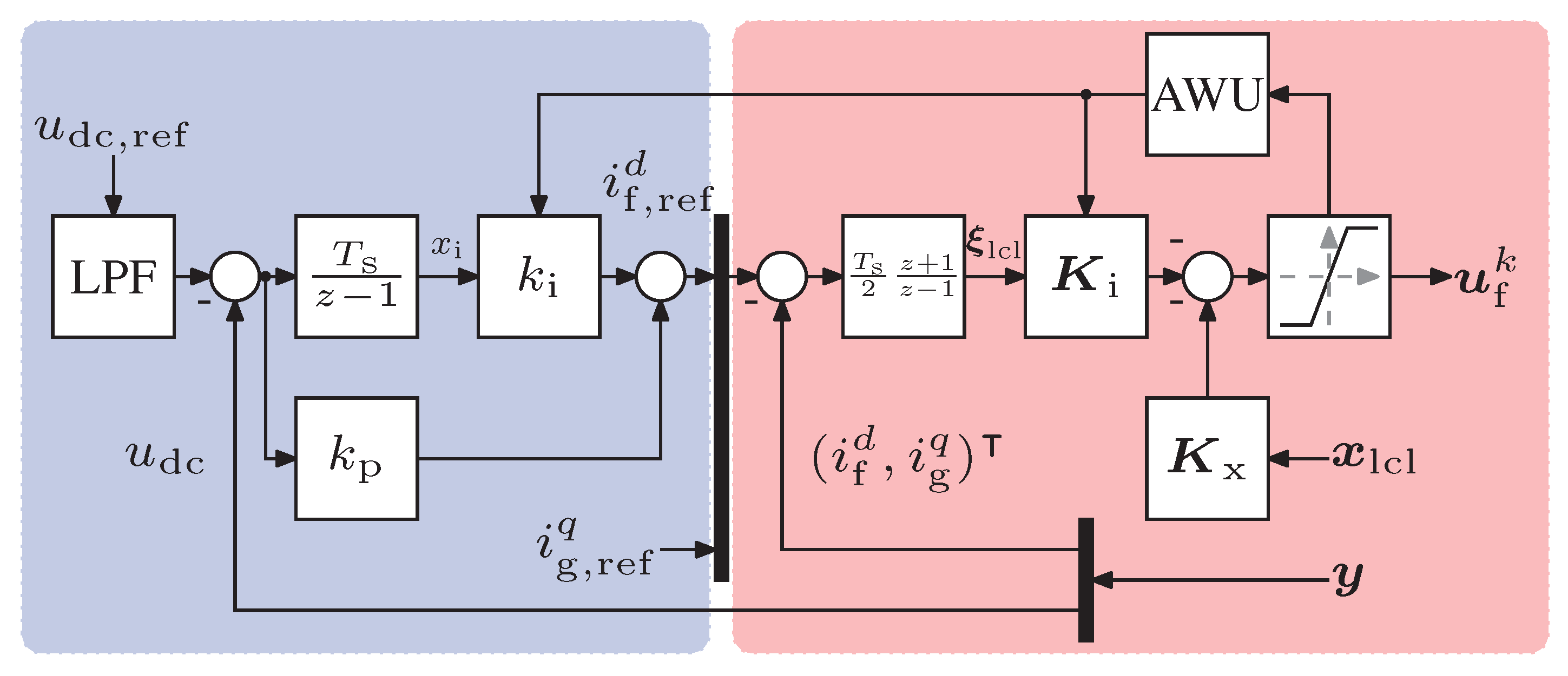
3. Dlqr Current Controller with Integral Feedback

The chosen method for controlling the filter current ${\mathit{i}}_{\mathrm{f}}^{dq}$ is a discrete-time linear-quadratic regulator design. The proposed current controller is based on [42]. As mentioned in [48], a LQR controller shows a better dynamic performance and a greater robustness against parameter uncertainties and nonlinearities—as present in the case of the nonlinear dc-link voltage dynamics. A successful LQR controller design is linked to several requirements ([49], Chap. 12):

(i)

the system must be completely controllable $[{\mathit{A}}_{\mathrm{lcl}},{\mathit{B}}_{\mathrm{lcl}}]$ and observable $[{\mathit{A}}_{\mathrm{lcl}},{\mathit{C}}_{\mathrm{lcl}}]$,

(ii)

the weighting matrices ${\mathit{Q}}_{\mathrm{lcl}}\in {\mathbb{R}}^{8\times 8}$ and ${\mathit{R}}_{\mathrm{lcl}}\in {\mathbb{R}}^{2\times 2}$ must be symmetrical and positive semi-definite and positive definite, respectively, and

(iii)

the system $[{\mathit{A}}_{\mathrm{lcl}},{\mathit{Q}}_{\mathrm{lcl}}]$ must be observable.

Choosing the d-component of the GCI output current $i_{\mathrm{f}}^d$ and the q-component of the grid current $i_{\mathrm{g}}^q$ as system outputs leads to the following output equation

$$\begin{array}{c}\hfill {\mathit{y}}_{\mathrm{lcl}}\left(t\right)={(i_{\mathrm{f}}^d,i_{\mathrm{g}}^q)}^{\top }=\underset{{\mathit{C}}_{\mathrm{lcl}}\in {\mathbb{R}}^{2\times 6}}{\underbrace{\left[\begin{array}{cccccc}1& 0& 0& 0& 0& 0\\ 0& 0& 0& 1& 0& 0\end{array}\right]}}{\mathit{x}}_{\mathrm{lcl}}\left(t\right).\end{array}$$

In order to prevent steady-state errors, additional integrators need to be implemented in the control loop. This leads to an augmented LCL filter state-space model (2) with additional states ${\mathsf{\xi }}_{\mathrm{lcl}}\in {\mathbb{R}}^2$ of the integrators. The augmented system is given by

$$\begin{array}{c}\hfill \frac{\mathrm{d}}{\mathrm{d}t}\left(\begin{array}{c}{\mathit{x}}_{\mathrm{lcl}}\left(t\right)\\ {\mathsf{\xi }}_{\mathrm{lcl}}\left(t\right)\end{array}\right)=\stackrel{:={\mathit{A}}_{\mathsf{\xi }}\in {\mathbb{R}}^{8\times 8}}{\overbrace{\left[\begin{array}{cc}{\mathit{A}}_{\mathrm{lcl}}& {\mathit{O}}_{6\times 2}\\ -{\mathit{C}}_{\mathrm{lcl}}& {\mathit{O}}_{2\times 2}\end{array}\right]}}\stackrel{:={\mathit{z}}_{\mathrm{lcl}}}{\overbrace{\left(\begin{array}{c}{\mathit{x}}_{\mathrm{lcl}}\left(t\right)\\ {\mathsf{\xi }}_{\mathrm{lcl}}\left(t\right)\end{array}\right)}}+\stackrel{:={\mathit{G}}_{\mathsf{\xi }}\in {\mathbb{R}}^{8\times 2}}{\overbrace{\left[\begin{array}{c}{\mathit{O}}_{6\times 2}\\ {\mathit{I}}_2\end{array}\right]}}\left(\begin{array}{c}{i}_{\mathrm{f},\mathrm{ref}}^d\left(t\right)\\ i_{\mathrm{g},\mathrm{ref}}^q\left(t\right)\end{array}\right)+\underset{:={\mathit{B}}_{\mathsf{\xi }}\in {\mathbb{R}}^{8\times 2}}{\underbrace{{\left[\begin{array}{cc}{\mathit{B}}_{\mathrm{lcl}}^{\top }& {\mathit{O}}_{2\times 2}\end{array}\right]}^{\top }}}{\mathit{u}}_{\mathrm{f}}^{dq}\left(t\right),\end{array}$$

With the augmented system state ${\mathit{z}}_{\mathrm{lcl}}:={({\mathit{x}}_{\mathrm{lcl}}^{\top },{\mathsf{\xi }}_{\mathrm{lcl}}^{\top })}^{\top }$ and the augmented matrices ${\mathit{A}}_{\mathsf{\xi }}$ and ${\mathit{B}}_{\mathsf{\xi }}$, ${\mathit{G}}_{\mathsf{\xi }}$. Because of the low sampling frequency $f_{\mathrm{s}}$, a continuous-time linear-quadratic controller design would lead to an unstable system behavior, as illustrated in Figure 3. Remedy provides a system discretization by the step invariant method as described in [50,51] and a discrete-time linear-quadratic optimization. Applying the discretization rules and choosing the approximation factor $N=8$, which is a numerically reasonable choice [50], leads to the equivalent discrete-time matrices

$$\begin{array}{c}{\mathit{S}}_{\mathrm{lcl}}=T_{\mathrm{s}}\sum _{\nu =0}^{N=8}{\mathit{A}}_{\mathsf{\xi }}^{\nu }\frac{T_{\mathrm{s}}^{\nu }}{(\nu +1)!}\mathrm{with}\hfill \\ {\mathit{A}}_{\mathrm{k}\mathsf{\xi }}={\mathit{I}}_8+{\mathit{S}}_{\mathrm{lcl}}{\mathit{A}}_{\mathsf{\xi }},{\mathit{B}}_{\mathrm{k}\mathsf{\xi }}={\mathit{S}}_{\mathrm{lcl}}{\mathit{B}}_{\mathsf{\xi }},{\mathit{G}}_{\mathrm{k}\mathsf{\xi }}={\mathit{S}}_{\mathrm{lcl}}{\mathit{G}}_{\mathsf{\xi }}\hfill \end{array}\}$$

(5)

and the discrete-time system dynamics

$$\begin{array}{c}\hfill \begin{array}{cc}\hfill \left(\begin{array}{c}{\mathit{x}}_{\mathrm{lcl}}[k+1]\\ {\mathsf{\xi }}_{\mathrm{lcl}}[k+1]\end{array}\right)=& {\mathit{A}}_{\mathrm{k}\mathsf{\xi }}\left(\begin{array}{c}{\mathit{x}}_{\mathrm{lcl}}\left[k\right]\\ {\mathsf{\xi }}_{\mathrm{lcl}}\left[k\right]\end{array}\right)+{\mathit{B}}_{\mathrm{k}\mathsf{\xi }}{\mathit{u}}_{\mathrm{f}}^{dq}\left[k\right]+{\mathit{G}}_{\mathrm{k}\mathsf{\xi }}\left(\begin{array}{c}{i}_{\mathrm{f},\mathrm{ref}}^d\left[k\right]\\ i_{\mathrm{g},\mathrm{ref}}^q\left[k\right]\end{array}\right).\hfill \end{array}\end{array}$$

(6)

The (discrete) LQ optimization is performed according to ([49], Chap. 12–13) and ([52], Chap. 6), where a detailed description of this method can be found. In general, the aim of the LQR design is to minimize a cost function; here, the cost function is chosen as

$$\begin{array}{c}\hfill J({\mathit{z}}_{\mathrm{lcl}},{\mathit{u}}_{\mathrm{f}}^{dq})=\sum _{k=0}^{\infty }({\mathit{z}}_{\mathrm{lcl}}{\left[k\right]}^{\top }{\mathit{Q}}_{\mathrm{lcl}}{\mathit{z}}_{\mathrm{lcl}}\left[k\right]+{\mathit{u}}_{\mathrm{f}}^{dq}{\left[k\right]}^{\top }{\mathit{R}}_{\mathrm{lcl}}{\mathit{u}}_{\mathrm{f}}^{dq}\left[k\right]).\end{array}$$

Its minimization is subject to an equality constraint (system dynamics) and it can be formulated as

$$\begin{array}{c}\hfill \underset{{\mathit{u}}_{\mathrm{f}}^{dq}}{min}J({\mathit{z}}_{\mathrm{lcl}},{\mathit{u}}_{\mathrm{f}}^{dq})\mathrm{such}\mathrm{that}{\mathit{z}}_{\mathrm{lcl}}[k+1]={\mathit{A}}_{\mathrm{k}\mathsf{\xi }}{\mathit{z}}_{\mathrm{lcl}}\left[k\right]+{\mathit{B}}_{\mathrm{k}\mathsf{\xi }}{\mathit{u}}_{\mathrm{f}}^{dq}\left[k\right].\end{array}$$

This optimization problem can be transferred to an equivalent (dual) problem without constraint by introducing the Hamilton function

$$\begin{array}{c}\hfill H({\mathit{z}}_{\mathrm{lcl}},{\mathit{u}}_{\mathrm{f}}^{dq},\mathrm{\Lambda })=\frac{1}{2}\left({\mathit{z}}_{\mathrm{lcl}}{\left[k\right]}^{\top }{\mathit{Q}}_{\mathrm{lcl}}{\mathit{z}}_{\mathrm{lcl}}\left[k\right]\right)+\frac{1}{2}\left({\mathit{u}}_{\mathrm{f}}^{dq}{\left[k\right]}^{\top }{\mathit{R}}_{\mathrm{lcl}}{\mathit{u}}_{\mathrm{f}}^{dq}\left[k\right]\right)+\mathrm{\Lambda }{[k+1]}^{\top }({\mathit{A}}_{\mathrm{k}\mathsf{\xi }}{\mathit{z}}_{\mathrm{lcl}}\left[k\right]+{\mathit{B}}_{\mathrm{k}\mathsf{\xi }}{\mathit{u}}_{\mathrm{f}}^{dq}\left[k\right])\end{array}$$

(7)

and the Lagrange multiplier

$$\begin{array}{c}\hfill \mathrm{\Lambda }\left[k\right]=\mathit{P}{\mathit{z}}_{\mathrm{lcl}}\left[k\right].\end{array}$$

The optimality conditions for the global minimum of the Hamilton function (7) yield the Ricatti difference equation

$$\begin{array}{c}\hfill {\mathit{Q}}_{\mathrm{lcl}}-\mathit{P}+{\mathit{A}}_{\mathrm{k}\mathsf{\xi }}^{\top }\mathit{P}{\mathit{A}}_{\mathrm{k}\mathsf{\xi }}-{\mathit{A}}_{\mathrm{k}\mathsf{\xi }}^{\top }\mathit{P}{\mathit{B}}_{\mathrm{k}\mathsf{\xi }}{({\mathit{R}}_{\mathrm{lcl}}+{\mathit{B}}_{\mathrm{k}\mathsf{\xi }}^{\top }\mathit{P}{\mathit{B}}_{\mathrm{k}\mathsf{\xi }})}^{-1}{\mathit{B}}_{\mathrm{k}\mathsf{\xi }}\mathit{P}{\mathit{A}}_{\mathrm{k}\mathsf{\xi }}={\mathit{O}}_{8\times 8},\end{array}$$

(8)

which must be solved for some symmetric and positive definite matrix $\mathit{P}={\mathit{P}}^{\top }>0$ and results in the DLQR control law

$$\begin{array}{cc}\hfill {\mathit{u}}_{\mathrm{f}}^{dq}\left[k\right]& =-\underset{:=\left[\begin{array}{cc}{\mathit{K}}_{\mathrm{x}}& {\mathit{K}}_{\mathrm{i}}\end{array}\right]}{\underbrace{{({\mathit{R}}_{\mathrm{lcl}}+{\mathit{B}}_{\mathrm{k}\mathsf{\xi }}^{\top }\mathit{P}{\mathit{B}}_{\mathrm{k}\mathsf{\xi }})}^{-1}{\mathit{B}}_{\mathrm{k}\mathsf{\xi }}\mathit{P}{\mathit{A}}_{\mathrm{k}\mathsf{\xi }}}}{\mathit{z}}_{\mathrm{lcl}}\left[k\right]=-{\mathit{K}}_{\mathrm{x}}{\mathit{x}}_{\mathrm{lcl}}\left[k\right]-{\mathit{K}}_{\mathrm{i}}{\mathsf{\xi }}_{\mathrm{lcl}}\left[k\right],\hfill \end{array}$$

(9)

where ${\mathit{K}}_{\mathrm{x}}\in {\mathbb{R}}^{2\times 6}$ and ${\mathit{K}}_{\mathrm{i}}\in {\mathbb{R}}^{2\times 2}$ are the feedback matrices, which stabilize the closed-loop system.

The weighting matrices

$$\begin{array}{c}\hfill {\mathit{Q}}_{\mathrm{lcl}}=diag\left({\mathbf{1}}_2^{\top }\frac{q_{\mathrm{if}}}{q_{\mathrm{if},\mathrm{m}}^2},{\mathbf{1}}_2^{\top }\frac{q_{\mathrm{ig}}}{q_{\mathrm{ig},\mathrm{m}}^2},{\mathbf{1}}_2^{\top }\frac{q_{\mathrm{uc}}}{q_{\mathrm{uc},\mathrm{m}}^2},{\mathbf{1}}_2^{\top }\frac{q_{\mathsf{\xi }}}{q_{\mathsf{\xi },\mathrm{m}}^2}\right)\mathrm{and}{\mathit{R}}_{\mathrm{lcl}}=diag\left({\mathbf{1}}_2^{\top }\frac{q_{\mathrm{uf}}}{q_{\mathrm{uf},\mathrm{m}}^2}\right)\end{array}$$

(10)

incorporate the tuning parameters of the LQR design and have a significant impact on the behavior of the closed-loop system. In the literature, there is no straight forward method given for an optimal choice of this matrices. The Bryson method is a heuristic and often used approach [53]. The weighting matrices are chosen as diagonal matrices, and each diagonal element is normalized by its squared maximum value. This allows to achieve an equal impact of each state $z_{\mathrm{lcl},\mathrm{i}}$ on the cost function. After normalization, it is a gradual process to find the “best” control performance of the closed-loop system by tuning the weights individually. This can be done by varying the numerator coefficients in (10).

The chosen weights are listed in

Table 3. Values of weighting factors.

$\frac{{\mathit{q}}_{\mathbf{if}}}{{\mathit{q}}_{\mathbf{if},\mathbf{m}}^2}$	$\frac{{\mathit{q}}_{\mathbf{ig}}}{{\mathit{q}}_{\mathbf{ig},\mathbf{m}}^2}$	$\frac{{\mathit{q}}_{\mathbf{uc}}}{{\mathit{q}}_{\mathbf{uc},\mathbf{m}}^2}$	$\frac{{\mathit{q}}_{\mathsf{\xi }}}{{\mathit{q}}_{\mathsf{\xi },\mathbf{m}}^2}$	$\frac{{\mathit{r}}_{\mathbf{uf}}}{{\mathit{r}}_{\mathbf{uf},\mathbf{m}}^2}$	N	${\mathit{k}}_{\mathbf{p}}$	${\mathit{k}}_{\mathbf{i}}$
$\frac{1}{{30}^2}$	$\frac{1}{{30}^2}$	$\frac{1}{2·{230}^2}$	$\frac{10}{0.{025}^2}$	$\frac{1}{2·{230}^2}$	8	$-0.1$	$-15$

. Special attention is needed for the choice of factor $q_{\mathsf{\xi }}$. This factor weights the integral error of the current controller and has a great impact on the controller’s performance and, therefore, the cascaded dc-link controller.

The optimization (i.e., solving the Riccati difference equation in (8)) was done in Matlab/Simulink R2017b (MathWorks, Natick, Massachusetts, USA) using the integrated function dlqr() which returns the feedback matrices ${\mathit{K}}_{\mathrm{x}}$ and ${\mathit{K}}_{\mathrm{i}}$. Since the output voltage ${\mathit{u}}_{\mathrm{f}}^{dq}$ of the GCI is limited, an additional saturation and anti-windup strategy is implemented ([44] Chap. 14).

Figure 4 shows the simulation results of the discrete-time implementation of the current controller. The used solver was ode4 with a fixed time-step of $t_{\mathrm{step}}=2.5 \mathsf{\mu }\mathrm{s}$. It can be seen that all system states are stable during the whole simulation. The controller has a good performance and follows the reference steps of $\pm 20 \mathrm{A}$ within 2 $\mathrm{m}$$\mathrm{s}$.

4. Dc-Link Voltage Controller

Figure 5 shows the overall and cascaded controller structure. The current state-feedback controller is highlighted in red; the dc-link voltage PI controller is highlighted in blue.

4.1. Derivation of Closed-Loop System

The overall controller design is based on the small-signal approximation (2) and (4), which are merged to the overall linearized system dynamics

$$\begin{array}{c}\hfill \frac{\mathrm{d}}{\mathrm{d}t}\stackrel{:={\tilde{\mathit{x}}}_{\mathrm{d}}\in {\mathbb{R}}^7}{\overbrace{\left(\begin{array}{c}{\tilde{\mathit{x}}}_{\mathrm{lcl}}\left(t\right)\\ {\tilde{u}}_{\mathrm{dc}}\left(t\right)\end{array}\right)}}=\stackrel{:={\mathit{A}}_{\mathrm{d}}^{🟉}\in {\mathbb{R}}^{7\times 7}}{\overbrace{\left[\begin{array}{cc}{\mathit{A}}_{\mathrm{lcl}}& {\mathbf{0}}_6\\ {\left({\mathit{a}}_{\mathrm{dc}}^{🟉}\right)}^{\top }& 0\end{array}\right]}}\left(\begin{array}{c}{\tilde{\mathit{x}}}_{\mathrm{lcl}}\left(t\right)\\ {\tilde{u}}_{\mathrm{dc}}\left(t\right)\end{array}\right)+\stackrel{:={\mathit{B}}_{\mathrm{d}}^{🟉}\in {\mathbb{R}}^{7\times 2}}{\overbrace{\left[\begin{array}{c}{\mathit{B}}_{\mathrm{lcl}}\\ {\left({\mathit{b}}_{\mathrm{dc}}^{🟉}\right)}^{\top }\end{array}\right]}}{\tilde{\mathit{u}}}_{\mathrm{f}}^{dq}\left(t\right)+\underset{:={\mathit{E}}_{\mathrm{d}}^{🟉}\in {\mathbb{R}}^{7\times 3}}{\underbrace{\left[\begin{array}{cc}{\mathit{E}}_{\mathrm{lcl}}& {\mathbf{0}}_6\\ {\mathbf{0}}_2^{\top }& \frac{1}{C_{\mathrm{dc}}{u}_{\mathrm{dc}}^{🟉}}\end{array}\right]}}\underset{:={\tilde{\mathit{d}}}_{\mathrm{d}}\in {\mathbb{R}}^3}{\underbrace{\left(\begin{array}{c}{\tilde{\mathit{d}}}_{\mathrm{lcl}}\left(t\right)\\ {\tilde{p}}_{\mathrm{m}}\left(t\right)\end{array}\right)}}.\end{array}$$

(11)

The small-signal dynamics in (2) do not change due to their linearity. Applying the discretization method, as in (5) to (11), yields

$$\begin{array}{c}\begin{array}{c}{\mathit{S}}_{\mathrm{d}}=T_{\mathrm{s}}\sum _{\nu =0}^8{\left({\mathit{A}}_{\mathrm{d}}^{🟉}\right)}^{\nu }\frac{T_{\mathrm{s}}^{\nu }}{(\nu +1)!}\hfill \end{array}\hfill \\ {\mathit{A}}_{\mathrm{k}\mathrm{d}}^{🟉}={\mathit{I}}_7+{\mathit{S}}_{\mathrm{d}}{\mathit{A}}_{\mathrm{d}}^{🟉},{\mathit{B}}_{\mathrm{k}\mathrm{d}}^{🟉}={\mathit{S}}_{\mathrm{d}}{\mathit{B}}_{\mathrm{d}}^{🟉},{\mathit{E}}_{\mathrm{k}\mathrm{d}}^{🟉}={\mathit{S}}_{\mathrm{d}}{\mathit{E}}_{\mathrm{d}}^{🟉}\hfill \end{array}\}$$

and gives the discrete-time LTI small-signal dynamics

$$\begin{array}{cc}{\tilde{\mathit{x}}}_{\mathrm{d}}[k+1]\hfill & ={\mathit{A}}_{\mathrm{k}\mathrm{d}}^{🟉}{\tilde{\mathit{x}}}_{\mathrm{d}}\left[k\right]+{\mathit{B}}_{\mathrm{k}\mathrm{d}}^{🟉}{\tilde{\mathit{u}}}_{\mathrm{f}}^{dq}\left[k\right]+{\mathit{E}}_{\mathrm{k}\mathrm{d}}^{🟉}{\tilde{\mathit{d}}}_{\mathrm{d}}\left[k\right]\\ {\tilde{u}}_{\mathrm{dc}}\left[k\right]\hfill & =\underset{:={\mathit{c}}_{\chi }^{\top }\in {\mathbb{R}}^7}{\underbrace{\left[\begin{array}{ccccccc}0& 0& 0& 0& 0& 0& 1\end{array}\right]}}{\tilde{\mathit{x}}}_{\mathrm{d}}\left[k\right]\hfill \end{array}\}$$

(12)

In view of the inner current control loop, as described in Section 3, the integrator states ${\mathsf{\xi }}_{\mathrm{lcl}}$ and ${\tilde{\mathsf{\xi }}}_{\mathrm{lcl}}$, respectively, need to also be considered in (12). The current controller uses the more accurate trapezoidal discretization method for the integrator, as given by

$$\begin{array}{c}\hfill {\tilde{\mathsf{\xi }}}_{\mathrm{lcl}}[k+1]={\tilde{\mathsf{\xi }}}_{\mathrm{lcl}}\left[k\right]+\frac{T_{\mathrm{s}}}{2}\left(\left(\begin{array}{c}{\tilde{i}}_{\mathrm{f},\mathrm{ref}}^d[k+1]\\ {\tilde{i}}_{\mathrm{g},\mathrm{ref}}^q[k+1]\end{array}\right)+\left(\begin{array}{c}{\tilde{i}}_{\mathrm{f},\mathrm{ref}}^d\left[k\right]\\ {\tilde{i}}_{\mathrm{g},\mathrm{ref}}^q\left[k\right]\end{array}\right)-\underset{:={\mathit{C}}_{\mathrm{k}\mathrm{d}}^{🟉}}{\underbrace{\left[\begin{array}{cc}{\mathit{C}}_{\mathrm{lcl}}& {\mathbf{0}}_2\end{array}\right]}}{\tilde{\mathit{x}}}_{\mathrm{d}}\left[k\right]\right).\end{array}$$

(13)

Merging (12) and (13) leads to the overall discrete-time system description

$$\begin{array}{c}\hfill \begin{array}{cc}\hfill \stackrel{:={\tilde{\mathit{x}}}_{\chi }[k+1]\in {\mathbb{R}}^9}{\overbrace{\left(\begin{array}{c}{\tilde{\mathit{x}}}_{\mathrm{d}}[k+1]\\ {\tilde{\mathsf{\xi }}}_{\mathrm{lcl}}[k+1]\end{array}\right)}}=& \stackrel{:={\mathit{A}}_{\chi }^{🟉}\in {\mathbb{R}}^{9\times 9}}{\overbrace{\left[\begin{array}{cc}{\mathit{A}}_{\mathrm{k}\mathrm{d}}^{🟉}& {\mathit{O}}_{7\times 2}\\ -\frac{T_{\mathrm{s}}}{2}{\mathit{C}}_{\mathrm{k}\mathrm{d}}^{🟉}({\mathit{A}}_{\mathrm{k}\mathrm{d}}^{🟉}+{\mathit{I}}_7)& {\mathit{I}}_2\end{array}\right]}}\left(\begin{array}{c}{\tilde{\mathit{x}}}_{\mathrm{d}}\left[k\right]\\ {\tilde{\mathsf{\xi }}}_{\mathrm{lcl}}\left[k\right]\end{array}\right)\hfill \\ \hfill & +\underset{:={\mathit{B}}_{\chi }^{🟉}\in {\mathbb{R}}^{9\times 2}}{\underbrace{\left[\begin{array}{c}{\mathit{B}}_{\mathrm{k}\mathrm{d}}^{🟉}\\ -\frac{T_{\mathrm{s}}}{2}{\mathit{C}}_{\mathrm{k}\mathrm{d}}^{🟉}{\mathit{B}}_{\mathrm{k}\mathrm{d}}^{🟉}\end{array}\right]}}{\tilde{\mathit{u}}}_{\mathrm{f}}^{dq}\left[k\right]+\underset{:={\mathit{E}}_{\chi }^{🟉}\in {\mathbb{R}}^{9\times 3}}{\underbrace{\left[\begin{array}{cc}{\mathit{e}}_{\mathrm{d}}^{🟉}& {\mathit{O}}_{8\times 2}\\ -\frac{T_{\mathrm{s}}}{2}{\mathit{C}}_{\mathrm{k}\mathrm{d}}^{🟉}{\mathit{e}}_{\mathrm{d}}^{🟉}& \frac{T_{\mathrm{s}}}{2}{\mathbf{1}}_2^{\top }\end{array}\right]}}\underset{:={\tilde{\mathit{d}}}_{\chi }[k+1]\in {\mathbb{R}}^3}{\underbrace{\left(\begin{array}{c}{\tilde{p}}_{\mathrm{m}}\left[k\right]\\ {\tilde{i}}_{\mathrm{g},\mathrm{ref}}^q\left[k\right]\\ {\tilde{i}}_{\mathrm{g},\mathrm{ref}}^q[k+1]\end{array}\right)}}\hfill \\ \hfill & +{\left(\begin{array}{ccc}{\mathbf{0}}_7^{\top }& \frac{T_{\mathrm{s}}}{2}& 0\end{array}\right)}^{\top }\left({\tilde{i}}_{\mathrm{f},\mathrm{ref}}^d\left[k\right]+{\tilde{i}}_{\mathrm{f},\mathrm{ref}}^d[k+1]\right).\hfill \end{array}\end{array}$$

(14)

The control law in (9) now becomes

$$\begin{array}{c}\hfill {\tilde{\mathit{u}}}_{\mathrm{f}}^{dq}\left[k\right]=-\underset{:={\mathit{K}}_{\chi }}{\underbrace{\left[\begin{array}{ccc}{\mathit{K}}_{\mathrm{x}}& {\mathbf{0}}_2& {\mathit{K}}_{\mathrm{i}}\end{array}\right]}}{\tilde{\mathit{x}}}_{\chi }\left[k\right]\end{array}$$

and it can be applied to (14). As illustrated in Figure 5, the integrator used for the dc-link voltage controller

$$\begin{array}{c}\hfill {\tilde{x}}_i[k+1]={\tilde{x}}_i\left[k\right]+T_{\mathrm{s}}\left({\tilde{u}}_{\mathrm{dc},\mathrm{ref}}\left[k\right]-{\tilde{u}}_{\mathrm{dc}}\left[k\right]\right)\end{array}$$

(15)

is implemented by a simple Forward Euler (FE) discretization in view of an easier stability analysis in combination with the integrator state ${\tilde{x}}_i\in \mathbb{R}$, which also needs to be merged with (14). In contrast, the current control loop has a trapezoidal integrator (see Figure 5). Actually, in order to be mathematically correct, an integrator of order $N=8$ should be used, but, since the trapezoidal integrator has the highest available order in MATLAB, it was used for the current controller design. For (14) and (15), the dc-link PI control law is finally given by

$$\begin{array}{c}\hfill {\tilde{i}}_{\mathrm{f},\mathrm{ref}}^d\left[k\right]=k_{\mathrm{i}}{\tilde{\mathit{x}}}_{\chi }\left[k\right]+k_{\mathrm{p}}\left({\tilde{u}}_{\mathrm{dc},\mathrm{ref}}\left[k\right]-{\tilde{u}}_{\mathrm{dc}}\left[k\right]\right)\end{array}$$

(16)

and, due to the trapezoidal integrator (13) of the state-feedback current controller, the control law for the feed-through term becomes

$$\begin{array}{cc}\hfill & {\tilde{i}}_{\mathrm{f},\mathrm{ref}}^d[k+1]=k_{\mathrm{i}}{\tilde{x}}_i\left[k\right]+k_{\mathrm{i}}{T}_{\mathrm{s}}{\tilde{u}}_{\mathrm{dc},\mathrm{ref}}\left[k\right]-k_{\mathrm{i}}{T}_{\mathrm{s}}{\mathbf{c}}_{\chi }^{\top }{\tilde{\mathit{x}}}_{\mathrm{d}}\left[k\right]\hfill \\ \hfill & +k_{\mathrm{p}}{\tilde{u}}_{\mathrm{dc},\mathrm{ref}}[k+1]-k_{\mathrm{p}}{\mathit{c}}_{\chi }^{\top }\left({\mathit{A}}_{\mathrm{k}\mathrm{d}}^{🟉}{\tilde{\mathit{x}}}_{\mathrm{d}}\left[k\right]+{\mathit{B}}_{\mathrm{k}\mathrm{d}}^{🟉}{\mathit{u}}_{\mathrm{f}}^{dq}\left[k\right]+{\mathit{e}}_{\mathrm{d}}^{🟉}{\tilde{p}}_{\mathrm{m}}\left[k\right]\right).\hfill \end{array}$$

(17)

By adding the control laws (16) and (17), the term ${\tilde{i}}_{\mathrm{f},\mathrm{ref}}^d\left[k\right]+{\tilde{i}}_{\mathrm{f},\mathrm{ref}}^d[k+1]$ in (14) can be replaced by

$$\begin{array}{c}\hfill \begin{array}{cc}\hfill {\tilde{i}}_{\mathrm{f},\mathrm{ref}}^d\left[k\right]+{\tilde{i}}_{\mathrm{f},\mathrm{ref}}^d[k+1]=& 2k_{\mathrm{i}}{\tilde{x}}_i\left[k\right]+(k_{\mathrm{p}}+k_{\mathrm{i}}{T}_{\mathrm{s}}){\tilde{u}}_{\mathrm{dc},\mathrm{ref}}\left[k\right]\hfill \\ \hfill & +k_{\mathrm{p}}{\tilde{u}}_{\mathrm{dc},\mathrm{ref}}[k+1]-k_{\mathrm{p}}{\mathit{c}}_{\chi }^{\top }{\mathit{e}}_{\mathrm{d}}^{🟉}{\tilde{p}}_{\mathrm{m}}\left[k\right]\hfill \\ \hfill & +\underset{:={\left({\mathbf{a}}_{\chi }^{🟉}\right)}^{\top }\in {\mathbb{R}}^9}{\underbrace{\left(k_{\mathrm{p}}{\mathit{c}}_{\chi }^{\top }{\mathit{B}}_{\mathrm{k}\mathrm{d}}^{🟉}{\mathit{K}}_{\chi }-\left(\begin{array}{cc}{k}_{\mathrm{p}}{\mathit{c}}_{\chi }^{\top }({\mathit{I}}_7+{\mathit{A}}_{\mathrm{k}\mathrm{d}}^{🟉})+k_{\mathrm{i}}{T}_{\mathrm{s}}{\mathbf{c}}_{\chi }^{\top }& {\mathbf{0}}_2^{\top }\end{array}\right)\right)}}{\tilde{\mathbf{x}}}_{\chi }\left[k\right],\hfill \end{array}\end{array}$$

which leads together with the FE integrator (15) to the overall closed-loop system dynamics

$$\begin{array}{c}\hfill \begin{array}{cc}\hfill \left(\begin{array}{c}{\tilde{\mathit{x}}}_{\chi }[k+1]\\ {\tilde{x}}_i[k+1]\end{array}\right)=& \stackrel{:={\mathit{A}}_{\mathrm{cl}}^{🟉}\in {\mathbb{R}}^{10\times 10}}{\overbrace{\left[\begin{array}{cc}{\mathit{A}}_{\chi }^{🟉}-{\mathit{B}}_{\chi }^{🟉}{\mathit{K}}_{\chi }+{\mathit{b}}_{\chi }{\left({\mathit{a}}_{\chi }^{🟉}\right)}^{\top }& 2k_{\mathrm{i}}{\mathit{b}}_{\chi }\\ \left[\begin{array}{cc}-T_{\mathrm{s}}{\mathit{c}}_{\chi }^{\top }& {\mathbf{0}}_2^{\top }\end{array}\right]& 1\end{array}\right]}}\left(\begin{array}{c}{\tilde{\mathit{x}}}_{\chi }\left[k\right]\\ {\tilde{x}}_i\left[k\right]\end{array}\right)\hfill \\ \hfill & +\left[\begin{array}{cc}(k_{\mathrm{p}}+k_{\mathrm{i}}{T}_{\mathrm{s}}){\mathit{b}}_{\chi }& k_{\mathrm{p}}{\mathit{b}}_{\chi }\\ T_{\mathrm{s}}& 0\end{array}\right]\left(\begin{array}{c}{\tilde{u}}_{\mathrm{dc},\mathrm{ref}}\left[k\right]\\ {\tilde{u}}_{\mathrm{dc},\mathrm{ref}}[k+1]\end{array}\right)\hfill \\ \hfill & +\left[\begin{array}{c}{\mathit{E}}_{\chi }^{🟉}-k_{\mathrm{p}}{\mathit{b}}_{\chi }{\mathit{c}}_{\chi }^{\top }{\mathit{e}}_{\mathrm{d}}^{🟉}\left(\begin{array}{ccc}1& 0& 0\end{array}\right)\\ {\mathbf{0}}_3^{\top }\end{array}\right]{\tilde{\mathit{d}}}_{\chi }[k+1].\hfill \end{array}\end{array}$$

(18)

4.2. Stability Analysis of Closed-Loop System

System stability is analyzed based on the small-signal dynamics (18) of the closed loop system (Note that the presented discussion does not cover a large-signal stability analysis as only the linearized (small-signal) system dynamics are analyzed. In order to discuss and analyze global stability, the overall nonlinear system dynamics (2)+(3) need to be studied by e.g., Lyapunov’s method ([54], [Chap. 3])). Because no dc-link voltage reference jumps or load jumps usually occur, the local analysis is sufficient. Moreover, to guarantee system stability over the whole operating range, several operating points close to the instability boundary are chosen (see Figure 6). The theoretical analysis yields controller parameter sets to ensure local stability for each operating point. The controller parameters are chosen from the most limiting parameter set assigned to the worst-case operating scenario.

To locally analyze the stability of the system, its matrix ${\mathbf{A}}_{\mathrm{cl}}^{🟉}$ is investigated. The system is locally asymptotically stable if all eigenvalues $|{\mathit{\lambda }}_{k,i}|<1$, $i=1,..,10$ are within the unit circle of the complex plane. Because the system was linearized, the whole operating range needs to be considered to guarantee in each point local system stability.

Table 4. relevant operating points for sampling frequency $f_{\mathrm{s}}=4\mathrm{kHz}$ and weighting factor $q_{\xi }=10$.

OP	${\mathit{i}}_{\mathbf{f}}^{\mathit{d}🟉}$ / $\mathbf{A}$	${\mathit{i}}_{\mathbf{g}}^{\mathit{q}🟉}$ / $\mathbf{A}$	${\mathit{u}}_{\mathbf{dc}}^{🟉}$ / $\mathbf{V}$	${\mathit{u}}_{\mathbf{f}}^{\mathit{d}🟉}$ / $\mathbf{V}$	${\mathit{u}}_{\mathbf{f}}^{\mathit{q}🟉}$ / $\mathbf{V}$
OP1	0	0	750	324.47	0.1
OP2	0	0	600	324.47	0.1
OP3	0	0	900	324.47	0.1
OP4	−11.5	0	750	321.01	−25.26
OP5	11.5	0	750	327.92	25.47
OP6	0	−11.5	750	349.71	−3.35
OP7	0	11.5	750	299.22	3.56
OP8	−11.5	−11.5	600	346.26	−28.72
OP9	−11.5	11.5	600	295.76	−21.81

shows all of the investigated operating points (OPs), which span over the whole operating range of the considered system. OP1 is defined as reference point. Figure 6 illustrates the impact of (a) $u_{\mathrm{dc}}^{🟉}$, (b) $i_{\mathrm{f}}^{d🟉}$, (c) $i_{\mathrm{g}}^{q🟉}$, (d) $f_{\mathrm{s}}$, (e) $q_{\xi }$ on the stabilizing PI controller parameters $k_{\mathrm{p}}$ (in $\frac{\mathrm{A}}{\mathrm{V}}$) and $k_{\mathrm{i}}$ (in $\frac{\mathrm{A}}{\mathrm{V}\mathrm{s}}$). It can be seen that the filter current $i_{\mathrm{f}}^{d🟉}$ has the greatest impact on the stability region (see Figure 6b). The smaller (or more negative) the current $i_{\mathrm{f}}^{d🟉}$, the smaller the stability region. The dc-link voltage $u_{\mathrm{dc}}^{🟉}$ (see Figure 6a) also has a high impact. The stability region shrinks with decreasing voltage $u_{\mathrm{dc}}^{🟉}$. Almost negligible is the impact of grid current $i_{\mathrm{g}}^{q🟉}$ on the controller parameter tuning (see Figure 6c). A variation of the sampling frequency $f_{\mathrm{s}}$ is shown in Figure 6d. Its impact is obvious. A high sampling frequency ensures a larger stability region and allows, therefore, for a quasi-continuous controller design. The stability region decreases with decreasing sampling frequency.

Figure 6e shows the impact of the current controller performance on the stability region. As mentioned in Section 3 this parameter has a significant impact on the PI controller parameters. A larger weighting factor $q_{\xi }$ leads to a faster current control system and, thus, a larger stability region. Combining the knowledge of the impact of each variable from Figure 6 leads to the worst case scenario operating point (OP9 in Table 4), which is shown in Figure 7a. On basis of this plot, the final controller parameters are obtained.

The choice of the controller’s parameters is a compromise. A high proportional factor $k_{\mathrm{p}}$ of the dc-link controller is desirable to respond quickly to any disturbances acting on the system. The integrator gain $k_{\mathrm{i}}$ is less critical; therefore, the parameters $k_{\mathrm{p}}=-0.1\frac{\mathrm{A}}{\mathrm{V}}$ and $k_{\mathrm{i}}=-15\frac{\mathrm{A}}{\mathrm{V}\mathrm{s}}$ were chosen. The negative signs are due to the chosen current directions during the modeling of the dc-link dynamics (see [55] for details).

5. Experimental Results

The proposed discrete-time control system is implemented and the presented stability analysis is experimentally validated at a laboratory test bench. Four experiments are conducted: Experiment (E1) validates the theoretical stability analysis of Section 4.2 by implementing six PI parameter sets (a)–(e) (see Figure 7b) close to the determined stability boundary for the specified operating point. Experiment (E2) focuses on the reference tracking performance of the dc-link voltage control loop. First, these measurements were done with and without a prefiltered reference to improve the behavior. Afterwards, all of the system states were monitored and compared to the simulation results.The disturbance rejection capability of the control system was examined in Experiment (E3), where different load steps were applied to the dc-link. Finally, the robustness of the proposed controller against grid inductance uncertainties is proven simulatively in Experiment (E4).

Experiment (E1):Figure 7b shows the stability region for a specific operation point (equilibrium) and gives different parameter sets for $k_{\mathrm{p}}$ and $k_{\mathrm{i}}$ (see points (a)–(e)). All of these points are close to the stability boundary of the discrete-time controller design. The experimental results for each of those parameter sets are shown in Figure 8. It can be seen that all control loops are close to instability, especially, if the dc-link voltage is low. This validates the stability analysis, the stability regions, and the impact of the operating point on stability. For increased absolute value of the proportional gain $k_{\mathrm{p}}$, the system oscillates faster around its reference value and with larger absolute value of the integral gain $k_{\mathrm{i}}$, the error decays usually faster. It can also be observed that the tuning in the fourth subplot (from the top) tends much more to instability than the other parameter sets. This can be explained by its tuning itself with proportional as well as integral gains that are closest to the instability boundary (see (d) in Figure 7b).

Experiment (E2): the aggressive tuning factors, which are needed because of the small dc-link capacitance, lead to a huge overshoot (≥ 40 $\mathrm{V}$) due to reference steps in $u_{\mathrm{dc},\mathrm{ref}}$ (see Figure 9a,b). To prevent such overshoots, a prefilter was implemented. The prefilter smooths the reference signal and damps the overshoot. The experimental results of the control loop with prefilter are shown in Figure 9c,d. Because the tracking performance of dc-link voltage controller does not influence the robustness of the control loop, the implementation of a prefilter is not critical. Figure 9 also includes the simulation results. It can be seen that the derived system model fully covers and describes the real system and test bench with high accuracy. In Figure 10, all of the controlled states are plotted. In Figure 10a,c, the good control performance of the proposed controller can be seen. Both the dc-link voltage $u_{\mathrm{dc}}$ and the grid current $i_{\mathrm{g}}^q$ track their corresponding references $u_{\mathrm{dc},\mathrm{ref}}$ and $i_{\mathrm{g},\mathrm{ref}}^q$ quickly and accurately (in steady-state). A change in the reference signal $u_{\mathrm{dc},\mathrm{ref}}$ leads to a change of the reference filter d-current $i_{\mathrm{f},\mathrm{ref}}^d$ in the cascaded current control loop (see Figure 10b). Moreover, the dc-link voltage control loop and the grid current control loop hardly affect each other (almost no cross-coupling is visible). Only large reference steps of 20 $\mathrm{A}$ at $t=$ $0.6$ $\mathrm{s}$ and $t=$ $1.4$ $\mathrm{s}$ have an impact on the dc-link voltage control loop. The current control loop for the grid q-current $i_{\mathrm{g}}^q$ allows for indirectly controlling the reactive power. It is almost completely decoupled from both the dc-link voltage controller and the current controller of $i_{\mathrm{f}}^d$. This can be observed in Figure 10c: $i_{\mathrm{g}}^q$ smoothly follows its reference without overshooting (as plotted in detail for two reference jumps in Figure 10d,e). Additionally, the simulated signals match the experimental signals almost perfectly.

Experiment (E3): the capability of the proposed controller design to reject disturbances was tested and validated in Figure 11. As can be seen in the upper subplot, the dc-link voltage $u_{\mathrm{dc}}$ stays very close to its set-point of $u_{\mathrm{dc},\mathrm{ref}}=$ 750 $\mathrm{V}$. In the lower subplot, the underlying filter current control $i_{\mathrm{f}}^d$ is illustrated. To test the robustness against disturbances, a resistive load with different resistances $R_{\mathrm{load}}$ (in $\mathrm{\Omega }$) was connected to the dc-link in order to emulate discharging of the dc-link. At time instants $t_1=0.01 \mathrm{s}$, $t_3=0.09 \mathrm{s}$ and $t_5=0.17 \mathrm{s}$, the resistances were connected and at time instants $t_2=0.05 \mathrm{s}$, $t_4=0.13 \mathrm{s}$ and $t_6=0.21 \mathrm{s}$, they were disconnected. During $t_1$–$t_2$, the resistive load draws $p_{\mathrm{load}}=\frac{{\left(750\mathrm{V}\right)}^2}{500\mathrm{\Omega }}$ = 1.125 kW from the dc-link; during $t_3$–$t_4$, the resistive load draws $p_{\mathrm{load}}=\frac{{\left(750\mathrm{V}\right)}^2}{250\mathrm{\Omega }}=2.25\mathrm{kW}$ and, during $t_5$–$t_6$, the resistive load draws $p_{\mathrm{load}}=\frac{{\left(750\mathrm{V}\right)}^2}{166.7\mathrm{\Omega }}$ = 3.375 kW. When a resistive load is connected, current is drawn from the dc-link capacitor. As a consequence, the dc-link voltage $u_{\mathrm{dc}}$ drops depending on the load power $p_{\mathrm{load}}$: (i) by about $30 \mathrm{V}$ for $p_{\mathrm{load}}=1.125$ kW or (ii) about $90 \mathrm{V}$ for $p_{\mathrm{load}}=3.375$ kW. Further on, the controller tries to keep the dc-link voltage stable and to do that current must be drawn from the grid (i.e., $i_{\mathrm{f}}^d<0$). For the scenario, when load is disconnected, the dc-link voltage overshoots, as still current is drawn from the grid. In view of the non-minimum phase behavior of the dc-link dynamics, the PI controller cannot immediately counteract this overshoot; nevertheless, it is capable of controlling the dc-link voltage back to its reference value. In total, the controller is able to react within less than 20 $\mathrm{m}$$\mathrm{s}$, rejects the disturbance and returns to its reference value. Even large load jumps can be compensated for by the controller and the dc-link voltage remains between its limits (which are $u_{\mathrm{dc},\min }=\sqrt{3}{\widehat{u}}_{\mathrm{g}}\approx 563 \mathrm{V}$ and $u_{\mathrm{dc},\max }=950 \mathrm{V}$), despite the small dc-link capacitance and low sampling frequency. The controller is tuned accurately and it responds to disturbances quickly and with high accuracy.

Usually, the value of the grid inductance is unknown. Mostly, only a rough value can be estimated. Figure 12 considers this circumstance in Experiment (E4). It can be observed that, even under wide variations of the grid inductance $L_{\mathrm{g}}$, the proposed controller guarantees stability. The simulation results are obtained for the following varying values $\frac{1}{2}{L}_{\mathrm{g}}$ (50% reduction), $L_{\mathrm{g}}$ and $2L_{\mathrm{g}}$ (100% increase). It can be observed that it is more critical when the effective grid inductance is higher than expected. This leads to an overshoot in the current control loop, and the dc-link voltage tends to oscillate depending on the amount of the parameter mismatch. Less critical is a the case when the effective grid inductance is lower than estimated. Here, the performance of the the current controller is not as good as for a perfect parameter match, but oscillations, as above, do not occur in the dc-link voltage.

6. Conclusions

This paper presented a discrete-time controller design for the GCI with very small dc-link capacitance and LCL filter based on a detailed system model in the rotating $dq$-frame. A detailed stability analysis is shown as well. Due to the low sampling frequency compared to the resonance frequency of the LCL filter, the controller design was done in the discrete-time domain. In a first step, a discrete state feedback current controller was presented based on an LQR optimization. Afterwards an outer PI controller was designed to regulate the dc-link voltage of the converter. Since the dc-link voltage dynamics are nonlinear, the controller is based on a small-signal system description. Sufficient (local) stability conditions were derived. The theoretical derivations were simulated and afterwards validated by experimental results on a test bench. The simulation results matched the experimental results with very high accuracy. The stability analysis was validated through measurements with parameter sets that were close to the stability boundary. The controller showed a high robustness and rejected disturbances within 20 $\mathrm{m}$$\mathrm{s}$.

References

1. Friedli, T.; Kolar, J.W. Comprehensive comparison of three-phase AC-AC Matrix Converter and Voltage DC-Link Back-to-Back Converter systems. In Proceedings of the 2010 International Power Electronics Conference-ECCE ASIA-, Sapporo, Japan, 21–23 June 2010; pp. 2789–2798. [Google Scholar] [CrossRef]
2. Gu, B.G.; Nam, K. A DC-link capacitor minimization method through direct capacitor current control. IEEE Trans. Ind. Appl. 2006, 42, 573–581. [Google Scholar] [CrossRef]
3. Hwang, J.W.G.; Winkelnkemper, M.; Lehn, P.W. Control of AC-DC-AC Converters with Minimized DC Link Capacitance under Grid Distortion. In Proceedings of the 2006 IEEE International Symposium on Industrial Electronics, Montreal, QC, Canada, 9–13 July 2006; Volume 2, pp. 1217–1222. [Google Scholar] [CrossRef]
4. Lee, W.J.; Sul, S.K. DC-Link Voltage Stabilization for Reduced DC-Link Capacitor Inverter. IEEE Trans. Ind. Appl. 2014, 50, 404–414. [Google Scholar] [CrossRef]
5. Peña Alzola, R.; Blaabjerg, F. Design and Control of Voltage Source Converters with LCL-Filters. In Control of Power Electronic Converters and Systems; Blaabjerg, F., Ed.; Academic Press: London, UK, 2018; pp. 207–242. [Google Scholar] [CrossRef]
6. Ruan, X.; Wang, X.; Pan, D.; Yang, D.; Li, W.; Bao, C. Control Techniques for LCL-Type Grid-Connected Inverters; Springer: Singapore, 2018. [Google Scholar] [CrossRef]
7. Lu, M.; Xin, Z.; Wang, X.; Beres, R.N.; Blaabjerg, F. Extended stable boundary of LCL-filtered grid-connected inverter based on an improved grid-voltage feedforward control. In Proceedings of the 2016 IEEE Energy Conversion Congress and Exposition (ECCE), Milwaukee, WI, USA, 18–22 September 2016; pp. 1–7. [Google Scholar] [CrossRef]
8. Antoniewicz, P.; Jasinski, M.; Kazmierkowski, M. AC/DC/AC Converter with Reduced DC Side Capacitor Value. In Proceedings of the EUROCON 2005—The International Conference on “Computer as a Tool”, Belgrade, Serbia, 21–24 November 2005; Volume 2, pp. 1481–1484. [Google Scholar] [CrossRef]
9. Eren, S.; Pahlevani, M.; Bakhshai, A.; Jain, P. An Adaptive Droop DC-Bus Voltage Controller for a Grid-Connected Voltage Source Inverter With LCL Filter. IEEE Trans. Power Electron. 2015, 30, 547–560. [Google Scholar] [CrossRef]
10. Eren, S.; Pahlevaninezhad, M.; Bakhshai, A.; Jain, P.K. Composite Nonlinear Feedback Control and Stability Analysis of a Grid-Connected Voltage Source Inverter With LCL Filter. IEEE Trans. Ind. Electron. 2013, 60, 5059–5074. [Google Scholar] [CrossRef]
11. Mitchell, J.C.; Kamper, M.J.; Hackl, C.M. Small-scale reluctance synchronous generator variable speed wind turbine system with DC transmission linked inverters. In Proceedings of the 2016 IEEE Energy Conversion Congress and Exposition (ECCE), Milwaukee, WI, USA, 18–22 September 2016; pp. 1–8. [Google Scholar] [CrossRef]
12. Karimi-Ghartemani, M.; Khajehoddin, S.A.; Jain, P.; Bakhshai, A. Control of three-phase converters for grid-connected renewable energy systems using feedback linearization technique. In Proceedings of the 2010 IEEE International Symposium on Industrial Electronics, Bari, Italy, 4–7 July 2010; pp. 179–183. [Google Scholar] [CrossRef]
13. Marmouh, S.; Boutoubat, M.; Mokrani, L.; Machmoum, M. A coordinated control and management strategy of a wind energy conversion system for a universal low-voltage ride-through capability. Int. Trans. Electr. Energy Syst. 2019, 29, e12035. [Google Scholar] [CrossRef]
14. Rodríguez-Cabero, A.; Prodanovic, M.; Roldán-Pérez, J. Full-State Feedback Control of Back-to-Back Converters Based on Differential and Common Power Concepts. IEEE Trans. Ind. Electron. 2019, 66, 9045–9055. [Google Scholar] [CrossRef]
15. Gupta, S.; Garg, R.; Singh, A. Grid integrated PMSG based Wind Energy System: Modelling, control and simulation. In Proceedings of the 2016 IEEE 1st International Conference on Power Electronics, Intelligent Control and Energy Systems (ICPEICES), Delhi, India, 4–6 July 2016; pp. 1–6. [Google Scholar] [CrossRef]
16. Tang, C.Y.; Chen, Y.F.; Chen, Y.M.; Chang, Y.R. DC-Link Voltage Control Strategy for Three-Phase Back-to-Back Active Power Conditioners. IEEE Trans. Ind. Electron. 2015, 62, 6306–6316. [Google Scholar] [CrossRef]
17. Zheng, X.; Feng, Y.; Han, F.; Yu, X. Integral-Type Terminal Sliding-Mode Control for Grid-Side Converter in Wind Energy Conversion Systems. IEEE Trans. Ind. Electron. 2018, 66, 3702–3711. [Google Scholar] [CrossRef]
18. Babaghorbani, B.; Beheshti, M.T.H.; Talebi, H.A. An improved model predictive control of low voltage ride through in a permanent magnet synchronous generator in wind turbine systems. Asian J. Control 2019, 21, 1991–2003. [Google Scholar] [CrossRef]
19. Rosyadi, M.; Muyeen, S.M.; Takahashi, R.; Tamura, J. New controller design for PMSG based wind generator with LCL-filter considered. In Proceedings of the 2012 XXth International Conference on Electrical Machines, Marseille, France, 2–5 September 2012; pp. 2112–2118. [Google Scholar] [CrossRef] [Green Version]
20. Al Tahir, A.A.R. Semi-global output feedback nonlinear stabilization of variable speed grid connected direct drive wind turbine generator systems. Int. J. Dyn. Control 2018, 6, 233–261. [Google Scholar] [CrossRef] [Green Version]
21. Asgar, M.; Nezamabadi, M.M.; Afjei, E.; Siadatan, A. Comparison of DC-link and matrix converters for wind PM generator in weak grid systems. In Proceedings of the 2014 5th Conference on Thermal Power Plants (CTPP), Tehran, Iran, 10–11 June 2014; pp. 95–98. [Google Scholar] [CrossRef]
22. Merai, M.; Naouar, M.W.; Slama-Belkhodja, I. An Improved DC-Link Voltage Control Strategy for Grid Connected Converters. IEEE Trans. Power Electron. 2018, 33, 3575–3582. [Google Scholar] [CrossRef]
23. Saïd-Romdhane, M.B.; Naouar, M.W.; Slama-Belkhodja, I. Systematic design method for PI controller with Virtual Resistor-based Active Damping of LCL filter. Glob. Energy Interconnect. 2018, 1, 319–329. [Google Scholar] [CrossRef]
24. Rodríguez-Cabero, A.; Sánchez, F.H.; Prodanovic, M. A unified control of back-to-back converter. In Proceedings of the 2016 IEEE Energy Conversion Congress and Exposition (ECCE), Milwaukee, WI, USA, 18–22 September 2016; pp. 1–8. [Google Scholar] [CrossRef]
25. Huerta, F.; Pizarro, D.; Cobreces, S.; Rodriguez, F.J.; Giron, C.; Rodriguez, A. LQG Servo Controller for the Current Control of LCL Grid-Connected Voltage-Source Converters. IEEE Trans. Ind. Electron. 2012, 59, 4272–4284. [Google Scholar] [CrossRef]
26. Yao, Z. Full feedforward of reference powers for the DPC-SVM grid-connected inverter. Int. Trans. Electr. Energy Syst. 2018, 28, e2588. [Google Scholar] [CrossRef]
27. Xiaobo, D.; Yang, J.; Kang, Y.; Zaijun, W.; Wei, G.; Haojie, L.; Xiaochen, T. An optimal grid current control strategy with grid voltage observer (GVO) for LCL-filtered grid-connected inverters. IEEJ Trans. Electr. Electron. Eng. 2018, 13, 777–784. [Google Scholar] [CrossRef]
28. Hackl, C.M.; Landerer, M. Modified second-order generalized integrators with modified frequency locked loop for fast harmonics estimation of distorted single-phase signals. IEEE Trans. Power Electron. 2020. [Google Scholar] [CrossRef] [Green Version]
29. Hackl, C.; Landerer, M. A Unified Method for Generic Signal Parameter Estimation of Arbitrarily Distorted Single-Phase Grids With DC-Offset. IEEE Open J. Ind. Electron. Soc. 2020, 1, 235–246. [Google Scholar] [CrossRef]
30. Sefa, I.; Ozdemir, S.; Komurcugil, H.; Altin, N. An Enhanced Lyapunov-Function Based Control Scheme for Three-Phase Grid-Tied VSI with LCL Filter. IEEE Trans. Sustain. Energy 2018, 504–513. [Google Scholar] [CrossRef]
31. Boussairi, Y.; Abouloifa, A.; Hamdoun, A.; Aouadi, C.; Lachkar, I.; Giri, F. Nonlinear control of permanent magnet synchronous generator grid-connected applied to wind energy conversion system. In Proceedings of the 2017 IEEE International Conference on Industrial Technology (ICIT), Toronto, ON, Canada, 22–25 March 2017; pp. 452–457. [Google Scholar] [CrossRef]
32. Boussairi, Y.; Abouloifa, A.; Lachkar, I.; Aouadi, C.; Hamdoun, A. State Feedback Nonlinear Control Strategy for Wind Turbine System Driven by Permanent Magnet Synchronous Generator for Maximum Power Extraction and Power Factor Correction. In Vibration Analysis and Control in Mechanical Structures and Wind Energy Conversion Systems; Beltran-Carbajal, F., Ed.; IntechOpen: Rijeka, Croatia, 2018; Chapter 5. [Google Scholar] [CrossRef] [Green Version]
33. Corriou, J.P. Process Control; Springer: Cham, Switzerland, 2018. [Google Scholar] [CrossRef]
34. Lai, N.B.; Kim, K.H. Robust Control Scheme for Three-Phase Grid-Connected Inverters With LCL-Filter Under Unbalanced and Distorted Grid Conditions. IEEE Trans. Energy Convers. 2018, 33, 506–515. [Google Scholar] [CrossRef]
35. Maccari, L.A.; do Amarai Santini, C.L.; de Leão Fontoura de Oliveira, R.C.; Montagner, V.F. Robust discrete linear quadratic control applied to grid-connected converters with LCL filters. In Proceedings of the 2013 Brazilian Power Electronics Conference, Gramado, Brazil, 27–31 October 2013; pp. 374–379. [Google Scholar] [CrossRef]
36. Judewicz, M.G.; González, S.A.; Fischer, J.R.; Martínez, J.F.; Carrica, D.O. Inverter-Side Current Control of Grid-Connected Voltage Source Inverters with LCL Filter based on Generalized Predictive Control. IEEE J. Emerg. Sel. Top. Power Electron. 2018, 6, 1732–1743. [Google Scholar] [CrossRef] [Green Version]
37. Hackl, C.M. MPC with analytical solution and integral error feedback for LTI MIMO systems and its application to current control of grid-connected power converters with LCL-filter. In Proceedings of the 2015 IEEE International Symposium on Predictive Control of Electrical Drives and Power Electronics (PRECEDE), Valparaiso, Chile, 5–6 October 2015; pp. 61–66. [Google Scholar] [CrossRef]
38. Ebrahimpanah, S.; Chen, Q.; Zhang, L. Model Predictive Current Control with Duty Cycle Optimization for Two-Level Three-Phase Grid-Tied Inverter with Output LCL Filter Based on Forward Euler Approximation. In Proceedings of the 2017 International Conference on Industrial Informatics—Computing Technology, Intelligent Technology, Industrial Information Integration (ICIICII), Wuhan, China, 2–3 December 2017; pp. 155–158. [Google Scholar] [CrossRef]
39. Falkowski, P.; Sikorski, A. Finite Control Set Model Predictive Control for Grid-Connected AC–DC Converters With LCL Filter. IEEE Trans. Ind. Electron. 2018, 65, 2844–2852. [Google Scholar] [CrossRef]
40. Dragičević, T.; Zheng, C.; Rodriguez, J.; Blaabjerg, F. Robust Quasi-Predictive Control of LCL-Filtered Grid Converters. IEEE Trans. Power Electron. 2020, 35, 1934–1946. [Google Scholar] [CrossRef]
41. Chen, X.; Wu, W.; Gao, N.; Chung, H.S.H.; Liserre, M.; Blaabjerg, F. Finite Control Set Model Predictive Control for LCL-Filtered Grid-Tied Inverter With Minimum Sensors. IEEE Trans. Ind. Electron. 2020, 67, 9980–9990. [Google Scholar] [CrossRef]
42. Dirscherl, C.; Fessler, J.; Hackl, C.M.; Ipach, H. State-feedback controller and observer design for grid-connected voltage source power converters with LCL-filter. In Proceedings of the 2015 IEEE Conference on Control Applications (CCA), Sydney, NSW, Australia, 21–23 September 2015; pp. 215–222. [Google Scholar] [CrossRef]
43. Dannehl, J.; Liserre, M.; Fuchs, F.W. Filter-Based Active Damping of Voltage Source Converters With LCL Filter. IEEE Trans. Ind. Electron. 2011, 58, 3623–3633. [Google Scholar] [CrossRef]
44. Hackl, C.M. Non-identifier Based Adaptive Control in Mechatronics; Springer: Cham, Switzerland, 2017. [Google Scholar] [CrossRef]
45. Xin, Z.; Wang, X.; Loh, P.C.; Blaabjerg, F. Grid-Current-Feedback Control for LCL-Filtered Grid Converters With Enhanced Stability. IEEE Trans. Power Electron. 2017, 32, 3216–3228. [Google Scholar] [CrossRef]
46. Dirscherl, C.; Hackl, C.; Schechner, K. Modellierung und Regelung von modernen Windkraftanlagen: Eine Einführung. In Elektrische Antriebe—Regelung von Antriebssystemen; Schröder, D., Ed.; Springer: Berlin/Heidelberg, Germany, 2015; pp. 1540–1614. [Google Scholar] [CrossRef] [Green Version]
47. Ludyk, G. Theoretische Regelungstechnik 1; Springer: Berlin/Heidelberg, Germany, 1995. [Google Scholar] [CrossRef]
48. Soliman, M.A.; Hasanien, H.M.; Azazi, H.Z.; El-Kholy, E.E.; Mahmoud, S.A. Linear-Quadratic Regulator Algorithm-Based Cascaded Control Scheme for Performance Enhancement of a Variable-Speed Wind Energy Conversion System. Arab. J. Sci. Eng. 2018. [Google Scholar] [CrossRef]
49. Papageorgiou, M.; Leibold, M.; Buss, M. Optimierung; Springer: Berlin/Heidelberg, Germany, 2015. [Google Scholar] [CrossRef]
50. Ackermann, J. Abtastregelung; Springer: Berlin/Heidelberg, Germany, 1988. [Google Scholar] [CrossRef]
51. Hanselmann, H. Implementation of Digital Controllers—A Survey. Automatica 1987, 23, 7–32. [Google Scholar] [CrossRef]
52. Tewari, A. Modern Control Design: With Matlab and Simulink; John Wiley and Sons: Chichester, UK, 2002. [Google Scholar]
53. Johnson, M.A.; Grimble, M.J. Recent trends in linear optimal quadratic multivariable control system design. IEE Proc. D Control Theory Appl. 1987, 134, 53–71. [Google Scholar] [CrossRef]
54. Hinrichsen, D.; Pritchard, A. Mathematical Systems Theory I—Modelling, State Space Analysis, Stability and Robustness; Number 48 in Texts in Applied Mathematics; Springer: Berlin, Germany, 2005. [Google Scholar] [CrossRef]
55. Schechner, K.; Bauer, F.; Hackl, C.M. Nonlinear DC-link PI control for airborne wind energy systems during pumping mode. In Airborne Wind Energy: Advances in Technology Development and Research; Schmehl, R., Ed.; Springer: Singapore, 2019. [Google Scholar] [CrossRef]
Figure 1. Considered system consisting of the dc-link capacitor C dc , GCI with six active switches, LCL filter and grid (figure based on [42]).
Energies 13 05613 g001
Figure 2. Bode plot of the LCL filter for different system outputs while cross-coupling terms are neglected. [Color code: Energies 13 05613 i001 G f ( ω ) = i f d ( ω ) u f d ( ω ) = i f q ( ω ) u f q ( ω ) , Energies 13 05613 i002 G g ( ω ) = i g d ( ω ) u f d ( ω ) = i g q ( ω ) u f q ( ω ) , Energies 13 05613 i003sampling frequency f s , Energies 13 05613 i004resonance frequency f res ].
Energies 13 05613 g002
Figure 3. Simulation results of a continuous-time LQR current controller design with integral feedback, which lead to instability (bang-bang-like behavior). [Color code: Energies 13 05613 i005simulated currents i f d , i f q , i g d and i g q , filter voltages u c d , and u c q , Energies 13 05613 i006reference currents i f , ref d , i g , ref q ].
Energies 13 05613 g003
Figure 4. Simulative results of the discrete linear-quadratic regulator (DLQR) Current Controller with integral feedback. [Color code: Energies 13 05613 i007simulated currents i f d , i f q , i g d and i g q , filter voltages u c d and u c q , Energies 13 05613 i008reference currents i f , ref d and i g , ref q ].
Energies 13 05613 g004
Figure 5. Cascaded structure of proposed controllers. dc-link voltage PI controller with filtered reference (blue) and the underlying state feedback current controller (red).
Energies 13 05613 g005
Figure 6. Stable PI voltage controller parameters k i and k p depending on different operating points. (a) variation of dc-link voltage u dc 🟉 (b) variation of filter current i f d 🟉 (c) variation of grid current i g q 🟉 (d) variation of sampling frequency f s and (e) variation of weighting factor q ξ of integral control action.
Energies 13 05613 g006
Figure 7. (a) Worst case scenario used for the choice of PI controller parameters. The combination of k p and k i has to be within the discrete-time region (cyan area) due to the low sampling frequency. (b) Stability region for operating point i f d 🟉 = 1   A , i g q 🟉 = 10   A , u dc 🟉 = 710   V . (a)–(e) show different parameter sets for the PI controller near stability boundary.
Energies 13 05613 g007
Figure 8. Experiment (E1)—Measurement results: Time sequences of dc-link voltage control loops with different parameter sets of k p and k i , i.e. (a) k p = 0.02 A V and k i = 15 A V s ; (b) k p = 0.05 A V and k i = 35 A V s ; (c) k p = 0.1 A V and k i = 55 A V s ; (d) k p = 0.14 A V and k i = 55 A V s ; (e) k p = 0.18 A V and k i = 15 A V s ; close to the stability boundary (see points (ae) in Figure 7b). [Color code: Energies 13 05613 i009reference signal u dc , ref , Energies 13 05613 i010measured signal u dc ].
Energies 13 05613 g008
Figure 9. Experiment (E2)—Simulation and measurement results: Comparison of the reference tracking performance of the dc-link control loop without prefilter (a,b) and with prefilter (c,d). [Color code: Energies 13 05613 i011reference signal of measurement results, Energies 13 05613 i012simulated actual value, Energies 13 05613 i013measured actual value].
Energies 13 05613 g009
Figure 10. Experiment (E2)—Simulation and measurement results: (ac) time sequences and comparisons of simulative and experimental results of all controlled states u dc , i f d and i g q ; (d,e) show zoomed reference steps of the tracking control of i g q . [Color code: Energies 13 05613 i014reference signal of measurement results, Energies 13 05613 i015simulated actual value, Energies 13 05613 i016measured actual value].
Energies 13 05613 g010
Figure 11. Experiment (E3)—Simulation and measurement results: Time sequence plot of dc-link voltage u dc under different disturbances. [Color code: Energies 13 05613 i014reference signal, Energies 13 05613 i015simulated actual value, Energies 13 05613 i016measured actual value].
Energies 13 05613 g011
Figure 12. Experiment (E4)—Simulation results of proposed controller under grid inductance uncertainties. (a,b) time sequences of simulative results of the controlled states u dc and i g q ; (c,d) show zoomed reference steps of the tracking control of i g q . [Color code: Energies 13 05613 i017reference signals Energies 13 05613 i018actual value with doubled L g , Energies 13 05613 i019actual value with original L g , Energies 13 05613 i020actual value with half of L g ].
Energies 13 05613 g012