Abstract
As more generation capacity using renewable sources is accommodated in the power system, methods to represent the uncertainty of renewable sources become more important, and stochastic models with different methods for uncertainty representation are introduced. This paper investigates the impacts of hourly variability representation of random variables on a stochastic generation capacity expansion planning model. In order to represent the hourly variability as well as uncertainty of the random parameters such as wind power availability, solar irradiance, and load, AutoRegressive-To-Anything (ARTA) stochastic process is applied. By using autocorrelations and marginal distributions of the random parameters, a stochastic process with hourly intervals is generated, where generated random sample paths are used for scenarios. A mathematical formulation using stochastic programming is presented, and a modified IEEE 300-bus system with transmission line constraints is employed to the mathematical model as a test system. Optimal generation capacity solutions obtained using GAMS/CPLEX are compared to the ones from the model only capturing the uncertainty and seasonal variability of the random parameters. The comparison results indicate that the economic value of solar photovoltaic (PV) generation may be overestimated in the case where the hourly variability is not reflected; thus, ignoring the hourly variability may lead to higher building costs and higher capacity of solar PV systems.
1. Introduction
Uncertainty in power system planning becomes a critical factor as the capacity of renewable generators in power systems increases to cope with global warming and climate change due to electricity generation. In this context, generation capacity planning models considering the uncertainty of renewable resources have been developed and can be found in the literature [1,2,3]. In those models, renewable resources such as wind and solar power are represented by random variables or uncertainty sets as a means of quantifying uncertainty.
In [1], hydropower resources with uncertainty are quantified as scenario sets, and a mathematical generation planning model is formulated with two-stage stochastic programming. In [2], uncertainty sets for electric demand and wind power generation capability are formed via a statistical method, k-means clustering. A multi-stage stochastic generation planning model is presented in [3], where seasonal, day- and nighttime random samples are generated for wind power availability, solar direct normal irradiance (DNI), and electric load using Gaussian copula. Seasonal variability is represented in the scenarios; however, the short-term variability or chronology is not included. In [4], generation capacity planning models applying methods for the uncertainty representation of renewable resources are surveyed.
In the generation capacity planning models described above, the uncertainty of the random parameters is well presented in the view of long-term planning, and optimal solutions are obtained within a reasonable amount of time; however, temporal variability is not fully captured because one random variable or scenario represents a long time period. Moreover, the chronology of the random parameters is ignored, which may affect the optimal solution of generation capacity to be built. Therefore, there have been discussions regarding the effect when the chronology and temporal details of the random parameters such as electric loads are included in the planning models, which can be found in [5,6,7,8,9,10,11,12].
In [5], with 1-h time steps, operating costs for generation capacity building portfolios are evaluated where a detailed operational model with a unit commitment decision-making is included in the optimization problem. Scaled time-series data for electric demand and wind power are used. An energy planning tool is employed in [6] to see the relation between a long-term planning model and short-term dynamics of renewable resources. As a scenario, a typical load curve is selected from historical time-series data for each month. Four different generation capacity building plans are evaluated based on the given scenario of electric load.
In [7], scenario paths are formed for each season with different time intervals (1-, 2-, 6-, 12-, and 24-h intervals), and the aggregated scenario paths from the spring to the winter form yearly scenario paths.
A unit commitment decision is included in the operational problem with 1-h time resolution in [8], and a test system without transmission lines is applied to investigate the performance of the model.
For more precise representation of the operational model, unit commitment decision-making is included in a generation capacity expansion planning problem with hourly time steps [9], and typical scenarios with 1-h time steps of demand and renewable energy sources for four seasons are selected as representative scenarios.
In [10], linked simulations with pre-developed long-term and short-term models with 1-h time intervals are performed. With the planned (fixed) future capacity of renewable generation systems, scenarios for electricity demand growth and capacity factors for renewable generators are used based on assumed and historical data for the year 2010, respectively.
Experiments are performed with scenarios in [11] with 1- and 4-h time steps for a generation capacity investment problem without considering transmission capacity limits. The scenarios are generated via the aggregation method from the hourly historical data.
The models above consider a detailed temporal variability by applying short time intervals in long-term planning models; however, the uncertainty of renewable resources is not explicitly modeled in the mathematical problem.
It is challenging to maintain a high resolution of the planning horizon with short time intervals, due to increasing problem size. In particular, in the stochastic optimization context, difficulties in computation drastically increase in accordance with short time steps since the number of decision variables is increased by the number of scenarios and time steps. There may be a tradeoff between computational costs and the quality of approximated solutions, because solution quality becomes relatively poor if a small number of scenarios are applied.
In view of integrating solar power in the power systems, it is important to capture the unavailability of solar power during nighttime and rapid changes in availability around sunrise and sunset times. Therefore, any methods where a scenario at a particular time interval represents a long time period may not reflect the actual behavior of solar power accurately.
Several stochastic generation planning models containing a high-resolution operational model are introduced, e.g., [12], where a stochastic model is developed under a two-stage stochastic programming framework with hourly operational intervals; however, transmission capacity constraints are not considered, and the scenario paths for renewable resources such as wind and solar power availability are simply based on the historical information; therefore, the obtained solutions rely heavily on historical events, not future events that possibly occur with a certain level of probability.
In order to overcome the shortcomings of the generation planning models appeared in the literature, as stated above, this paper proposes a stochastic generation capacity planning model using hourly random scenarios and investigates the impacts of the short-term variability inclusion by applying the model to the IEEE 300-bus system with transmission constraints.
The contributions of this paper can be pointed out as follows: (1) Impacts on a stochastic generation planning model with an hourly resolution of the operating problem are investigated. (2) An optimization model is developed to find an optimal solution to the generation capacity planning problem with sample paths under a stochastic programming framework and implemented on a high-voltage 300-bus system with transmission constraints. (3) An ARTA stochastic process is successfully implemented on the optimization model to generate hourly random paths, which enables Monte Carlo simulation.
The rest of this paper is organized as follows. Section 2 describes the method in which sample paths are generated, and the procedure for sample path generation is explained step by step. The mathematical formulation of a two-stage stochastic generation capacity planning model including the decision process is presented in Section 3. Simulation results applied to a modified IEEE 300-bus system are presented, and a comparison of the results from the models with and without consideration of the short-term variability is reported in Section 4. The paper concludes with some remarks in Section 6.
2. Scenario Generation Method
As a method to generate random sample paths representing the short-term variability of the uncertain parameters, the AutoRegressive-To-Anything (ARTA) process is applied [13,14]. The ARTA process can be achieved by finding an AR(p) base process, , with known autocorrelations and the marginal distribution of the desired process and transforming into the process , where and .
First of all, a stationary desired process needs to be defined; however, the corresponding time-series data, solar DNI, wind power availability, and electric load are not stationary in general, so a stationary desired process is defined, where satisfies that . The base process, , is derived using the autocorrelation for the stationary process and marginal cumulative distribution, of .
The whole procedure for ARTA process can be summarized as several steps: (1) finding the autocorrelation structure for AR(p) process using the autocorrelations and the marginal distribution of in Section 2.2, (2) finding AR parameters of with the autocorrelations of in Section 2.3, (3) forming and transforming them into the desired process , (4) transforming the process back into the target process, . These steps are illustrated in Figure 1. All calculations for generating the sample paths are done with MATLAB. Detailed steps to generate the ARTA process are described in the following subsections.
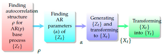
Figure 1.
A Diagram for Sample Generation Method.
2.1. Historical Seasonal Data
The obtained historical time-series data include hourly potential wind power, solar irradiance, and electric load in Texas for a year from November 2009 to October 2010 [15]. In order to obtain sample paths that indicate different seasonal characteristics, data are classified into four seasons, and the sample paths are generated for each season. Marginal distributions and autocorrelation structures for those seasonal data are found from the divided datasets separately. For solar DNI, only daytime data are used, and sample paths for nighttime are assumed to be zero without generating samples. The daytime hours for solar DNI are assumed to be from 07:00 to 19:00 h for spring and fall, 07:00 to 20:00 h for summer, and 08:00 to 19:00 h for winter, respectively.
2.2. Autocorrelation Structure of
A marginal distribution and autocorrelations of each process for solar DNI, wind power availability, and electric load are derived with the classified data, which are described in Section 2.1. Johnson’s translated systems are fit to the historical data for the marginal distributions of the process [16], whereas the Johnson’s translation system has a great flexibility for numerical analysis. Parameter estimation for the distributions is done with statistical package R. The autocorrelation structure composed of the autocorrelations of the process is represented by , where refers to the correlation between two time series, .
The autocorrelation structure of an underlying standard normal process , can be represented by , vector, and the autocorrelation, , can be found with
where
In the above Equations (1) and (2), , , and represent expectation, the standard normal cumulative distribution function, and a standardized bivariate normal distribution function, respectively. Since , , and are known in (1), the left-hand-side (LHS) value, , in (2) is known. By adjusting an unknown value, , that is implicitly incorporated in , the right-hand-side value (RHS) can be found when both LHS and RHS values are equal within a tolerance value (in this simulation, the tolerance is ). Using this method, the autocorrelation structure can be determined. The autocorrelations of the desired process and the derived stationary base process for solar DNI, wind power availability, and electricity demand with different lags, and , are listed in Table 1 and Table 2.

Table 1.
Autocorrelations of Desired Process, , With Lag p.
Table 2.
Autocorrelations of Stationary Base Process, , With Lag p.
2.3. AR(p) Parameters of Base Process
A matrix composed of variances and covariances for a standardized normal stationary process with lag p can be denoted by
’s parameters, can be found via
A random variable, , can be generated using variance which is denoted by
2.4. Generating Scenarios Using ARTA Process
In Section 2.3, the AR parameters, , and the variance , are determined. By using the parameters, a stationary AR(p) base process, , can be found as follows
where is a random variable satisfying . Once is formed, a stationary processes, , can be generated by , and the final, target process is generated. The procedure to generate random sample paths is described below:
- (1)
- Generate initial values, , using cumulative distribution functions for the historical initial value data, where p represents a lag. Initial values for , composed of the series of the differences, , are calculated, e.g., if the lag p is equal to 2, three initial values, , and , are generated, and the differences, and are obtained, where , and ;
- (2)
- Initial values for the AR(p) base process, , are generated via using the differences, s, which are derived in the previous step;
- (3)
- Generate using the AR parameters, s, where ;
- (4)
- Transform the time series, , into using ;
- (5)
- If is out of the expected, realistic range at any t, go back to Step (1), otherwise go to the next step;
- (6)
- Transform back into the target sample path with , where the initial value, , is pre-determined in Step (1).
In order to generate N random sample paths for a year, the steps described need be done for each season and are repeated N times. With the given procedure, N sample paths with AR order p = 2 for T = 24 are generated in this simulation. The generated 20 sample paths are illustrated in Figure 2. The solar DNI sample paths are generated only for daytime, as described in Section 2.1, and the values for nighttime are assumed to be zero.
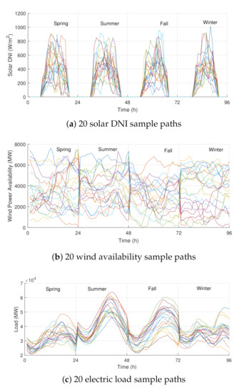
Figure 2.
Generated hourly sample paths with ARTA process for four seasons.
3. Optimization Problem
In this section, a mathematical optimization model seeking an optimal capacity of generators minimizing the building and operating costs is provided. When the optimization problem considering uncertainties is formulated, other methodologies, such as robust optimization, that are shown in the literature [17] can be applied. In this paper, a two-stage stochastic programming is selected, and the uncertainties of solar DNI, wind power availability, and uncontrollable load are consequently represented by probability distributions.
3.1. Decision Process
Within a two-stage stochastic framework [18,19], scenarios for solar DNI, wind-power availability, and electric load are represented by a scenario fan, where a sample path for 96 h representing a year (24 h for spring, summer, fall, and winter, each) is generated in the second stage as a scenario, which is shown in Figure 3.
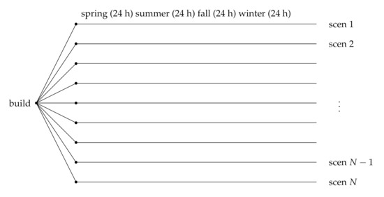
Figure 3.
A scenario fan for 96 h representing a year.
Decisions for building generators are made at the first stage. The realizations of uncertain parameters are made at the second stage, and the operation decisions including dispatching generators and procuring reserve capacity are made subsequently, with respect to the realizations of uncertain parameters.
3.2. Mathematical Model
A mathematical optimization problem seeking minimum costs is formulated with two-state stochastic programming [18,19]. The two-stage stochastic formulation is transformed into a deterministic equivalent problem with approximation of the second stage problem, and the formulation in the deterministic form is denoted by
subject to
The objective function in (7) includes approximated cost terms for generation, reserve procurement, CO emissions, and penalty costs of unserved electricity demands with respect to scenarios, where the penalty costs for unserved electricity demands and un-procured reserve are USD 30,000/MWh and USD 1000/MW, respectively, in this formulation. A carbon tax rate is assumed to be USD 10 per metric ton of CO as a fixed amount for the whole simulation.
Building decision variables for generators () are represented by binary variables in (8). The binary number indicates a decision for building or not building generators with 1 and 0, respectively. At any electric buses, the power balance implying that the injection and withdrawal of power at the bus are always the same is maintained by the constraint (9), where the continuous decision variable () represents load shedding (unserved electric demand), and it also prevents violation of the constraint. In the power balance constraint, a part of the electric load can be represented by controllable load, and electric vehicles can be modeled as a part of load as well (e.g., [20]). In this formulation, only load shedding is reflected, and the demand-side load control is not considered. Reserve capacity () is assumed to be 15% of generating power, and it is procured only from dispatchable, conventional generators in the constraint (10). The reserve procurement costs are assumed to be 10% of the generation costs by conventional generators. This type of margin is different from the operating reserve which covers short-term system changes, rather planning a reserve margin that ensures a reliable amount of generation capacity in the long-run. The deliverability of the reserve is not considered in this formulation, and only the required capacity is procured.
Constraints (11) and (12) restrict the conventional generators’ capacity for existing and newly added ones, respectively. With (12), the values representing the capacity of candidate generators () are set to zero when the generators are not built; otherwise, the capacity values are activated as pre-fixed, non-zero values. Wind-power capacity ( and for existing and candidate ones, respectively) is determined by realized wind power availability (), where are random sample paths generated by the method introduced in Section 2 for existing wind farms and for newly built farms in (13) and (14), respectively. As the uncertainty of solar DNI is realized and sample paths are generated, available solar power is estimated as in Section 4.1. For existing and candidate solar PV farms, solar power generation ( for existing and for candidate farms) is restricted by constraints (15) and (16).
In (17), active power transmitted via transmission lines () is restricted by the product of differences of voltage angles () across the line and 1/reactance, where the differences between the voltage angles are represented by bus voltage angles and the branch-node incident matrix, , which indicates the status of the linkage between electric nodes (buses) and transmission lines.
Constraint (18) also avoids overloads on transmission lines by restricting power flows in accordance with the physical thermal limits of transmission lines. The voltage angle difference between two buses connected by a transmission line is maintained within and by (19), and a voltage angle at each bus is restricted by the range, and , in (20). All decision variables for generation () need to be non-negative in (21). The mathematical formulation in Section 3 is provided in Nomenclature.
4. Simulation Results
4.1. Case Study: IEEE 300-Bus System
In order to verify if the mathematical model performs as planned, a case study with a modified IEEE 300-bus system (see [21,22]) including 411 transmission lines is performed, where the grid system is a high-voltage transmission system including several low-voltage load buses. Conventional generators (excluding solar and wind generators) in the system are coal, nuclear, conventional combustion turbine (Conv. CT), advanced combustion turbine (Adv. CT), and combined cycle gas turbine (CCGT) generators. The building and operating costs by generation technology are listed in Table 3 [23,24], where the building costs represent the annualized costs that are assumed to be 15% of overnight building costs. The number of units for solar and wind generators implicitly indicates the number of farms. Peak and average system-wide electric load are assumed to be 45% load of ERCOT (Electric Reliability Council of Texas) in 2010 [25]. Although the effects of electric vehicles and controllable load were not considered in the network, they can be modeled and applied as needed.
Table 3.
IEEE 300-bus Test System Description.
For carbon tax, CO emissions need to be calculated; therefore, emissions rates for different generator types are estimated based on [24]. Those emissions rates per MWh are listed in Table 4.
Table 4.
Cost and Emission Rates of CO [24].
The available capacity of solar PV systems using the realizations of solar DNI () is calculated by [3,26]
The area for solar PV farm installation, A, is assumed as m for 150 MW, which is the unit capacity of the solar farm. The efficiency () can be estimated based on the reference [26] as follows
where the ambient temperature, , is estimated by averaging the historical temperature data for the corresponding season and time for McCamey area in Texas [27]. The efficiency values for PV modules () and for DC/AC conversion () are assumed as 15% and 85%, respectively.
4.2. Scenario Generation Using Gaussian Copula
For a comparison purpose, scenarios representing a year are generated using Gaussian copula (GC) [28], which is a method to generate random samples using correlations and marginal distributions of random variables. Samples for each season, and day- and nighttime, are generated, and those samples form a scenario representing eight time slices, spring-daytime (sp-da in Figure 4), spring-nighttime, summer-daytime, up to winter-nighttime.
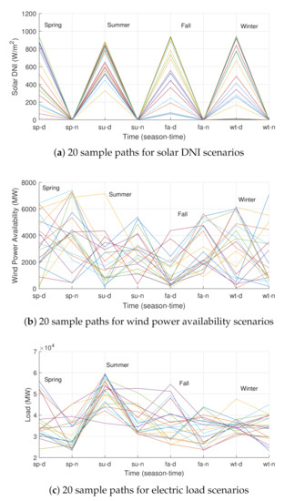
Figure 4.
Random scenarios for four seasons, day and night times with gaussian copula.
The 20 random samples by GC are illustrated in Figure 4. GC samples only indicate day- and nighttime variability and uncertainty for each season, while ARTA sample paths represent the hourly variability and chronology of stochastic parameters as well as uncertainty in the model. The differences between the scenarios by two methodologies can be compared by the two plots.
4.3. Optimal Building Capacity and Costs
The presented mathematical formulation was coded in Generic Algebraic Modeling System (GAMS) and applied to a modified IEEE 300-bus system. The CPLEX was used as an optimization solver for a mixed integer linear program [29]. In Table 5, the obtained optimal building decisions are listed to compare two cases with consideration of the seasonal, day and nighttime variability and the seasonal hourly variability. These two cases employed different scenarios generated from GC and ARTA, respectively, where scenarios from GC and ARTA are illustrated in Figure 2 and Figure 4.
Table 5.
Optimal Building Capacity & Costs Comparison.
A carbon tax with a rate of $10/metric ton was implemented as an environmental policy, and the amount of renewable generation was not mandated by policy such as renewable portfolio standards; therefore, in this simulation, wind generators and solar PV systems were built in accordance with their economic values and carbon dioxide emissions rates.
Under the carbon tax, CCGT generators, and wind and solar farms tend to be built more than other conventional generators in terms of capacity. For those generation technologies, CO emissions rates are relatively low so that the small cost increment due to carbon tax can be expected when generating electric power. Consequently, those generators are preferred to be built and operated. Coal generators are not built at all with the same rationale.
With 20 GC samples, building capacity for conventional CT and advanced CT is decreased by 337 MW compared to the 10 GC sample case, while wind-power capacity is increased by 200 MW. In terms of costs, the building cost increment was about 15.7 million dollars per year for more investment in wind capacity and less investment in CTs to 10 GC sample case, which implies that the investments in the generating units by wind resources are more attractive due to lower carbon taxes and fewer operating costs under the current simulation setup.
In the case with the 30 samples by GC, the built capacity for solar farms is the same as capacity in the case with 10 GC samples, while with the 30 sample paths by ARTA, the built capacity of solar PV systems decreases by 150 MW compared to the result with 10 sample paths.
4.4. Impacts of Hourly Variability
From the results in Table 5, the impacts on optimal decisions with and without hourly variability in the stochastic generation planning model can be compared. A noticeable change in the built capacity is observed for solar PV systems with the ARTA sample paths. The built capacity of solar PV systems with ARTA sample paths indicates a smaller value than the case using GC samples that do not consider hourly variability. The simulation model with representation of the hourly variability captures the short-term changes in solar DNI during daytime, which may diminish the economic value of solar PV systems.
Solar PV systems tend to be less economical in cases where the short-term variability is incorporated in the given stochastic generation planning model.
4.5. Computation Time
The average computation times are compared in Table 6, which reports the elapsed times in GAMS with different numbers of samples/paths. A computing machine equipped with Intel Xeon W-2135 CPU and 120 GB RAM is used for solving the presented optimization problem. We can see from Table 6 that the incremental increase in computation time is much higher with the random sample paths by the ARTA process, as the number of scenarios increases. By comparing ARTA 10, 20, and 30 scenario cases, the computation time becomes 7.67 times larger than the 10 ARTA sample path case when the number of samples is doubled from 10 to 20. In the case with 30 ARTA scenarios, the computation time becomes 21.24 times larger then 10 ARTA scenario case.
Table 6.
Elapsed Time in GAMS.
Simulations with the ARTA sample paths require much more computational time compared to the model using GC samples.
5. Conclusions
In this paper, a stochastic generation capacity planning model with hourly random sample paths reflecting the uncertainty and hourly variability of renewable resources and electric load is developed, and a case study with the IEEE 300-bus system is conducted. The obtained optimal solutions by the presented model are compared to the solutions from the stochastic model considering uncertainty and seasonal variability.
From the results, it can be concluded that accommodating the hourly variability (short-term variability) in a stochastic generation capacity planning model may lower the economic value of solar PV systems and may lead to decrease in solar PV system installation under the given condition. In other words, long-term planning models without consideration of hourly variability may overestimate the optimal capacity of solar PV systems.
6. Discussions
Long-term planning models using stochastic programming generally do not consider the short-term variability and chronology of renewable resources due to high computational efforts. Therefore, the effect of incorporating the short-term variability as well as the uncertainty has not been properly addressed, and expected changes in the economic value of renewable resources due to the short-term variability have not been examined.
One thing to be noted is that for accommodating utility-scale solar PV systems that evidently experience unavailability during nighttime and rapid changes in generation for sunrise and sunset times, the inclusion of chronology and high temporal resolution of the planning horizon have impacts on optimal generation capacity solutions in the long-term planning models. There is a tradeoff between the level of operational details in the model and computational burden in stochastic generation planning models. In many cases, very detailed operational information introduced in the model may lead to intractability of the problem. It is still challenging to obtain optimal solutions to the stochastic generation capacity planning expansion problem considering the short-term variability, and few studies introduce stochastic models incorporating the short-term variability of renewable resources due to excessive computational costs.
A limitation of the model is indeed a high computational cost. Solution times with different numbers of samples are compared in this paper, and from the comparison result we can see that incorporating the short-term variability with high resolution of the operational model dramatically increases the computational time; therefore, an optimal level of operational details needs to be found to efficiently estimate the value of uncertain, intermittent renewable resources. The high computational costs and accuracy of the operational model are tradeoffs in stochastic capacity planning models.
Funding
This work was supported by the National Research Foundation of Korea (NRF) grant funded by the Korea government (MSIP; Ministry of Science, ICT & Future Planning) (No. NRF-2017R1C1B5017348 and No. 2020R1F1A1064957).
Acknowledgments
The author also would like to thank Ross Baldick of the University of Texas and David P. Morton of Northwestern University for comments on this paper.
Conflicts of Interest
The author declares no conflict of interest.
Nomenclature
| Scenarios, sample paths | |
| Electric demand (electric load) | |
| Electric buses | |
| Transmission lines | |
| Time interval (1 h) | |
| All existing and candidate generators | |
| Existing conventional generators, | |
| Existing fossil-fueled generators, | |
| Existing wind generators, | |
| Existing solar PV generators, | |
| Candidate generators to be built | |
| Candidate conventional generators, | |
| Candidate fossil-fueled generators, | |
| Candidate wind generators, | |
| Candidate solar PV generators, | |
| , | CO emissions rate of generator r and q (metric ton/MWh) |
| , | Cost for procuring reserve from generator c and j ($/MWh) |
| Operating cost for generator g ($/MWh) | |
| Fixed reserve requirements ( %) | |
| Demand-node incidence matrix | |
| Generator-node incidence matrix | |
| Branch-node incidence matrix | |
| Annualized building cost for candidate generator n ($) | |
| , | Penalty costs on unserved demand and un-procured reserve ($/MWh) |
| Carbon tax rate on emitted CO ($/metric ton) | |
| Operating hour weight for time interval t (hour) | |
| Probability of realized sample path | |
| Capacity of conventional generator c and j (MW) | |
| Reactance of line l (p.u.) | |
| , , | Realized demand, available wind power, and solar PV generation at time t of path (MW) |
| Electric demand d of (MW) | |
| , | Availability of solar PV generator s and candidate solar PV m of (MW) |
| , | Availability of wind generator w and candidate wind generator k of (MW) |
| , , | Decision to build candidate generator n, j, k |
| , , , , | Generation of generator g, c, r, w, and s (MW) |
| , | Reserve procured from generator c and j (MW) |
| , , , , | Generation of candidate generator n, j, q, k, and m (MW) |
| Power flow on transmission line l (MW) | |
| Unserved electric demand (MW) | |
| Voltage angle at bus i (radian) | |
| Un-procured reserve (MW) | |
References
- Gil, E.; Aravena, I.; Cárdenas, R. Generation capacity expansion planning under hydro uncertainty using stochastic mixed integer programming and scenario reduction. IEEE Trans. Power Syst. 2015, 30, 1838–1847. [Google Scholar] [CrossRef]
- Dehghan, S.; Amjady, N.; Conejo, A.J. Reliability-Constrained Robust Power System Expansion Planning. IEEE Trans. Power Syst. 2015, 31, 2383–2392. [Google Scholar] [CrossRef]
- Park, H.; Baldick, R. Optimal capacity planning of generation system integrating uncertain solar and wind energy with seasonal variability. Electr. Power Syst. Res. 2020, 180. [Google Scholar] [CrossRef]
- Sadeghia, H.; Rashidinejada, M.; Abdollahia, A. A comprehensive sequential review study through the generation expansion planning. Renew. Sust. Energy Rev. 2017, 67, 1369–1394. [Google Scholar] [CrossRef]
- Shortt, A.; Kiviluoma, J.; Malley, M.O. Accommodating Variability in Generation Planning. IEEE Trans. Power Syst. 2013, 28, 158–169. [Google Scholar] [CrossRef]
- Haydt, G.; Leal, V.; Pina, A.; Silva, C.A. The relevance of the energy resource dynamics in the mid/long-term energy planning models. Renew. Energy 2011, 36, 3068–3074. [Google Scholar] [CrossRef]
- Ludig, S.; Haller, M.; Schmid, E.; Bauer, N. Fluctuating renewables in a long-term climate change mitigation strategy. Energy 2011, 36, 6674–6685. [Google Scholar] [CrossRef]
- Jin, S.; Botterud, A.; Ryan, S.M. Temporal Versus Stochastic Granularity in Thermal Generation Capacity Planning With Wind Power. IEEE Trans. Power Syst. 2014, 29, 2033–2041. [Google Scholar] [CrossRef]
- Pereira, S.; Ferreira, P.; Vaz, A.I.F. Generation expansion planning with high share of renewables of variable output. Appl. Energy 2017, 190, 1275–1288. [Google Scholar] [CrossRef]
- Pina, A.; Silva, C.A.; Ferrão, P. High-resolution modeling framework for planning electricity systems with high penetration of renewables. Appl. Energy 2013, 112, 215–223. [Google Scholar] [CrossRef]
- Merrick, J.H. On representation of temporal variability in electricity capacity planning models. Energy Econ. 2016, 59, 261–274. [Google Scholar] [CrossRef]
- Seljoma, P.; Tomasgard, A. Short-term uncertainty in long-term energy system models—A case study of wind power in Denmark. Energy Econ. 2015, 49, 157–167. [Google Scholar] [CrossRef]
- Cario, M.C.; Nelson, B.L. Autoregressive to anything: Time-series input processes for simulation. Oper. Res. Lett. 1996, 19, 51–58. [Google Scholar] [CrossRef]
- Cario, M.C.; Nelson, B.L. Numerical Methods for Fitting and Simulating Autoregressive-to-Anything Processes. INFORMS J. Comput. 1998, 10, 72–81. [Google Scholar] [CrossRef]
- SolarAnywhere. Available online: https://www.solaranywhere.com/ (accessed on 25 October 2020).
- Johnson, N.L. Systems of frequency curves generated by methods of translation. Biometrika 1949, 36, 149–176. [Google Scholar] [CrossRef] [PubMed]
- Malcolm, S.A.; Zenios, S.A. Robust Optimization for Power Systems Capacity Expansion under Uncertainty. J. Oper. Res. Soc. 1994, 45, 1040–1049. [Google Scholar] [CrossRef]
- Birge, J.R.; Louveaux, F. Introduction to Stochastic Programming; Springer: New York, NY, USA, 1997. [Google Scholar]
- Shapiro, A.; Dentcheva, D.; Ruszczynski, A. Lectures on Stochastic Programming; MPS-SIAM: Philadelphia, PA, USA, 2009. [Google Scholar]
- Shen, J.; Jiang, C.; Li, B. Controllable Load Management Approaches in Smart Grids. Energies 2015, 8, 11187–11202. [Google Scholar] [CrossRef]
- University of Washington. Power Systems Test Case Archive. Available online: https://www2.ee.washington.edu/research/pstca/pf300/pg_tca300bus.htm (accessed on 25 October 2020).
- Illinois Center for a Smarter Electric Grid. IEEE 300-Bus System. Available online: http://icseg.iti.illinois.edu/ieee-300-bus-system/ (accessed on 25 October 2020).
- U.S Energy Information Administration. Annual Energy Outlook. 2017. Available online: https://www.eia.gov/outlooks/archive/aeo17/ (accessed on 25 October 2020).
- U.S Energy Information Administration. Updated Capital Cost Estimates for Utility Scale Electricity Generating Plants. 2016. Available online: https://www.eia.gov/analysis/studies/powerplants/capitalcost/ (accessed on 25 October 2020).
- The Electric Reliability Council of Texas Website. Available online: http://www.ercot.com/gridinfo/load/forecast/ (accessed on 25 October 2020).
- Duffie, J.A.; Beckman, W.A. Solar Engineering of Thermal Processes; Wiley: New York, NY, USA, 2013. [Google Scholar]
- U.S Climate Data. Available online: www.usclimatedata.com/climate/mccamey/texas/united-states/ustx0855/2010/1 (accessed on 25 October 2020).
- Cario, M.C.; Nelson, B.L. Modeling and Generating Random Vectors with Arbitrary Marginal Distributions and Correlation Matrix. 1997. Available online: http://citeseerx.ist.psu.edu/viewdoc/download?doi=10.1.1.48.281&rep=rep1&type=pdf (accessed on 25 October 2020).
- GAMS Documentation 25.1. Available online: https://www.gams.com/latest/docs/S_CPLEX.html (accessed on 25 October 2020).


Publisher’s Note: MDPI stays neutral with regard to jurisdictional claims in published maps and institutional affiliations. |
© 2020 by the author. Licensee MDPI, Basel, Switzerland. This article is an open access article distributed under the terms and conditions of the Creative Commons Attribution (CC BY) license (http://creativecommons.org/licenses/by/4.0/).