1. Introduction
In the transient analysis [
1,
2] of a distribute circuit model of a busbar [
3,
4,
5,
6,
7], the order of equation sets is extremely high. Meanwhile, model order reduction (MOR) techniques [
8], such as the proper orthogonal decomposition (POD)-based MOR approach [
9,
10,
11,
12], the data-driven MOR method [
13], the nonlinear MOR technique [
14], and the dynamic mode decomposition (DMD)-based MOR approach [
15], have all been proven to be very effective in combating such a high complexity issue. Compared with these reduction methods, the structure-preserving reduced-order interconnect macromodeling (SPRIM) based on Krylov subspaces, built on the Arnoldi algorithm [
16], can achieve a higher order reduction radio and accuracy for large multi-port Resistor-Capacitor-Inductor (RCL) circuits [
17,
18,
19,
20,
21]. The Krylov subspace based MOR method is aimed at matching the moments [
22] at a special point,
s0, so that the reduced-order system can effectively replicate the dynamic response of the original system’s transfer function around the expansion point
s0. Obviously, this type of MOR methods will replicate the dynamic response of the original system in a small band of the selected frequency
s0 with a very high accuracy [
8]. Consequently, the Krylov subspace-based MOR method is widely used as a standard model order reduction technique by engineers and academicians. However, for a very wide frequency transients, the performance of a Krylov subspace based MOR method is not satisfactory. Moreover, the selection of the expansion point
s0 has not been comprehensively studied in the literature. As a result, one needs to readjust the expansion point
s0 according to a rule of thumb until the accuracy of the results satisfies the predefined tolerance requirement.
As is well known, with the continuous advancement in power electronics technology and the rapid implementation of power electronic devices, the switching frequency of a power electronic value, such as an insulated-gate bipolar transistor (IGBT), increases tremendously. Therefore, the turn-on and turn-off transients of an IGBT-based inverter cover a very wide band of frequencies. In this regard, the existing SPRIM cannot guarantee the precision of the reduced-order model in a broadband frequency range. To overcome these shortcomings of the existing SPRIM, a broadband enhanced SPRIM method is proposed in this paper.
2. Broadband SPRIM Methodology
For a
p-port RLC interconnect network, its circuit equations in a time-domain modified nodal analysis (MNA) [
17] are:
and the corresponding compact form is:
where
and
are the
nth nodal voltage (
n = 1, …,
N) and the
LSth branch current (
LS = 1, …,
M including voltage sources and inductances), respectively;
and
are the input voltage sources and output currents, respectively;
is an identity matrix;
,
, and
are the submatrices of the capacitances, the inductances, and the resistances, respectively; and
consists of 1 s, −1 s, and 0 s, representing the current variables in the Kirchhoff Circuit Law (KCL) equations.
As explained previously, the SPRIM algorithm is a Krylov subspace-based moment matching MOR technique. The moments are defined as the Taylor series coefficients of the system transfer function. For an expansion point
s0 (
is nonsingular), the transfer function of the proposed full-order model for a liner subsystem is expanded into the Taylor series at
s0 as:
where
is the
ith moment of the system at the expansion point
s0.
In the SPRIM algorithm, is defined as the dimension of the generated Krylov subspace and its value is equal to the integral multiple of the number of input-output ports (, r = 1, 2…). Using the SPRIM algorithm, the order of the MOR model will be reduced from (N+M) to 2n. Meanwhile, the full-order moment and MOR moment satisfy . Therefore, by choosing an integer r and an expansion point s0, the first 2r terms of the moments of the full-order model are exactly matched at the expansion point s0.
The expansion point s0 is usually chosen by a user according to their knowledge on the transient characteristics of the system, and one s0 can only guarantee a relatively high precision of the reduced-order model around a specified frequency range, i.e., it cannot guarantee the accuracy of the reduced-order model in a broadband frequency range. To overcome this deficiency, an adaptive broadband SPRIM is proposed in this article, and explained in details (Algorithm 1).
To start, the following terminologies and formulations are introduced and used.
First, to avoid the deficiency in deciding the expansion point
s0, i.e., to automatically find the best
s0 at each frequency, a single objective optimization problem, the minimization of the deviation of the responses between the full-order system and the reduced order system, is formulated as:
where
P is the number of the total ports, and
and
are the
pth output variables of the full-order system and the reduced order system, respectively. One then can utilize an intelligent computing method such as the simulated annealing algorithm [
23] and genetic algorithms [
24] to solve the single objective optimization problem. In this paper, the well-known genetic algorithm [
24] is used.
Second, by applying fast fourier transform (FFT) to the exciting signal of the system, one obtains its time domain expression as:
where, the magnitudes
mis satisfy
, i.e., each item is sorted according to its magnitude. For each frequency component
, one defines:
where, ”[x]” means to take the largest integer which is smaller than the real number x, and subsequently constructs array {
}.
It should be noted that there will be cases where two or more his elements are equal in array {}, i.e., . Consequently, one will retain his with different magnitudes, forming a new array {} ().
To facilitate the explanation, one defines “individual” as the basis of a specific frequency by directly solving (4); “element” as the projected basis of the “individual” using an orthogonal normalization operation; and the excitation signal as the “test set”, i.e., use the reduced-order model to calculate the response of “test set” to measure the current transformation matrices of a MOR.
Using these terminologies and formulations, the details of the proposed broadband enhanced SPRIM method are explained as follows.
Initially, evaluate the frequency band (fmin ~ fmax, “~”means “to”) of the dynamic performances according to the energy distribution of the excitation signal. Finding the optimal expansion points smin and smax at the minimum frequency fmin and the maximum frequency fmax, respectively, from (4); evaluate the projection basis Vmin and Vmax for fmin and fmax, respectively; perform an orthogonal normalization operation on Vmin and Vmax to obtain a new transformation matrix V0; and the proposed broadband SPRIM methodology will then move to the following MOR procedures. Since V0 is the 1st “element”, choose frequency h1 (), i.e., choose the first element in {} (the largest magnitude one in hi) and perform an orthogonal normalization operation on this “individual” and V0 to produce the 2nd “element” V1; calculate, respectively, the responses of the reduced-order models constructed by V0 and V1 using the “test set”; if the relative error satisfies the predefined tolerance criterion, stop the iterative procedure and output the transformation matrices and the coefficient matrices of the reduced system; otherwise, chose another frequency h2 () (the second largest element in {}) and calculate the corresponding “individual”, perform an orthogonal normalization operation on this “individual”, and V1 to yield a new V2; calculate, respectively, the responses of the reduced-order models constructed by V1 and V2 using the “test set”, and evaluate their relative error, if the relative error satisfies the predefined tolerance criterion, stop the iterative procedure and output the reduced order model results; otherwise start a new cycle of frequency sampling and repeat the above iterative procedure until the solution satisfies the error control rule. The following paragraphs give a detailed explanations of the iterative procedures of the proposed methodology.
| Algorithm 1: The proposed broadband enhanced SPRIM methodology |
| Input: | The coefficient matrices of the full-order system (C, G, B) and the range of the broadband frequency and the tolerance of the relative error . |
| | Step 1: Calculate the optimal expansion point and construct the projection basis. |
| | (1.1): Use genetic algorithm to solve Equation (4) to obtain the optimal expansion point: |
| | , |
| | (1.2): Construct the projection basis by the block Arnoldi algorithm [16]: , |
| | (1.3): Perform an orthogonal normalization operation as |
| | Step 2: |
| | Step 3: |
| | Step4: |
| | (4.1): [21], |
| | (4.2): |
| | (a) |
| | (b) |
| | (4.3): |
| | (4.4) Compute the former reduced matrices |
| | (4.5) |
| | (4.6) Compute the current reduced matrices |
| | (4.7) , compute the solutions |
| | (a) Obtain the solution y0 by solving the Equation (1) under |
| | (b) Obtain the solution y1 by solving the Equation (1) under |
| | (4.8) |
| | (4.9) |
| | Step5: End |
| Output: The coefficient matrices of reduced system . |
Once the projection matrix
Q is obtained, it will be used to yield a reduced model of:
where
,
,
.
3. Numerical Application and Discussion
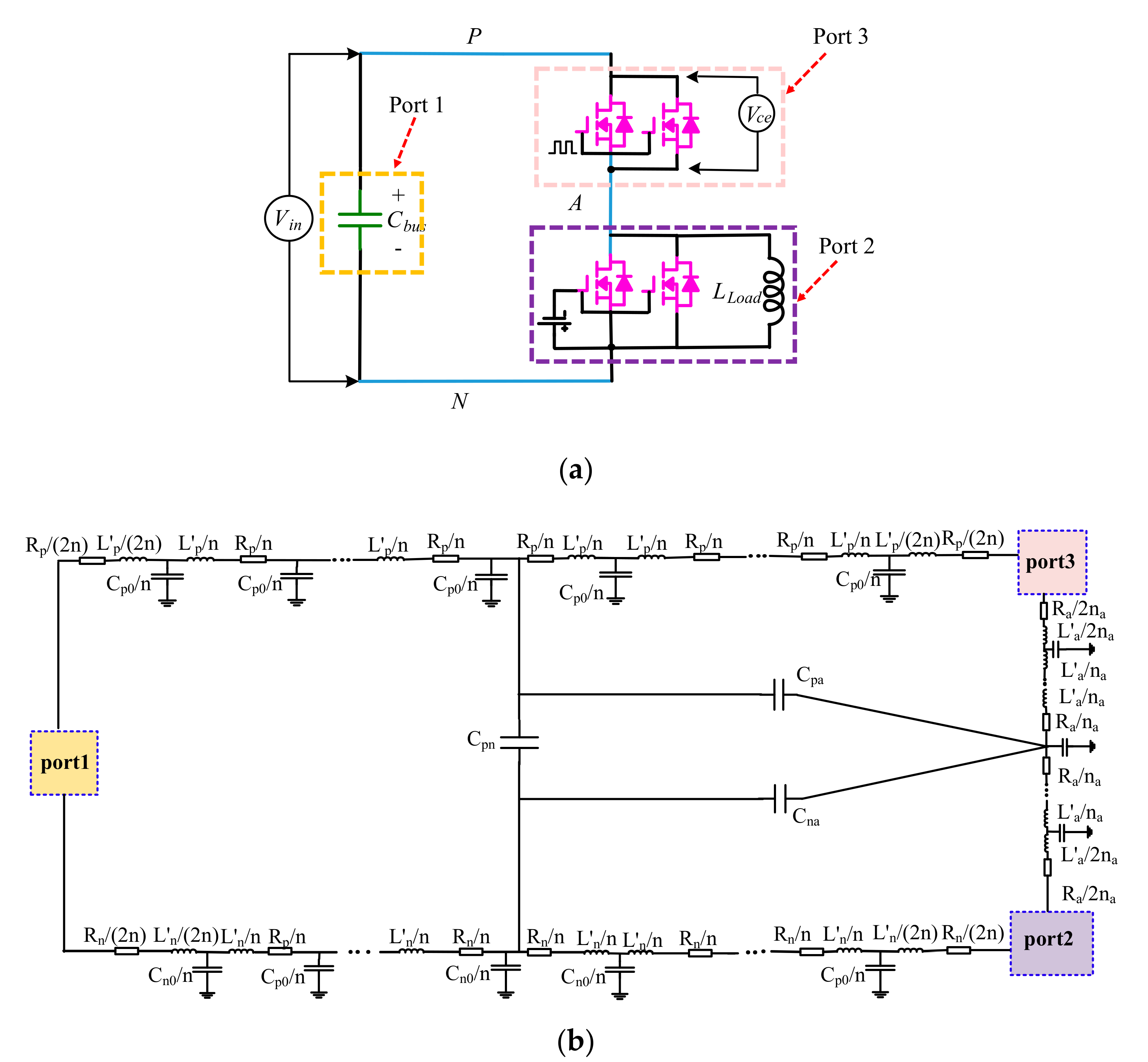
The proposed broadband enhanced SPRIM method is used for the order reduction of the multi-port RLC circuits of a prototype IGBT-based inverter busbar. The IGBT is a FZ2400R17KE3 (1700 V/2400 A). The single-phase double pulse test circuit (
Figure 1a) of the IGBT based inverter is modeled by a multi-sectional equivalent circuit model, as given in
Figure 1b. The whole busbar (
Figure 1) includes a positive busbar (the segment between port 1 and port 3), a negative busbar (the segment between port 1 and port 2), and a phase output copper bar (the segment between port 2 and port 3). For each sectional model, a T type circuit is used, and the circuit parameters, inductance, the resistance, self-capacitance and mutual capacitance between any two conductors are calculated from the harmonic electromagnetic field solution. The division and number of the multi-sections of the whole circuit model are decided according to the busbar geometry and length.
To validate the proposed model and methodology, it is used to predict the transient current response of a prototype IGBT-based inverter excited by a square wave (
f = 10
7 Hz, duty cycle = 0.1, and duty cycle = 0.5, respectively) and a tested turn-off voltage signal excitation.
Figure 1b shows the full-order equivalent circuit of the current communication loop. In the model, the yellow, pink, and purple area represent the DC bus stabilized capacitor, IGBT to be tested, and counterpart IGBT, and are considered as port 1, port 3, and port 2, respectively. The rest of the equivalent circuit models without any color enclose line are the macromodeling of the interconnect busbar for the fast turn-on and turn-off transients. Consequently, the equations related to the circuit models without any color enclose line will be order reduced. To compare the proposed broadband SPRIM (bbd-SPRIM) model with the SPRIM model, the transient response of port 1–3 (y
1–y
3) is computed using SPRIM and the proposed methodology, respectively.
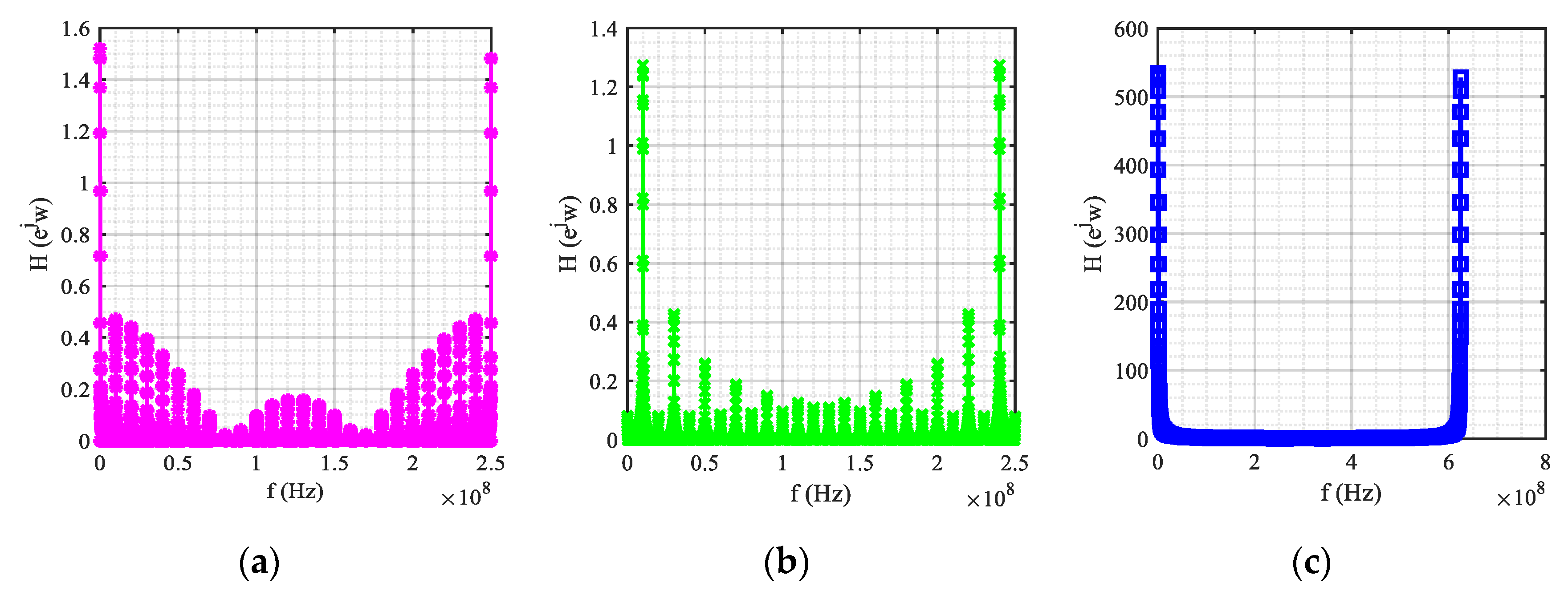
According to the spectrum analysis of the excitation signal (
Figure 2), choose
,
,
. The finally used frequency samples are
,
, and
Hz. The full seize of the equivalent circuit is 78, and its reduced seize using the proposed methodology is 18. However, as the seize of the reduced model is an integer multiple of the number of the ports, we compare the two reduced models with 12 and 18 sizes, respectively. Moreover, for performance comparisons, one uses the following two metrics to measure the relative errors between the responses of the reduced model and full-order model. The first one is expressed as:
where
(= 1, 2, 3) represents the
ith input-output port, and
and
represent the output responses of the
ith port from the reduced model and the full-order model, respectively.
The second one is used to illustrate the transient characteristics of the relative errors with respect to time, and is defined as:
where
and
represent the responses of the reduced model and full-order model on the
jth sampling point.
For the SPRIM algorithm, the reduced-order system can effectively imitate the dynamic response of the original system around the expansion point
s0. If
s0 = 0, the reduced-order system is able to reproduce the dynamic response of the original system in the low-frequency range. If
s0 = ∞, the reduced-order system is able to approximate the dynamic response of the original system in the high-frequency range. Since the response in our case (
Figure 2) is a wideband frequency one and is mostly in a high frequency band, one selects
and
, respectively for the SPRIM algorithm. Therefore, for comparing the proposed bbd-SPRIM model with the SPRIM model comprehensively, one compares the proposed SPRIM model with the SPRIM model under two different expand points, i.e.,
and
. It should be noted that all comparisons between the proposed SPRIM model and SPRIM model are under the same model size.
The transient relative errors of the proposed bbd-SPRIM model and original SPRIM under different model sizes are given in
Figure 3,
Figure 4 and
Figure 5, respectively, while the relative errors of the proposed bbd-SPRIM model and original SPRIM under different model sizes are tabulated in
Table 1 and
Table 2, respectively.
The relative errors in the tables is arranged in (a, b, c): The first one (a) corresponds to the result from SPRIM using
, the second one (b) corresponds to the result from SPRIM using
, and the third one (c) corresponds to the result from the proposed bbd-SPRIM. From the numerical results in
Table 1, it is easy to observe that for a dynamic response to these three case studies, i.e., a square wave (
f = 10
7 Hz, duty cycle = 0.1), a square wave (
f = 10
7 Hz, duty cycle = 0.5), and the tested turn-off signal, the relative errors of port 1 and port 3 of the reduced model from the SPRIM (
) are the largest ones when compared to those of the other two reduced models, while the relative errors using the proposed bbd-SPRIM are the smallest ones. Moreover, for a dynamic response to these three excitations, the transient relative errors of port 2 of the reduced model using the original SPRIM (
) is the largest ones when compared to those of the other two reduced models. Roughly observing, the relative errors of the proposed bb-SPRIM are obviously smaller than the other two reduced-order models except the relative error of port2 under a tested turn-off signal excitation. In other words, the relative error of port2 using the proposed bbd-SPRIM model is higher than that of the SPRIM model with
but still smaller than that of the SPRIM model while
. Moreover, since the smallest relative error of the reduced model exceeds 1, it is necessary to increase the size of the reduced model under a turn-off signal excitation.
As the size of the reduced model is an integer multiple of the number of the input-output ports, and normally, the size of the reduced model is higher, the relative error of the reduced model to the original model is smaller. In this regard, one compares the relative errors in a 18 reduced order model in
Table 2. From the numerical results in
Table 2, it is easy to observe that the relative errors of the three reduced models are smaller than those of the corresponding 12 reduced order models. Meanwhile, the relative errors of the reduced model using the proposed SPRIM methodology is the smallest one when compared to the other two reduced models using SPRIM.
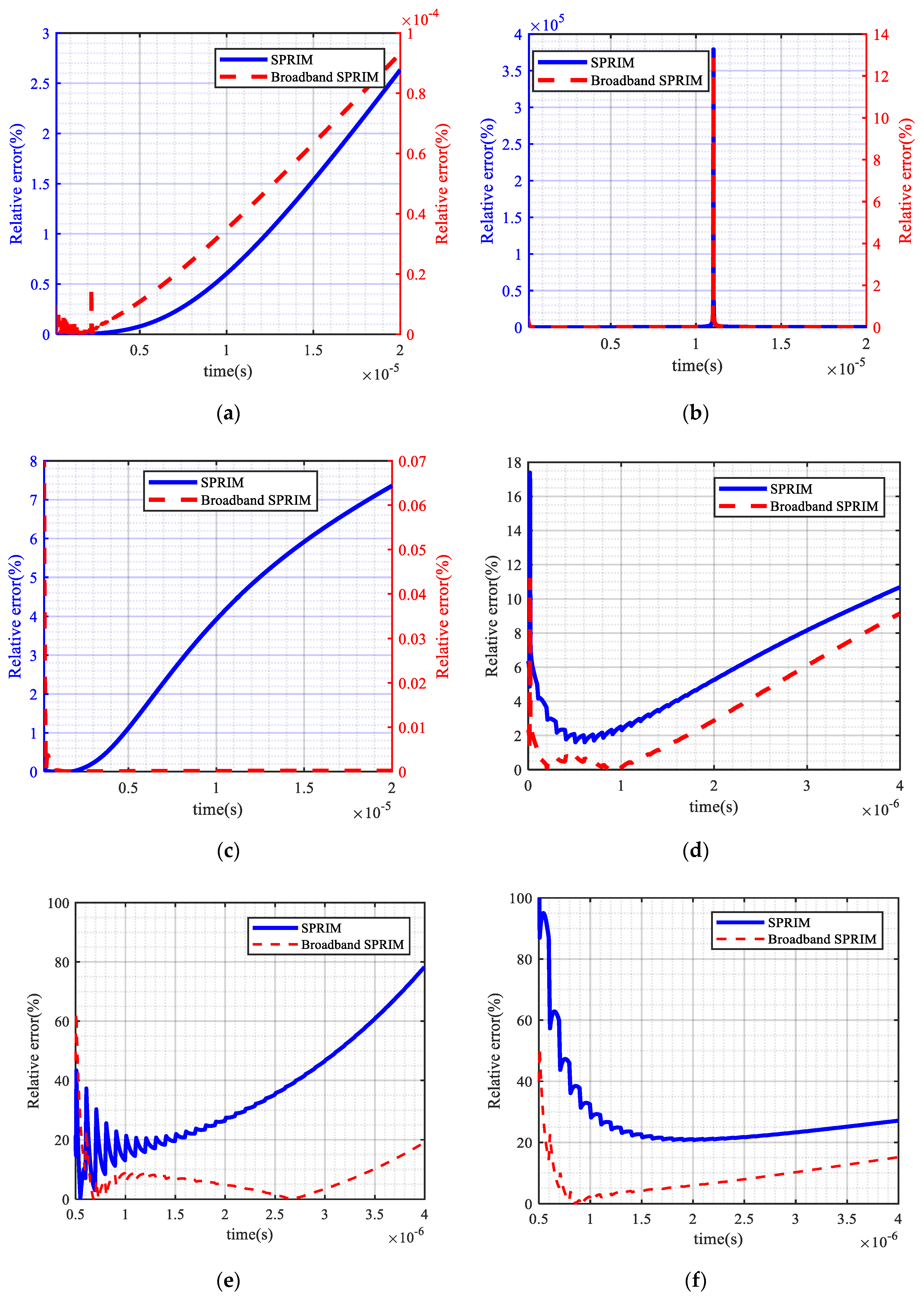
Figure 3a–c gives the transient relative errors between the computed response of the three ports using the two reduced-order models and full-order equivalent circuit model under the tested turn-off signal excitation, while (d) to (f) present the results under a square wave excitation of frequency
f = 10
7 Hz, duty cycle = 0.1. It should be noted that the expansion point
s0 is chosen randomly according to the energy distribution of the excitation signal and the traditional selection rule in this paper if without any specific description, and its values in different cases are explained in the corresponding paragraphs.
From the numerical results (
Figure 3a–c), it is easy to observe that for a dynamic response to the tested turn-off signal, the transient relative errors of the two reduced-order models have some differences: For port 1, the relative errors of the two reduced-order models will increase with time, but the relative error of the proposed bbd-SPRIM model is four orders of magnitude smaller than that of the SPRIM model; for port 2, both of the curves have a peak, but the value of the peak of the proposed bbd-SPRIM model is four orders of magnitude smaller than that of the SPRIM model; for port 3, the relative error of the proposed bbd-SPRIM model decreases with time while that of the SPRIM model increases with time. The maximum relative error of the proposed bbd-SPRIM model does not exceed 0.07%, while that of the SPRIM model reaches 7.5%. From the numerical results (
Figure 3d–f), it is easy to observe that for a dynamic response to a square wave (
f = 10
7 Hz, duty cycle = 0.1) excitation, the numerical results of the two reduced-order models have minor differences: For port 1, the relative errors of the two reduced-order models are almost identical, but the error of the SPRIM model is still higher than that of the proposed bbd-SPRIM model, as the maximum error of the SPRIM model can reach 17% but the one of the proposed model does not exceed 11%; for port 2, roughly observing, the relative error if the SPRIM model increases in the time span while that of the proposed bbd-SPRIM model decreases with time as a whole. Thus, the maximum error of the proposed model exists in the beginning of the time and excluding the beginning of the time, the error of the proposed model does not exceed 20%, while that of the SPRIM model reaches 80%; for port 3, the shape and direction of the curves of the two reduced-order models are almost identical, but the relative error of the proposed model is always smaller than that of the SPRIM model. Besides, the error of the SPRIM model is always more than 20% and the maximum error reaches 100%, while the maximum error of the proposed model does not exceed 50% and except at the beginning, the relative error of the proposed model is smaller than 20%.
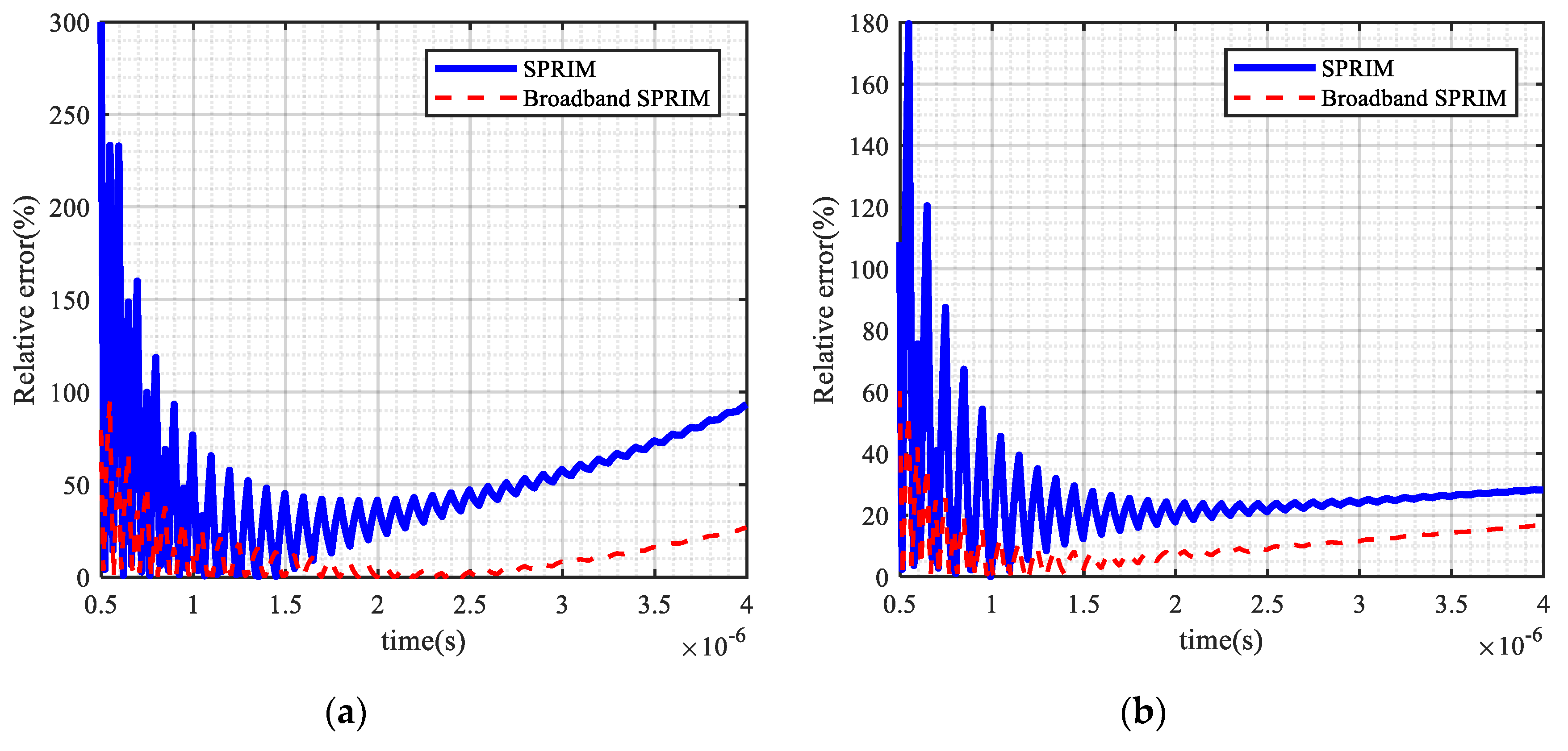
Figure 4 presents the relative errors of the reduced models of SPRIM and proposed SPRIM to those of the full-order circuit model under a square wave excitation of frequency
f = 10
7 Hz, duty cycle = 0.5. It is obvious that the numerical results of the two reduced-order models have some differences. The relative errors of the SPRIM model is always higher than that of the proposed bbd-SPRIM model: For port 2, the maximum relative error of the bbd-SPRIM model is 95.1%, while that of the SPRIM model reaches 300%; for port 3, the maximum relative error of the bbd-SPRIM model is 61%, while that of the SPRIM model reaches 180%.
Figure 5 presents the relative errors of the reduced model of SPRIM using different expansion point
s0 and the proposed broadband SPRIM to those of the full-order circuit model under a square wave excitation of frequency
f = 10
7 Hz and duty cycle = 0.1.
Figure 5a gives the comparison of the relative errors of the 12 reduced order models while
Figure 5b gives the comparison of the relative errors of the 18 reduced order models. From the numerical results in
Figure 5a, it is easy to observe that the relative error of the SPRIM model depends on the value of the expansion point
s0. Moreover, in one time span, the relative error of the reduced model of SPRIM on one expansion point is smaller than that of the other expansion point and in another time span, it will be higher. As is shown in
Figure 5a, in the time span (0–1.2 μs), the relative error of the reduced model on
is smaller than that of
, but in the time span (1.2–4 μs), the relative error of the reduced model on
is higher than that of
. However, the relative error of the proposed bb-SPRIM model is always smaller than that of the SPRIM model irrespective of the expansion point selection (
Figure 5a,b).
Moreover, for the full-order equivalent circuit model of the prototype IGBT-based inverter busbar, the computing time for a transient process of the total 2000 turn-off wave cycles is about 2940 s, while for the proposed bbd-SPRIM model it is less than 1300 s. Although the computational time required to solve the optimization problem is about 100 s and the computational time for implementing the rest of the proposed broadband SPRIM is about 25 s, the total CPU time (1425 s) of the proposed reduced-order model is still much smaller when compared to 2940 s.


