Event Effects Estimation on Electricity Demand Forecasting

Abstract

We consider the problem of short-term electricity demand forecasting in a small-scale area. Electric power usage depends heavily on irregular daily events. Event information must be incorporated into the forecasting model to obtain high forecast accuracy. The electricity fluctuation due to daily events is considered to be a basis function of time period in a regression model. We present several basis functions that extract the characteristics of the event effect. When the basis function cannot be specified, we employ the fused lasso for automatic construction of the basis function. With the fused lasso, some coefficients of neighboring time periods take exactly the same values, leading to stable basis function estimation and enhancement of interpretation. Our proposed method is applied to the electricity demand data of a research facility in Japan. The results show that our proposed model yields better forecast accuracy than a model that omits event information; our proposed method resulted in roughly 12% and 20% improvements in mean absolute percentage error and root mean squared error, respectively.

1. Introduction

After Japan fully liberalized its retail power operation in April 2016, the number of power producers and suppliers (PPSs), that is, electricity utilities other than the ten dominating general electricity utilities, has increased significantly. The PPSs’ share of electric power sales in Japan is shown in Figure 1 [1]. Their total share has significantly increased from April 2016 to June 2020 in all areas. In particular, the share approaches 25% in the Tokyo area in 2020.

Nowadays, PPSs procure more than 80% of their total supply power from the Japan Electric Power Exchange (JEPX [2]), as shown in Figure 2. Although their backup power remains low, their electric power procurement has significantly increased in the last two years, especially from September 2018 to December 2018. The reduction in procurement cost in the JEPX market has been crucial for PPSs.

In JEPX, the day-ahead (or spot) and intraday markets are popular in electricity exchanges. In the day-ahead market, contracts are made for the delivery of electricity on the following day. In the intraday market, power will be delivered one hour after the order is closed. In both markets, transactions are typically made in 30-min intervals. Therefore, suppliers must provide 48 forecast values per a day.

Participating in JEPX involves the risk of an increase in procurement cost. For example, JEPX imposes an imbalance fee based on the difference between the actual and forecasted power demand. Another risk is the fluctuation in electricity prices. In the day-ahead market, bidding is done by a single price auction system; the cost is determined by the intersection of the demand and supply curves. Therefore, electricity price is highly affected by the Japanese economy, such as oil prices. Thus, an accurate forecasting method is essential for PPSs to reduce their procurement cost [3]. A review of the existing forecasting techniques is presented in Section 2.

PPSs have to forecast their electricity demands for ten supply areas separately, as shown in Figure 1. The PPSs have a different number of customers in each area. Some areas may have a large number of customers. In large-scale areas, the forecast accuracy would be high even if one or a few customers change their electricity usage pattern due to some daily event because the event effect would be small compared to the total electricity demand [4]. Thus, the forecast is typically based on past demand and weather information, for example, temperature [5] and humidity [6]. However, many PPSs could have a small number of customers in one of their supply areas. Indeed, from the data available at the Energy Information Center in Japan [7], 218 PPSs traded less than 1000 MWh of electricity in April 2020 [7]. For small-scale areas, the electricity fluctuation due to a specific customer’s daily event can have considerable effect on the total electricity demand. A forecast without incorporating event information can lead to poor forecast accuracy. Therefore, it is crucial to incorporate event information into forecasting models for small-scale areas.

Figure 3 shows the daily demand of a research facility in 2018 (This facility is in the Kyushu region; we cannot provide further details of this research region for confidentiality reasons). The average temperature near the facility is also provided.

Some of the demand data figures are not depicted owing to missing values or outliers, resulting in 353 complete daily demands in 2018. The average temperature has considerable influence on the demand. Indeed, the demand becomes high when the temperature is either high or low owing to air conditioner usage. In Japan, air conditioners are mainly used as a heating system in the winter season (see, e.g., in [8]). We consider the relationship between temperature and demand in detail in Section 4.2. We also observe that daily demand has a weekly seasonality. However, daily demand cannot be approximated from only the effects mentioned above. Indeed, some daily demands are exceptionally large apart from weekly seasonality. An irregular event causes the instability of demand; this facility irregularly consumes a large amount of electricity due to some experiments.

To illustrate the event effects in more detail, we depict the half-hourly electricity demand of the research facility in November 2018 in Figure 4.

Electricity demand shows weekly seasonality: demand is high on weekdays and low on weekends (4, 11, 18, and 25 November are Sundays). The routine human activity may cause daily variation during weekdays. However, we observe a significant difference in demand pattern for the same day of the week. For example, the maximum demand on 28 November was much larger than that on 21 November. An irregular event caused this large electricity demand on 28 November. We aim to construct a forecasting model that incorporates the effect of such irregular daily events.

As mentioned earlier, a large number of methodologies are available for electricity demand forecasting (please refer to Section 2 for details). Most methods do not consider event information. To incorporate the event effects into a forecasting method, we typically transform the event information into a dummy variable (i.e., a variable that takes 1 when an event occurs, and 0 otherwise) and add it to the exploratory variables. This approach reduces to the standard regression analysis or machine learning techniques. Indeed, Grolinger et al. [9], Grolinger et al. [10] used a dummy variable to show improvement in forecast accuracy.

However, the dummy variables approach has limitations in that it cannot incorporate detailed information on the daily event. For example, assume that the irregular event is factory operation. The electricity usage pattern of the factory can manage load shifting (see, e.g., in [11]); therefore, we can “roughly” find the electricity fluctuation due to factory operation on each time period in advance. Such detailed event information is expressed as a function of the time period. The dummy variables approach cannot directly incorporate the time period function because the dummy variables take only either 0 or 1 for each time period. Thus, the dummy variables approach disregards useful information on the daily event. To incorporate time-varying electricity fluctuation information, we must view the event effect as a time period function.

To incorporate a wide variety of event effects that depend on the time period, we employ basis expansion [12,13]; the event effect is expressed as a basis function depending on the time period. The basis function approach generalizes the dummy variable; indeed, the indicator function corresponds to the dummy variable. Moreover, the basis function expresses the event effect much more flexibly than the dummy variable. For example, Hirose [14] recently proposed a statistical model based on the varying-coefficient model with basis expansion, employing the B-spline function as basis function to capture the COVID-19 effect. This study adopts the forecasting model used in [14] because the numerical results show that his forecasting technique outperformed several existing machine learning techniques.

The B-spline function is known as a smooth function. However, most event effects are expressed as a non-smooth function due to a sudden change in electricity usage. Examples include the illumination in a stadium, factory operations, experiments, and supercomputers. In this study, we use event-specific basis functions. For example, when an event is in some specific time period, the basis function takes 1 for that time period, and 0 otherwise. A more flexible basis function can be constructed according to the event characteristics. The details are presented in Section 3.2.1.

A basis function can be constructed only when detailed information on the event is provided. However, in many cases, we do not have enough event information to specify the basis function. Indeed, PPSs enter into many contracts, and it would be difficult to obtain all information on each customer’s events in detail. For the above-mentioned demand data in a research facility depicted in Figure 3 and Figure 4, we do not have detailed information on the events (i.e., experiments). Therefore, we find it important to extend our proposed method even when the basis function cannot be specified; in other words, we need a procedure for automatic construction of the basis function.

To automatically generate a non-smooth basis function, we employ the fused lasso [15]. With the fused lasso, we can estimate some of the parameters in the neighbouring time periods as exactly the same values, greatly enhancing the interpretation of the basis function. The fused lasso includes a regularization parameter that controls the degree of simplicity of the basis function. For example, when the regularization parameter is sufficiently large, the basis function becomes an indicator function (i.e., dummy variables), and as it becomes small, the basis function becomes complex. We select the regularization parameter so as to minimize the forecast error. The fused lasso is typically used in life science studies (e.g., gene expression data analysis) and image processing [16], but to our knowledge, application of the fused lasso to electricity demand forecasting has not yet been examined.

The remainder of the paper is organized as follows. Section 2 briefly reviews the existing forecasting techniques. Section 3 presents our proposed method based on basis expansion both with and without basis function specification. In particular, Section 3.2 describes the main idea of our proposed method. We apply our proposed method to the electricity demand data from a research facility in Section 4. The conclusions and future direction of the study are presented in Section 5.

2. Literature Review

Many forecasting methods are proposed in the literature. The forecasting techniques are classified mainly into two approaches, statistical and machine learning approaches. The former builds a statistical model based on data characteristics. Several statistical models are interpretable, making it easy to develop strategies for energy-saving intervention (see, e.g., in [17,18]) and demand response (see, e.g., in [19]). Furthermore, most of the statistical methods are based on probabilistic forecasting, and therefore, it is easy to construct the prediction interval. The review of probabilistic forecasting is presented in [20]. Another approach to investigate uncertainty is to employ the fuzzy time series approach [21,22].

The traditional statistical approach includes linear regression [23,24,25] and time series analysis, such as autoregressive integrated moving average (ARIMA) and Kalman filter [26,27,28,29]. Nonlinear statistical modeling with smoothing spline may capture nonlinear seasonal patterns [30,31]. Several studies recently applied functional data analysis, where the daily electricity demand curves are expressed as functions [32,33]. For example, Cabrera and Schulz [32] used functional principal component analysis to decrease the number of parameters. Shah and Lisi [34], Shah et al. [35] compared the performance of various statistical approaches, including smoothing spline and time series analysis and functional data analysis. The lasso [36] is also a promising technique for electricity demand forecasting [37,38]; it can simultaneously perform variable selection and model estimation.

Many researchers have developed machine learning techniques. These techniques generally have high accuracy because they capture the complex nonlinear structure. In particular, numerous data resources are available owing to the spread of smart meters in recent years. State-of-the-art machine learning techniques lead to high forecast accuracy on large sample sizes, especially for short-term forecasting [39].

The traditional machine learning techniques are support vector machine (SVM) [40,41,42] and random forest [43,44]. A recent trend is the application of artificial neural networks (ANN); examples include the works in [45,46,47,48,49,50,51,52,53,54]. Because electricity demand is time dependent, a recurrent neural network, such  as long-short term memory (LSTM), is also a useful approach [55,56,57,58]. Another direction based on state-of-the-art machine learning techniques is ensemble learning, for example, XGBoost [59,60,61], LightGBM [62], and stacking [63]. XGBoost [64] and LightGBM [65] are state-of-the-art ensemble learning techniques based on gradient boosting [66]. A combination of the neural network and gradient boosting methods yields good forecast accuracy [59,62]. The literature of machine learning techniques is summarized in [67,68,69,70].

3. Proposed Method

3.1. Statistical Model

We briefly describe a nonlinear regression modeling based on the varying-coefficient model given in [14]. Let $y_{ij}$ be the electricity demand at the jth time period on the ith day ($i=1,\dots ,n,j=1,\dots ,J$). Typically, the number of time periods is $J=48$; one day is divided into 30-min intervals [2]. We employ the following statistical model based on Hirose [14],

$$y_{ij}={\mu }_{ij}+b_{ij}^w+b_{ij}^e+{ϵ}_{ij},$$

(1)

where ${\mu }_{ij}$, $b_{ij}^w$, and $b_{ij}^e$ are the deterministic terms and ${ϵ}_{ij}$ is the stochastic error term with mean $E\left[{ϵ}_{ij}\right]=0$ and variance $V\left[{ϵ}_{ij}\right]={\sigma }_j^2$. The first term on the right-hand side of (1), ${\mu }_{ij}$, represents the effect of past demand. The second and third terms correspond to the effect of external factors; $b_{ij}^w$ and $b_{ij}^e$ are the effect of weather and irregular event, respectively (“w” and “e” in the superscript of $b_{ij}$ are abbreviations for weather and event, respectively).

The ${\mu }_{ij}$ expresses the electricity demand effect of the past T days as follows: ${\mu }_{ij}={\sum }_{t=1}^T{\alpha }_{jt}(y_{(i-t)j}-b_{(i-t)j}^w-b_{(i-t)j}^e)$, where ${\alpha }_{jt}$ are the parameters given beforehand. In this study, we assume the AR(1) structure on ${\alpha }_{jt}$, which gives the weighted mean of past demand on the previous days at time zone j. Note that the effect of past temperature and event, $b_{(i-t)j}^w+b_{(i-t)j}^e$, is removed from past demand $y_{(i-t)j}$ when calculating ${\mu }_{ij}$, because our model decomposes routine demand and external effects.

The second term of the deterministic terms, $b_{ij}^w$, describes the daily weather effects, such as maximum temperature and average humidity. Let ${\mathit{s}}_i$ be a vector of weather on the ith day ($i=1,\cdots ,n$). Weather effects are usually expressed as a nonlinear function [71] and depend on the time period. To incorporate these characteristics, Hirose [14] employed the varying-coefficient model, where regression coefficients are expressed as a smooth function with respect to j. Thus, the weather effect is expressed as a linear combination of two basis functions as follows,

$$b_{ij}^w=\sum _{m=1}^M\sum _{q=1}^Q{\gamma }_{qm}^w{h}_q\left(j\right)g_m\left({\mathit{s}}_i\right).$$

Here, $h_q\left(j\right)$ and $g_m\left({\mathit{s}}_i\right)$ are basis functions for regression coefficients and daily weather, respectively. M and Q are the number of basis functions. Note that $h_q\left(j\right)$ and $g_m\left({\mathit{s}}_i\right)$ are given beforehand, and the parameters related to $b_{ij}^w$ are ${\gamma }_{qm}^w$. In [14], $b_{ij}^w$ is assumed to be smooth with respect to both j and ${\mathit{s}}_i$; therefore, $h_q\left(j\right)$ and $g_m\left({\mathit{s}}_i\right)$ are defined as B-spline functions.

3.2. Construction of Event Effect and Parameter Estimation

The main topic of this research is construction of the event effect, $b_{ij}^e$. We use the basis expansion as in $b_{ij}^w$, but the basis function is assumed to be a non-smooth function. We present the construction of $b_{ij}^e$ in two cases: basis function is specified and not specified. We also present the parameter estimation procedures for these cases.

3.2.1. Case 1: Basis Function Is Specified

As described previously, $b_{ij}^w$ is assumed to be a smooth function of j. However, in many cases, the event effect cannot be expressed as a smooth function. Therefore, we need to construct basis functions specific to the event effect. The event effect is expressed as

$$b_{ij}^e={\gamma }^e{r}_i\left(j\right)e_i,$$

where $r_i\left(j\right)$ is a basis function depending on j, ${\gamma }^e$ is a parameter, and $e_i$ is the indicator function of the event on the ith day. Figure 5 presents three examples of non-smooth basis functions $r_i\left(j\right)$.

The basis function in Figure 5a may be useful for an event that uniformly increases electricity usage. We apply basis function (a) to real data in Section 4. Figure 5b corresponds to the event where the electricity for a specific time zone is increased. Figure 5c shows a more complex basis function than that in Figure 5a,b. Basis function (c) assumes two major facilities: one used during the day, and the other used only early morning. A basis function that is more complex than Figure 5 may be constructed according to the event characteristics.

Let ${\mathit{\gamma }}^w$ be a $QM$-dimensional vector whose elements consist of ${\gamma }_{qm}$ ($q=1,\cdots ,Q$; $m=1,\cdots ,M$). Let $\mathit{\gamma }={({\left({\mathit{\gamma }}^w\right)}^T,{\gamma }^e)}^T$. Through some calculations, problem (1) is reduced to a linear regression problem [14]:

$$\mathit{y}=\mathit{X}\mathit{\gamma }+\mathit{\epsilon }.$$

We may employ ordinary least squares estimation to obtain the regression coefficient vector $\mathit{\gamma }$. However, as the estimate of ${\gamma }_{qm}^w$ often turns out to be negative, it is difficult to interpret the statistical model [72]. Note that interpreting the estimated model would help develop strategies for energy-saving intervention and demand response. To obtain an interpretable statistical model, following the work in [14], we employ a non-negative least squares (NNLS) estimation [73] with ridge penalty:

$$\underset{\gamma }{min}\parallel \tilde{\mathit{y}}{-\mathit{X}\gamma \parallel }_2^2+\sqrt{n}{\lambda }_1{\parallel \gamma \parallel }_2^2\mathrm{subject} \mathrm{to}\gamma \ge \mathbf{0},$$

where ${\lambda }_1\ge 0$ is a regularization parameter for the ridge penalty. Here, “$\sqrt{n}$” in the second term is for consistency in ridge regression (see, e.g., in [74]), but this is not essential. We then obtain the electricity demand forecast value ${\widehat{y}}_{ij}$ as follows,

$${\widehat{y}}_{ij}={\widehat{\mu }}_{ij}+{\widehat{b}}_{ij}^w+{\widehat{b}}_{ij}^e.$$

3.2.2. Case 2: Basis Function Cannot Be Specified

In many situations, it would be difficult to specify the basis functions for an event. In this case, we need to estimate a basis function that is similar to Figure 5. To achieve this, first, we assume that the parameters related to the event effect are different at each time period; that is,

$$b_{ij}^e={\gamma }_j{e}_i,$$

where ${\gamma }_j$ ($j=1,\cdots ,J$) are the parameters; J different parameters are assumed for each time period. With this approach, the number of parameters related to the event effect turns out to be too large, resulting in unstable model estimation. Moreover, it would not be easy to interpret the event effect. A  regularization approach is needed to handle these issues.

Let ${\mathit{\gamma }}^e={({\gamma }_1^e,\cdots ,{\gamma }_J^e)}^T$ and $\mathit{\gamma }={({\left({\mathit{\gamma }}^w\right)}^T,{\left({\mathit{\gamma }}^e\right)}^T)}^T$. To construct a basis function that is stable and easy to interpret, we employ the fused lasso [15]

$$\underset{\gamma }{min}\parallel \tilde{\mathit{y}}{-\mathit{X}\gamma \parallel }_2^2+\sqrt{n}{\lambda }_1{\parallel {\gamma }^w\parallel }_2^2+\sqrt{n}{\lambda }_2\left(\sum _{j=2}^J|{\gamma }_j^e-{\gamma }_{j-1}^e|+|{\gamma }_1^e-{\gamma }_J^e|\right)\text{subject to}{\gamma }^{\mathit{w}}\ge \mathbf{0},$$

(2)

where ${\lambda }_2\ge 0$ is a regularization parameter for the fused lasso penalty. With large ${\lambda }_2$, we have ${\gamma }_j^e={\gamma }_{j-1}^e$ for some j, and therefore interpretability of the event effect is greatly enhanced. An ordinary fused lasso is expressed as $\sqrt{n}{\lambda }_2{\sum }_{j=2}^J|{\gamma }_j^e-{\gamma }_{j-1}^e|$; we add the term $\sqrt{n}{\lambda }_2|{\gamma }_1^e-{\gamma }_J^e|$ to the fused lasso penalty. This is because the edge of the time period is expected to be smooth. For example, when $J=48$, the event effect between 23:30–00:00 and 00:00–00:30 should be similar. The value of ${\lambda }_2$ controls the degree of smoothness; the larger the value is, the smoother the basis function. Note that for a sufficiently large ${\lambda }_2$, we have ${\gamma }_1=\cdots ={\gamma }_J$, implying that the corresponding basis function is exactly the same as that in Figure 5a.

To solve (2), we provide the following algorithm.

• Determine the initial value of $\mathit{\gamma }$, such as $\mathit{\gamma }=\mathbf{0}$.
• Repeat the following procedures until convergence.

  (a)

  For fixed ${\mathit{\gamma }}^e$, minimize (2) with respect to ${\mathit{\gamma }}^w$. The problem is exactly the same as the NNLS, and then a numerical algorithm for the NNLS, such as in [72], can be directly used.  

  (b)

  For fixed ${\mathit{\gamma }}^w$, minimize (2) with respect to ${\mathit{\gamma }}^e$. This problem reduces to the generalized lasso problem with the penalty term expressed as

  $$\sum _{j=2}^J|{\gamma }_j^e-{\gamma }_{j-1}^e|+|{\gamma }_1^e-{\gamma }_J^e|=\parallel \mathit{D}{\mathit{\gamma }}^e{\parallel }_1,\mathit{D}=\left(\begin{array}{ccccc}1& -1& 0& \cdots & 0\\ 0& 1& -1& & ⋮\\ ⋮& & \ddots & \ddots & 0\\ 0& \cdots & 0& 1& -1\\ -1& 0& \cdots & 0& 1\end{array}\right).$$

  The generalized lasso is solved using the path algorithm presented in [16]. We remark that the generalized lasso covers a wide variety of lasso-type penalties, including the lasso, fused lasso, and trend filtering [75].

The objective function (2) is bounded (always nonnegative), and the above algorithm decreases the objective function at each iteration. Therefore, the sequences of $\mathit{\gamma }$ obtained using the above algorithm are guaranteed to converge.

4. Real Data Analysis

We present the analysis of electricity demand data in a research facility as shown in the Introduction. The data are collected at 30-min intervals from 1 January 2016, to 31 December 2018. We consider the day-ahead electricity demand forecast in 2018; the 2016 and 2017 data are used only for training.

4.1. Irregular Events

As described in the Introduction, the electricity demand of the research facility is highly affected by events. We investigate the importance of event effects by observing the demand in November 2018. Note that we choose November only for illustration; in November, the research facility frequently conducted experiments and the temperature effect was small. In this case, it is easy to understand how an event affects the demand. We observe the event effects during other months, and find a similar tendency to November.

The actual event dates are observed only partially for confidential reasons. However, the electricity demand for the events is observed. Therefore, the event dates are subjectively determined as follows; events occur when the total electricity demand of buildings is beyond 750 kW, and not otherwise. Although the event occurrence strategy is subjective, a similar categorization is adopted in [76] to distinguish between usual and unusual days for peak demand forecasting. Figure 6 shows the daily electricity demand due to an event. We observe that the threshold, 750 kW, would be reasonable to judge whether an event occurs or not.

The virtual event schedules of the above strategy are shown in Figure 7.

November has 13 event dates. Figure 8 shows the demand in 30 min intervals for the 13 event days.

The event effect seems to be unstable, making the construction of a basis function difficult. Nevertheless, we observe that events mainly occur during working time, and not when the facility is closed. Thus, the fused lasso in (2) is expected to provide higher forecast accuracy than the simple basis function in Figure 5a.

4.2. Model Setting

We need to specify the input and output data to construct a forecast model. In this study, the input data are past demand, daily weather, and event information. For past demand, we use all the past demand data up to the day prior to the forecast day. For example, for the electricity demand forecast on 11 November 2018, we use the past demand in 30 min intervals from 1 January 2016 to 10 November 2018. In this case, the ratio of the sample sizes of the training and test datasets is about 0.95:0.05.

For daily weather information, we use the average temperature. Other daily temperature information, such as maximum temperature, may be used. Nevertheless, the forecast accuracy based on average temperature is generally slightly better than that based on maximum temperature for this dataset. The average temperature near the facility is obtained from the Japan Meteorological Agency [77] website.

Figure 9 shows the demand and temperature at some specific time periods on weekdays in 2018. Basis expansion is employed for curve fitting using five B-spline functions. For easy interpretation, we exclude the demand related to events. For high and low temperature, the facility uses more electricity on high and low temperature days than on moderate temperature days due to air conditioner usage. The curves slightly differ among time periods, suggesting that our proposed approach based on the varying-coefficient model with basis expansion properly captures the temperature effect.

We also observe that the curve shapes differ between days of the week. Therefore, we construct the statistical models by day of the week separately; thus, we construct seven statistical models. To forecast the demand, we select the model that matches the day of the week. All national holidays are regarded as Sunday.

We compare the performance of our proposed and existing methods. For all forecasting methods, we consider cases with and without event information. All of the forecasting techniques include tuning parameters that influence forecast accuracy. We specify a list of candidates for tuning parameters and select a set of tuning parameters so as to minimize the past three months’ forecast error. We set $T=4$, that is the demand in the past four days, to forecast the demand. As indicators for forecast accuracy evaluation, we use the root mean squared error (RMSE) and mean average percentage error (MAPE):

$$\mathrm{RMSE}={\left(\frac{1}{Jn}\sum _{i=1}^n\sum _{j=1}^J{(y_{ij}-{\widehat{y}}_{ij})}^2\right)}^{1/2},\mathrm{MAPE}=\frac{1}{Jn}\sum _{i=1}^n\sum _{j=1}^J\frac{|y_{ij}-{\widehat{y}}_{ij}|}{y_{ij}},$$

(3)

where ${\widehat{y}}_{ij}$ is the forecast value of $y_{ij}$ ($i=1,\cdots ,n$; $j=1,\cdots ,J$).

We present the forecasting techniques in detail below.

4.2.1. Proposed Method

As Figure 8 shows, the event effect impact highly depends on the time period. It is not easy to create a basis function as in Figure 5c. Thus, we apply the fused lasso in (2) to generate a basis function. For comparison, we use the simple basis function in Figure 5a. When event information is not included, our proposed method reduces to Hirose’s [14] method.

Our proposed model is similar to Fan and Hyndman’s [78] one in the sense that they applied smooth spline functions and forecasted half-hourly demand. However, they did not employ the varying coefficient model; the regression coefficients associated with the weather effect were different in each time period. With this approach, the number of parameters becomes large and the regression coefficients cannot be smooth across the time period, resulting in an unstable estimation. Another difference between our proposed method and Fan and Hyndman’s [78] one is the transformation of demand. Fan and Hyndman [78] showed that the logarithm transformation resulted in the best fit among the various transformations presented by Box and Cox [79]. Therefore, it is worth trying to conduct the logarithm transformation in our proposed model.

Therefore, we employ the following nine estimation approaches.

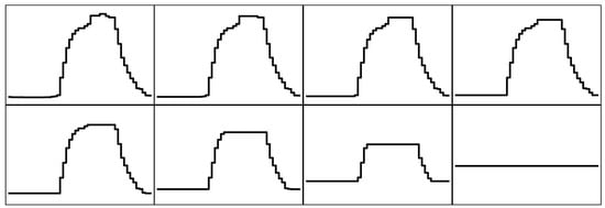
• VCM-S (Varying-coefficient model with simple basis function): our proposed method with simple basis function as in Figure 5a.
• VCM-FL (Varying-coefficient model with fused lasso): our proposed method with basis function estimated by fused lasso.
• VCM (Varying-coefficient model): statistical model in (1), but event information is not included. The method is exactly the same as in Hirose’s [14] approach.
• VCM-S-Log: VCM-S with the logarithm transformation.
• VCM-FL-Log: VCM-FL with the logarithm transformation.
• VCM-Log: VCM with the logarithm transformation.
• Sep-S (Separate regression with a simple basis function): the regression coefficients associated with the weather effect are different in each time period.
• Sep-FL: separate regression with fused lasso.
• Sep: separate regression.

As basis functions for the temperature effect and varying-coefficient models, following the work in [14], we use the cubic and cyclic B-splines for temperature effect and varying-coefficient models, respectively. When we do not employ the logarithm transformation, the candidates of regularization parameter for ridge regression, ${\lambda }_1$, are 10 grids from 1 to ${10}^{-3}$ on a log scale. Similarly, for ${\lambda }_2$, we specify 10 candidates from ${10}^3$ to 1 on a log scale. When the logarithm transformation is employed, these candidates are divided by 100; this is because average demand divided by the logarithm of average demand is approximately 100. We also specify candidates for M and Q as $M=5,10$ and $Q=5,10$. We use R package genlasso to implement the generalized lasso in VCM-FL. For NNLS implementation, we use the nnls package in R.

4.2.2. Existing Methods

To investigate the performance of our proposed method, we employ several existing machine learning techniques. We employ the SVR, lasso, Random Forest (RF), XGBoost (XGB), LightGBM (LGBM), and ARIMA as existing methods. These are frequently used in electricity forecasting. For details, refer to the literature review section, Section 2. We use R packages, randomForest, ksvm, glmnet, xgboost, and lgbm to implement the above algorithms.

For a fair comparison, the inputs/outputs used in the machine learning techniques are exactly the same as those used in our proposed method. For SVR, RF, XGBoost, LightGBM, and lasso, the forecast is based on the demand for the past T days with the same time period, average temperature, and event; that is $y_{ij}\approx f(y_{i-1,j},y_{i-2,j},\cdots ,y_{i-T+1,j},s_i,e_i)$. For the ARIMA model, we apply the ARIMA $(T,d,q)$ expressed as $y_{ij}-y_{i-d,j}=c_j+{\epsilon }_{ij}+{\sum }_{t=1}^T{\varphi }_{tj}{y}_{i-t,j}+{\sum }_{t=1}^q{\theta }_{tj}{\epsilon }_{i-t,j}+{\gamma }_j^w{s}_i+{\gamma }_j^e{e}_i$, where $c_j$, ${\varphi }_{tj}$, ${\theta }_{tj}$, ${\gamma }_j^w$, and ${\gamma }_j^e$ are model parameters and ${\epsilon }_{ij}$ ($i=1,\dots ,n$) are white noises. The above model implies that the model fitting is separately done for each time period. The detailed settings for the existing techniques, including the tuning parameter candidates and input normalization, are presented in the Supplementary Material.

In addition to the above methods, we use a hybrid model. We select the top three models that minimize the RMSE and define the forecast value by the sample mean of the three methods’ forecast values.

4.3. Result

4.3.1. Forecast Accuracy

Forecast accuracy is evaluated by the RMSE and MAPE in (3). The results for 2018 are summarized in

Table 1. Forecast accuracies of the various methods for 2018 when the event effect is incorporated into the model. The numbers corresponding to best performance are shown in bold.

	VCM-S	VCM-S-Log	Sep-S	VCM-FL	VCM-FL-Log	Sep-FL
MAPE (%)	9.4	8.3	9.4	7.9	7.7	8.0
RMSE (kW)	40.1	37.1	40.2	36.2	35.6	36.4
	Lasso	ARIMA	SVM	RF	XGB	LGBM	Hybrid
MAPE (%)	11.0	11.8	9.1	9.4	9.6	9.8	8.2
RMSE (kW)	46.5	52.3	42.1	41.3	42.7	41.7	37.1

and

Table 2. Forecast accuracies of the various methods for 2018 when the event effect is not incorporated into the model. The numbers corresponding to best performance are shown in bold.

	VCM	VCM-Log	Sep	Lasso	ARIMA	SVM	RF	XGB	LGBM
MAPE (%)	8.9	8.9	9.1	10.7	12.0	9.7	10.2	11.1	10.8
RMSE (kW)	45.5	46.1	45.8	50.3	54.1	48.8	48.2	52.8	50.4

.

Our empirical observations are as follows.

• The MAPE is generally large for all methods because this facility does not cover large-scale areas and hence has unstable electricity usage. For large-scale areas, without event information, the VCM in [14] and most machine learning techniques can result in less than 4% of MAPE, as shown in [14].
• For almost all methods, event information improves the accuracy.
• When event information is included, the VCM-FL-Log yields the best performance in both RMSE and MAPE. Basis expansion successfully captures the effects of both daily temperature and events. In addition, the logarithm transformation successfully improves accuracy when the event information is incorporated into the model.
• VCM-FL performs much better than VCM-S, implying that the event effect highly depends on the time period.
• The varying coefficient model performs slightly better than the separate regression.
• Interestingly, VCM-S provides a larger MAPE than VCM does, although the latter does not incorporate event information. A simple basis function can result in poor forecast accuracy when the event effect highly depends on the time period.
• For existing methods, SVR, RF, XGBoost, and LightGBM perform better than the lasso and ARIMA. This is probably because the lasso and ARIMA can capture only the linear relationship between temperature and demand, whereas SVR, RF, XGBoost, and LightGBM can capture the nonlinear structure.
• XGBoost and LightGBM yield similar accuracy because both are based on the gradient boosting decision tree.

4.3.2. Interpretation of Forecast Results

In Section 4.3.1, we showed that the basis function constructed using event information greatly improves accuracy. In this section, we investigate how well the fused lasso improves accuracy by interpreting the forecast results. For illustration, we focus on the demand in November 2018 shown in Figure 4. A similar tendency is observed for other months in 2018.

Figure 10 shows the forecast values estimated by VCM-FL and those estimated by VCM. Actual electricity demand is also depicted.

The result shows that the fused lasso adequately captures the large electricity demand due to the facility’s experiments. For example, on 7 November 2018, the maximum difference of two forecast values was roughly 315 kW, resulting in a 12% improvement in MAPE. Although VCM-FL generally produces larger or almost the same forecast values compared to VCM, a reversal occurs on 21 November. Interestingly, no event occurred on 21 November, and VCM-FL yielded better accuracy than VCM. We use the demand of the past four days on Wednesdays to forecast the demand, and the event occurred on the latest past two days out of the $T=4$ days (i.e., 7 and 14 November). With VCM, the electricity fluctuations caused by the events on 7 and 14 November resulted in unnecessary increase in forecast values.

The ${\widehat{y}}_{ij}$ along with ${\widehat{\mu }}_{ij}$ and ${\widehat{b}}_{ij}$ of VCM-FL and those of VCM are shown in Figure 11. At first, we find that the cyclic pattern of ${\widehat{\mu }}_{ij}$ has the same tendency over time on VCM-FL and VCM; the working time takes a larger value of ${\widehat{\mu }}_{ij}$ than the closed time. However, the curve shapes of ${\widehat{b}}_{ij}$ are completely different between the two methods. The VCM-FL can approximately capture the effect of the irregular experiments carried out in the research facility buildings. Meanwhile, the VCM cannot capture this because the event information is not included in the model.

For interpretation, we show how the fused lasso’s regularization parameter affects the basis function estimation. We estimate the basis function using the data of Thursdays from 1 January 2016 to 31 October 2018. Figure 12 shows the basis functions made with the fused lasso for various regularization parameter values ${\lambda }_2$. As the value of ${\lambda }_2$ increases, the basis function for neighboring time periods tends to take exactly equal values, thanks to the penalty $\sqrt{n}{\lambda }_2{\parallel \mathit{D}{\mathit{\gamma }}^e\parallel }_1$ in (2). In November 2018, we select ${\lambda }_2=1$, where the basis function becomes complex in daytime but takes constant value at midnight. For some other months, we select a relatively large value of ${\lambda }_2$, such as ${\lambda }_2=46.4$. In this case, the basis function is constant during the afternoon as well as at midnight. When ${\lambda }_2=464$, the basis function does not depend on the time period, resulting in exactly the same basis function as in Figure 5a.

5. Conclusions

We constructed a statistical model for forecasting the electricity demand affected by external factors, such as average temperature and irregular events. The event effect was expressed as a basis function, and several basis functions representing the event effect were presented. When the basis function could not be specified, we employed the fused lasso to automatically produce a basis function whose neighbouring time periods were likely to take exactly equal values. We applied our proposed method to the demand data of a research facility that consumed a large amount of electricity due to irregular events. The results showed that incorporating event information improved the forecast accuracy significantly in both MAPE and RMSE.

Our future research plan is to improve accuracy by incorporating variables other than daily temperature. For example, Xie et al. [80] discussed the usage of relative humidity; their empirical results showed that relative humidity has a role in improving accuracy. However, the improvement was minor when the relative humidity and temperature interaction was not included; indeed, Xie et al. [80] recommended the inclusion of eight variables related to relative humidity in the linear regression model. For our model, however, we need basis expansion, and the incorporation of eight variables would cause a significant increase in number of parameters, resulting in poor forecast accuracy. A more elaborate consideration is needed to incorporate information other than temperature into our proposed model, but this is beyond the scope of this research. We would like to take this up as a future research topic.

Another important research direction is to add other variables from a smart building, such as the number of people in the building, ventilation, electric lighting, solar shading, and network data. In particular, it is crucial to forecast solar power generation; solar gains are a decisive factor in the indoor environment. Energy consumption is calculated from the difference between actual demand and solar gains. In this case, the forecasting model would become highly complicated. It would thus be interesting to investigate how well our proposed approach based on the fused lasso performs when a complex statistical model is employed.

In this study, we evaluated the performance of our proposed procedure through the average demand deviation method. We also consider peak demand forecasting as an essential topic. For example, if a peak demand forecast with high accuracy could be achieved, it would enable us to conduct peak cut through the demand response [81], that is, managing the event. To forecast the peak demand, we need a technique specifically designed for peak demand forecasting, such as the transformation technique [82] and extreme value theory [83,84]. Another interesting future research topic is peak demand forecasting that takes irregular event information into account.

6. Patents

This research is related to Japanese patent application No. 2020-074743.

References

1. Electricity and Gas Industry Committee. Available online: https://www.meti.go.jp/shingikai/enecho/denryoku_gas/denryoku_gas/ (accessed on 8 September 2020).
2. Japan Electric Power Exchange. Available online: http://www.jepx.org/english/market/index.html (accessed on 8 September 2020).
3. Suzuki, A. An Empirical Analysis of Entrant and Incumbent Bidding in Electric Power Procurement Auctions; Waseda Global Forum: Tokyo, Japan, 2010; p. 385. [Google Scholar]
4. Vialetto, G.; Noro, M. Enhancement of a Short-Term Forecasting Method Based on Clustering and kNN: Application to an Industrial Facility Powered by a Cogenerator. Energies 2019, 12, 4407. [Google Scholar] [CrossRef] [Green Version]
5. Chapagain, K.; Kittipiyakul, S.; Kulthanavit, P. Short-Term Electricity Demand Forecasting: Impact Analysis of Temperature for Thailand. Energies 2020, 13, 2498. [Google Scholar] [CrossRef]
6. Lisi, F.; Pelagatti, M.M. Component estimation for electricity market data: Deterministic or stochastic? Energy Econ. 2018, 74, 13–37. [Google Scholar] [CrossRef]
7. Energy Information Center. Available online: http://eic-jp.org/ (accessed on 8 September 2020).
8. Iwafune, Y.; Mori, Y.; Kawai, T.; Yagita, Y. Energy-saving effect of automatic home energy report utilizing home energy management system data in Japan. Energy 2017, 125, 382–392. [Google Scholar] [CrossRef]
9. Grolinger, K.; L’Heureux, A.; Capretz, M.A.M.; Seewald, L. Energy Forecasting for Event Venues: Big Data and Prediction Accuracy. Energy Build. 2016, 112, 222–233. [Google Scholar] [CrossRef] [Green Version]
10. Grolinger, K.; Capretz, M.A.M.; Seewald, L. Energy Consumption Prediction with Big Data: Balancing Prediction Accuracy and Computational Resources. In Proceedings of the 2016 IEEE International Congress on Big Data (BigData Congress), San Francisco, CA, USA, 27 June–2 July 2016; pp. 157–164. [Google Scholar]
11. Park, J.; Park, S.; Ok, C. Optimal factory operation planning using electrical load shifting under time-based electric rates. J. Adv. Mech. Des. Syst. Manuf. 2016, 10, JAMDSM0085. [Google Scholar] [CrossRef] [Green Version]
12. Hastie, T.; Tibshirani, R. Varying-Coefficient Models. J. R. Stat. Society. Ser. B (Methodol.) 1993, 55, 757–796. [Google Scholar] [CrossRef]
13. Fan, J.; Zhang, W. Statistical Estimation in Varying-Coefficient Models. Ann. Stat. 1999, 27, 1491–1518. [Google Scholar]
14. Hirose, K. Interpretable modeling for short-and medium-term electricity load forecasting. arXiv 2020, arXiv:2006.01002. [Google Scholar]
15. Tibshirani, R.; Saunders, M.; Rosset, S.; Zhu, J.; Knight, K. Sparsity and smoothness via the fused lasso. J. R. Stat. Soc. Ser. B (Stat. Methodol.) 2005, 67, 91–108. [Google Scholar] [CrossRef] [Green Version]
16. Tibshirani, R.J.; Taylor, J. The solution path of the generalized lasso. Ann. Stat. 2011, 39, 1335–1371. [Google Scholar] [CrossRef] [Green Version]
17. Guo, Z.; Zhou, K.; Zhang, C.; Lu, X.; Chen, W.; Yang, S. Residential electricity consumption behavior: Influencing factors, related theories and intervention strategies. Renew. Sustain. Energy Rev. 2018, 81, 399–412. [Google Scholar] [CrossRef]
18. Wang, F.; Liu, L.; Yu, Y.; Li, G.; Li, J.; Shafie-Khah, M.; Catalão, J.A.P. Impact analysis of customized feedback interventions on residential electricity load consumption behavior for demand response. Energies 2018, 11, 770. [Google Scholar] [CrossRef] [Green Version]
19. Ruiz-Abellón, M.C.; Fernández-Jiménez, L.A.; Guillamón, A.; Falces, A.; García-Garre, A.; Gabaldón, A. Integration of Demand Response and Short-Term Forecasting for the Management of Prosumers’ Demand and Generation. Energies 2020, 13, 11. [Google Scholar] [CrossRef] [Green Version]
20. Hong, T.; Fan, S. Probabilistic electric load forecasting: A tutorial review. Int. J. Forecast. 2016, 32, 914–938. [Google Scholar] [CrossRef]
21. Ismail, Z.; Efendi, R.; Deris, M.M. Application of fuzzy time series approach in electric load forecasting. New Math. Nat. Comput. 2015, 11, 229–248. [Google Scholar] [CrossRef]
22. Mir, A.A.; Alghassab, M.; Ullah, K.; Khan, Z.A.; Lu, Y.; Imran, M. A Review of Electricity Demand Forecasting in Low and Middle Income Countries: The Demand Determinants and Horizons. Sustainability 2020, 12, 5931. [Google Scholar] [CrossRef]
23. Amral, N.; Ozveren, C.S.; King, D. Short term load forecasting using Multiple Linear Regression. In Proceedings of the 2007 42nd International Universities Power Engineering Conference, Brighton, UK, 4–6 September 2007; IEEE: Piscataway, NJ, USA, 2008; pp. 1192–1198. [Google Scholar]
24. Dudek, G. Pattern-based local linear regression models for short-term load forecasting. Electr. Power Syst. Res. 2016, 130, 139–147. [Google Scholar] [CrossRef]
25. Saber, A.Y.; Alam, A.K.M.R. Short term load forecasting using multiple linear regression for big data. In Proceedings of the 2017 IEEE Symposium Series on Computational Intelligence (SSCI), Honolulu, HI, USA, 27 November–1 December 2017; pp. 1–6. [Google Scholar] [CrossRef]
26. Contreras, J.; Espinola, R.; Nogales, F.J.; Conejo, A.J. ARIMA models to predict next-day electricity prices. IEEE Trans. Power Syst. 2003, 18, 1014–1020. [Google Scholar] [CrossRef]
27. Hor, C.L.; Watson, S.J.; Majithia, S. Daily load forecasting and maximum demand estimation using ARIMA and GARCH. In Proceedings of the 2006 International Conference on Probabilistic Methods Applied to Power Systems, Stockholm, Sweden, 11–15 June 2006; IEEE: Piscataway, NJ, USA, 2006; pp. 1–6. [Google Scholar]
28. Lee, C.M.; Ko, C.N. Short-term load forecasting using lifting scheme and ARIMA models. Expert Syst. Appl. 2011, 38, 5902–5911. [Google Scholar] [CrossRef]
29. Takeda, H.; Tamura, Y.; Sato, S. Using the ensemble Kalman filter for electricity load forecasting and analysis. Energy 2016, 104, 184–198. [Google Scholar] [CrossRef]
30. Engle, R.F.; Granger, C.W.; Rice, J.; Weiss, A. Semiparametric estimates of the relation between weather and electricity sales. J. Am. Stat. Assoc. 1986, 81, 310–320. [Google Scholar] [CrossRef]
31. Harvey, A.; Kopman, S.J. Forecasting Hourly Electricity Demand Using Time-Varying Splines. J. Am. Stat. Assoc. 1993, 88, 1228–1236. [Google Scholar] [CrossRef]
32. Cabrera, B.L.; Schulz, F. Forecasting Generalized Quantiles of Electricity Demand: A Functional Data Approach. J. Am. Stat. Assoc. 2017, 112, 127–136. [Google Scholar] [CrossRef] [Green Version]
33. Vilar, J.; Aneiros, G.; Raña, P. Prediction intervals for electricity demand and price using functional data. Electr. Power Energy Syst. 2018, 96, 457–472. [Google Scholar] [CrossRef]
34. Shah, I.; Lisi, F. Day-ahead electricity demand forecasting with nonparametric functional models. In Proceedings of the 2015 12th International Conference on the European Energy Market (EEM), Lisbon, Portugal, 19–22 May 2015; pp. 1–5. [Google Scholar]
35. Shah, I.; Iftikhar, H.; Ali, S.; Wang, D. Short-Term Electricity Demand Forecasting Using Components Estimation Technique. Energies 2019, 12, 2532. [Google Scholar] [CrossRef] [Green Version]
36. Tibshirani, R. Regression shrinkage and selection via the lasso. J. R. Stat. Soc. Ser. B (Methodol.) 1996, 58, 267–288. [Google Scholar] [CrossRef]
37. Ziel, F. Modelling and forecasting electricity load using Lasso methods. In Proceedings of the 2015 Modern Electric Power Systems (MEPS), Wroclaw, Poland, 6–9 July 2015; IEEE: Piscataway, NJ, USA, 2015; pp. 1–6. [Google Scholar]
38. Ziel, F.; Liu, B. Lasso estimation for GEFCom2014 probabilistic electric load forecasting. Int. J. Forecast. 2016, 32, 1029–1037. [Google Scholar] [CrossRef] [Green Version]
39. Zhang, P.; Wu, X.; Wang, X.; Bi, S. Short-term load forecasting based on big data technologies. CSEE J. Power Energy Syst. 2015, 1, 59–67. [Google Scholar] [CrossRef]
40. Chen, Y.; Xu, P.; Chu, Y.; Li, W.; Wu, Y.; Ni, L.; Bao, Y.; Wang, K. Short-term electrical load forecasting using the Support Vector Regression (SVR) model to calculate the demand response baseline for office buildings. Appl. Energy 2017, 195, 659–670. [Google Scholar] [CrossRef]
41. Elattar, E.E.; Goulermas, J.; Wu, Q.H. Electric Load Forecasting Based on Locally Weighted Support Vector Regression. IEEE Trans. Syst. Man Cybern. Part C (Appl. Rev.) 2010, 40, 438–447. [Google Scholar] [CrossRef]
42. Jiang, H.; Zhang, Y.; Muljadi, E.; Zhang, J.; Gao, W. A Short-Term and High-Resolution Distribution System Load Forecasting Approach Using Support Vector Regression with Hybrid Parameters Optimization. IEEE Trans. Smart Grid 2016, 9, 3341–3350. [Google Scholar] [CrossRef]
43. Dudek, G. Short-Term Load Forecasting Using Random Forests. In Advances in Intelligent Systems and Computing; Springer: Cham, Switzerland, 2015; Volume 323, pp. 821–828. [Google Scholar]
44. Lahouar, A.; Slama, J.B.H. Day-ahead load forecast using random forest and expert input selection. Energy Convers. Manag. 2015, 103, 1040–1051. [Google Scholar] [CrossRef]
45. Moody, J.; Christian, D. Learning with Localized Receptive Fields; Yale University, Department of Computer Science: New Haven, CT, USA, 1988. [Google Scholar]
46. Moody, J. Fast Learning in Multi-Resolution Hierarchies. In Advances in Neural Information Processing Systems; 1989; pp. 29–39. Available online: https://proceedings.neurips.cc/paper/1988/file/82161242827b703e6acf9c726942a1e4-Paper.pdf (accessed on 6 November 2020).
47. Moody, J.; Darken, C.J. Fast Learning in Networks of Locally-Tuned Processing Units. Neural Comput. 1989, 1, 281–294. [Google Scholar] [CrossRef]
48. Ortiz-Arroyo, D.; Skov, M.K.; Huynh, Q. Accurate Electricity Load Forecasting with Artificial Neural Networks. In Proceedings of the International Conference on Computational Intelligence for Modelling, Control and Automation and International Conference on Intelligent Agents, Web Technologies and Internet Commerce (CIMCA-IAWTIC’06), Vienna, Austria, 28–30 November 2005; Volume 1, pp. 94–99. [Google Scholar]
49. Karampelas, P.; Vita, V.; Pavlatos, C.; Mladenov, V.; Ekonomou, L. Design of artificial neural network models for the prediction of the Hellenic energy consumption. In Proceedings of the 10th Symposium on Neural Network Applications in Electrical Engineering (NEUREL 2010), Belgrade, Serbia, 23–25 September 2010; pp. 41–44. [Google Scholar]
50. Ekonomou, L.; Christodoulou, C.A.; Mladenov, V. A Short-Term Load Forecasting Method Using Artificial Neural Networks and Wavelet Analysis. Int. J. Power Syst. 2016, 1, 64–68. [Google Scholar]
51. Kutbatsky, V.; Sidorov, D.; Tomin, N.; Spiryaev, V. Hybrid Model for Short-Term Forecasting in Electric Power System. Int. J. Mach. Learn. Comput. 2011, 1, 138–147. [Google Scholar] [CrossRef]
52. He, W. Load Forecasting via Deep Neural Networks. Procedia Comput. Sci. 2017, 122, 308–314. [Google Scholar] [CrossRef]
53. Zhang, W.; Quan, H.; Srinivasan, D. An improved quantile regression neural network for probabilistic load forecasting. IEEE Trans. Smart Grid 2018, 10, 4425–4434. [Google Scholar] [CrossRef]
54. khantach, A.E.; Hamlich, M.; eddine Belbounaguia, N. Short-term load forecasting using machine learning and periodicity decomposition. AIMS Energy 2019, 7, 382–394. [Google Scholar] [CrossRef]
55. Marino, D.L.; Amarasinghe, K.; Manic, M. Building energy load forecasting using deep neural networks. In Proceedings of the IECON 2016—42nd Annual Conference of the IEEE Industrial Electronics Society, Florence, Italy, 24–27 October 2016; IEEE: Piscataway, NJ, USA, 2016; pp. 7046–7051. [Google Scholar]
56. Narayan, A.; Hipel, K.W. Long short term memory networks for short-term electric load forecasting. In Proceedings of the 2017 IEEE International Conference on Systems, Man, and Cybernetics (SMC), Banff, AB, Canada, 5–8 October 2017; IEEE: Piscataway, NJ, USA, 2017; pp. 2573–2578. [Google Scholar]
57. Kong, W.; Dong, Z.Y.; Jia, Y.; Hill, D.J.; Xu, Y.; Zhang, Y. Short-Term Residential Load Forecasting based on LSTM Recurrent Neural Network. IEEE Trans. Smart Grid 2017, 10, 841–851. [Google Scholar] [CrossRef]
58. Bouktif, S.; Fiaz, A.; Ouni, A.; Serhani, M.A. Multi-sequence LSTM-RNN deep learning and metaheuristics for electric load forecasting. Energies 2020, 13, 391. [Google Scholar] [CrossRef] [Green Version]
59. Zheng, H.; Yuan, J.; Chen, L. Short-term load forecasting using EMD-LSTM neural networks with a Xgboost algorithm for feature importance evaluation. Energies 2017, 10, 1168. [Google Scholar] [CrossRef] [Green Version]
60. Agrawal, R.K.; Muchahary, F.; Tripathi, M.M. Long term load forecasting with hourly predictions based on long-short-term-memory networks. In Proceedings of the 2018 IEEE Texas Power and Energy Conference (TPEC), College Station, TX, USA, 8–9 February 2018; IEEE: Piscataway, NJ, USA, 2018; pp. 1–6. [Google Scholar]
61. Abbasi, R.A.; Javaid, N.; Ghuman, M.N.J.; Khan, Z.A.; Rehman, S.U. Short Term Load Forecasting Using XGBoost. In Workshops of the International Conference on Advanced Information Networking and Applications; Springer: Cham, Switzerland, 2019; pp. 1120–1131. [Google Scholar]
62. Ju, Y.; Sun, G.; Chen, Q.; Zhang, M.; Zhu, H.; Rehman, M.U. A model combining convolutional neural network and LightGBM algorithm for ultra-short-term wind power forecasting. IEEE Access 2019, 7, 28309–28318. [Google Scholar] [CrossRef]
63. Divina, F.; Gilson, A.; Goméz-Vela, F.; García Torres, M.; Torres, J.F. Stacking ensemble learning for short-term electricity consumption forecasting. Energies 2018, 11, 949. [Google Scholar] [CrossRef] [Green Version]
64. Chen, T.; Guestrin, C. XGBoost: A scalable tree boosting system. In Proceedings of the 22nd ACM Sigkdd International Conference On Knowledge Discovery and Data Mining, San Francisco, CA, USA, 13–17 August 2016; pp. 785–794. [Google Scholar]
65. Ke, G.; Meng, Q.; Finley, T.; Wang, T.; Chen, W.; Ma, W.; Ye, Q.; Liu, T.Y. Lightgbm: A Highly Efficient Gradient Boosting Decision Tree. In Advances in Neural Information Processing Systems; 2017; pp. 3146–3154. Available online: https://proceedings.neurips.cc/paper/2017/hash/6449f44a102fde848669bdd9eb6b76fa-Abstract.html (accessed on 6 November 2020).
66. Friedman, J.H. Greedy function approximation: A gradient boosting machine. Ann. Stat. 2001, 1189–1232. [Google Scholar] [CrossRef]
67. Almalaq, A.; Edwards, G. A review of deep learning methods applied on load forecasting. In Proceedings of the 2017 16th IEEE international conference on machine learning and applications (ICMLA), Cancun, Mexico, 18–21 December 2017; IEEE: Piscataway, NJ, USA, 2017; pp. 511–516. [Google Scholar]
68. Yildiz, B.; Bilbao, J.I.; Sproul, A.B. A review and analysis of regression and machine learning models on commercial building electricity load forecasting. Renew. Sustain. Energy Rev. 2017, 73, 1104–1122. [Google Scholar] [CrossRef]
69. Mosavi, A.; Salimi, M.; Ardabili, S.F.; Rabczuk, T.; Shamshirband, S.; Varkonyi-Koczy, A.R. State of the Art of Machine Learning Models in Energy Systems, a Systematic Review. Energies 2019, 12, 1301. [Google Scholar] [CrossRef] [Green Version]
70. González-Briones, A.; Hernández, G.; Corchado, J.M.; Omatu, S.; Mohamad, M.S. Machine Learning Models for Electricity Consumption Forecasting: A Review. In Proceedings of the 2019 2nd International Conference on Computer Applications & Information Security (ICCAIS), Riyadh, Saudi Arabia, 1–3 May 2019; IEEE: Piscataway, NJ, USA, 2019; pp. 1–6. [Google Scholar]
71. Hong, T.; Gui, M.; Baran, M.E.; Willis, H.L. Modeling and Forecasting Hourly Electric Load by Multiple Linear Regression with Interactions. In Proceedings of the IEEE PES General Meeting, Providence, RI, USA, 25–29 July 2010; pp. 1–8. [Google Scholar]
72. Lawson, C.L.; Hanson, R.J. Solving Least Squares Problems; Siam: Philadelphia, PA, USA, 1995; Volume 15. [Google Scholar]
73. Chen, D.; Plemmons, R.J. Nonnegativity Constraints in Numerical Analysis. In The Birth of Numerical Analysis; World Scientific: Singapore, 2010; pp. 109–139. [Google Scholar]
74. Knight, K.; Fu, W. Asymptotics for lasso-type estimators. Ann. Stat. 2000, 28, 1356–1378. [Google Scholar]
75. Kim, S.J.; Koh, K.; Boyd, S.; Gorinevsky, D. 1 trend filtering. SIAM Rev. 2009, 51, 339–360. [Google Scholar] [CrossRef]
76. Saxena, H. Forecasting Strategies for Predicting Peak Electric Load Days. Master’s Thesis, Rochester Institute of Technology, Rochester, NY, USA, 2017; p. 72. [Google Scholar]
77. Japan Meteorological Agency. Available online: https://www.jma.go.jp/jma/indexe.html (accessed on 8 September 2020).
78. Fan, S.; Hyndman, R.J. Short-term load forecasting based on a semi-parametric additive model. IEEE Trans. Power Syst. 2011, 27, 134–141. [Google Scholar] [CrossRef] [Green Version]
79. Box, G.E.; Cox, D.R. An analysis of transformations. J. R. Stat. Soc. Ser. B (Methodol.) 1964, 26, 211–243. [Google Scholar] [CrossRef]
80. Xie, J.; Chen, Y.; Hong, T.; Laing, T.D. Relative humidity for load forecasting models. IEEE Trans. Smart Grid 2016, 9, 191–198. [Google Scholar] [CrossRef]
81. Singh, R.; Gao, P.; Lizotte, D. On hourly home peak load prediction. In Proceedings of the 2012 IEEE 3rd International Conference on Smart Grid Communications, SmartGridComm 2012, Tainan, Taiwan, 5–8 November 2012; pp. 163–168. [Google Scholar]
82. Haida, T.; Muto, S. Regression based peak load forecasting using a transformation technique. IEEE Trans. Power Syst. 1994, 9, 1788–1794. [Google Scholar] [CrossRef]
83. Li, Y.; Jones, B. The Use of Extreme Value Theory for Forecasting Long-Term Substation Maximum Electricity Demand. IEEE Trans. Power Syst. 2019, 35, 128–139. [Google Scholar] [CrossRef]
84. Jacob, M.; Neves, C.; Vukadinović Greetham, D. Forecasting and Assessing Risk of Individual Electricity Peaks; Springer Nature: Cham, Switzerland, 2020. [Google Scholar]
Figure 1. Producers and suppliers’ (PPSs’) share of electricity sales in ten areas of Japan.
Energies 13 05839 g001
Figure 2. PPSs’ electric power procurement in Japan.
Energies 13 05839 g002
Figure 3. Daily demand (solid line) and average temperature (dashed line) of a research facility in 2018. Some of the demand data values are not depicted owing to missing values or outliers.
Energies 13 05839 g003
Figure 4. Half-hourly electricity demand of a research facility in November 2018.
Energies 13 05839 g004
Figure 5. Various basis functions.
Energies 13 05839 g005
Figure 6. Daily electricity demand due to events from 1st November to 30th November 2018. The horizontal line is the threshold of 750 kW, which is used to judge whether experiments were conducted or not.
Energies 13 05839 g006
Figure 7. Schedule of experiments in research facility buildings in November 2018. Having experiments scheduled takes the value of 1, and is highlighted in yellow, and having no experiments scheduled takes the value of 0. Sundays and Saturdays are highlighted in orange and blue, respectively. The box on 23 November is highlighted in red because it is a national holiday.
Energies 13 05839 g007
Figure 8. Demand due to the event in November 2018.
Energies 13 05839 g008
Figure 9. Demand and temperature in 2018.
Energies 13 05839 g009
Figure 10. Forecast values estimated by VCM-FL and those estimated by VCM in November 2018. Actual electricity demand is also depicted.
Energies 13 05839 g010
Figure 11. Day-ahead electricity demand forecast with estimated parameters μ ^ i j and b ^ i j in November 2018.
Energies 13 05839 g011
Figure 12. Basis functions made by the fused lasso for various regularization parameters λ 2 .
Energies 13 05839 g012