Permanent-Magnet Synchronous Motor Drive System Using Backstepping Control with Three Adaptive Rules and Revised Recurring Sieved Pollaczek Polynomials Neural Network with Reformed Grey Wolf Optimization and Recouped Controller

Abstract

Owing to some nonlinear characteristics in the permanent-magnet synchronous motor (SM), such as nonlinear friction, cogging torque, wind stray torque, external load torque, and unmodeled systems, fine control performances cannot be accomplished by utilizing the general linear controllers. Thereby, the backstepping approach adopting three adaptive rules and a swapping function is brought forward for controlling the rotor motion in the permanent-magnet SM drive system to reduce nonlinear uncertainties effects. To improve the chattering phenomenon, the backstepping control with three adaptive rules using a revised recurring sieved Pollaczek polynomials neural network (RRSPPNN) with reformed grey wolf optimization (RGWO) and a recouped controller is proposed to estimate the internal collection and external collection torque uncertainties, and to recoup the smallest fabricated error of the appraised rule. In the light of the Lyapunov stability, the on-line parametric training method of the RRSPPNN can be derived through an adaptive rule. Furthermore, to obtain a beneficial learning rate and improve the convergence of the weights, the RGWO algorithm adopting two exponential-functional adjustable factors is applied to adjust the two learning rates of the weights. Then, the efficiency of the used controller is validated by test results.

1. Introduction

The permanent-magnet synchronous motors (SMs) [1] with many merits are superior to the switched reluctance motors (SRMs) and induction motors (IMs). The permanent-magnet SMs [2] can offer higher efficiency, higher power density, lower power loss, and higher robustness in comparsion with the SRMs and the IMs at the same volume. The permanent-magnet SMs have mostly adopted the field-oriented control technique owing to their easy implementation. Thereby, output torque can result in lower ripple torque in comparison with the SRMs and IMs at the same output torque. On the other hand, the permanent-magnet SMs controlled by field-oriented control [1,2], which can achieve fast four-quadrant operation, are much less sensitive to the parameter variations of the motor. Therefore, they have been widely used in many industrial applications such as robotics [1], computer numerical control (CNC) tools [2], and other mechatronics [3].

The backstepping designs [4] are befitting for a large type of linearizable nonlinear systems. Each backstepping phase can produce a novel fictitious-control design denoted by previous design phases. When the procedure ends, a feedback design can achieve the primitive design aim by utilizing the last Lyapunov function that made up by adding into the Lyapunov functions regarding all individual design phases [4]. Moreover, the backstepping control with an adaptive law has been applied in a microgyroscope [5], automatic train operation [6], aircraft flight control [7], power switcher [8], and synchronous generator [9]. Further, the backstepping control by using the modified recurrent Rogers–Szego polynomials neural network with decorated gray wolf optimization (DGWO) has been used in the permanent-magnet synchronous linear motor drive system [10]. The recouped mechanisms in these methods were absent for the estimated uncertainty. Therefore, the main aim of this paper is to improve control performances by using the proposed backstepping control with three adaptive rules using a revised recurring sieved Pollaczek polynomials neural network (RRSPPNN) with reformed grey wolf optimization (RGWO) and recouped controller.

Neural networks (NNs) have better approximation behavior in modeling [11], identification [12] and control [13] of systems. These NNs were the feedforward network structures with static mapping functions. They may not exactly respond the dynamic behavior in real time because of absent feedback loop. The recurrent NNs with feedback loop have been broadly used in the prediction of photovoltaic power output [14], an accurate electricity spot price prediction scheme [15], a photovoltaic power forecasting approach [16], and an adaptive energy management control [17] as result of higher certification and finer control performance. The primary significant property of the recurrent NN is to recollect feedback message of the foretime effect in the same neuron via its self-link. Moreover, in the general recurrent NNs, the specific self-link feedback of the hidden neuron or output neuron is in charge of recollecting the designated preceding activation of the hidden neuron or output neuron and provender to itself only. Therefore, the outputs of the other neurons have no capacity to infect the designated neuron. However, in a complex nonlinear dynamic system such as the permanent-magnet SM with nonlinear wind stray torque, flux saturation torque, cogging torque, external load torque, and interference of time-varying uncertainties, in general, seriously effect system performances. Hence, if each neuron in the recurring neural networks is considered as a state in the nonlinear dynamic systems, the self-connection feedback type is unable to approximate the dynamic systems efficiently. Due to the recurring neurons, it has certain dynamical merits over static NN and it also has been proverbially applied in photovoltaic power forecasting and electricity spot price prediction. However, these NNs take a longer time to process the online training procedure. Hence, some functional-type NNs, such as the amended recurrent Gegenbauer-functional-expansions NN [18], reformed recurrent Hermite polynomial NN [19], and mended recurrent Romanovski polynomials NN [20], have been broadly applied in the control and identification of nonlinear systems as a result of less calculation complexity. However, the adjustment mechanics of weights were not discussed in these control methods that combined with NNs. It is leads to larger error in control and identification for system. Moreover, the sieved Pollaczek polynomials [21] belong to the sieved orthogonal polynomials, according to Ismail [21]. However, the sieved Pollaczek polynomials combined with the NN have never presented in any control of nonlinear systems. Although the feedforward sieved Pollaczek polynomials neural network (SPPNN) can approximate nonlinear function, it may not be an approximated dynamic act of nonlinear uncertainties as a result of lacking a reflect loop. Because of the many benefits compared to the feedforward SPPNN, the revised recurring sieved Pollaczek polynomials neural network (RRSPPNN) control is not introduced yet for controlling the permanent-magnet SM drive system to improve the performances of the nonlinear system and computation complexity. However, the backstepping technique utilizing the RRSPPNN with error recouped agency to decrease uncertainties is thus the main motivation in this topic. Additionally, these learning rates, by utilizing acceleration factors, did not present that the convergent speed of weights is tardy.

A multi-objective grey wolf optimization (GWO) proposed by Emary et al. [22] was used to attribute the reduction of system. A GWO and conventional NN training method proposed by Mosavi et al. [23] was used in a sonar dataset category. Khandelwal et al. [24] proposed to track the programming question of transmitting network by utilizing the modified GWO. Mirjalili et al. [25] put forward a hunting mechanism of GWO to mimic the social behavior. Even though these algorithms are highly competitive and have been used in certain fields, such as distribution system [26], melanoma detection [27], and feature selection in classification [28], they have poor exploration capability and suffer from local optima stagnation. So, to improve the explorative abilities of GWO, a reformed grey wolf optimization (RGWO) algorithm adopting two exponential-functional adjustable factors is put forward as the novel method in this paper. This newly proposed algorithm makes up two revisions: Firstly, it can explore new regions in the look for space because of diverse locations assigned to the leaders. This can increase the exploration and avoid local perfect stagnation problem. Secondly, an opposition-based learning method has been used in the initial half of iterations to provide diversity among the search agents. To speed up the convergence of weights in the RRSPPNN, the RGWO with two exponential-functional adjustable factors, that is the novel method, is used to adjust the two learning rates of the weights. This novel method can prevent premature convergence and to acquire optimal learning rates with fast convergence.

The better control performance of the permanent-magnet SM drive system cannot be reached by utilizing the linear controller due to the influences of these uncertainties. To heighten robustness, the backstepping approach with three adaptive rules and a swapping function is proposed to control the permanent-magnet SM drive system to trace different periodical references. With the backstepping approach with three adaptive rules and a swapping function, the rotor position of the permanent-magnet SM drive system preserves the merits of fine transient control performance and robustness to uncertainties for the tracedifferent periodical references. Moreover, to improve the large chattering influence under uncertainties, the backstepping control with three adaptive rules by utilizing RRSPPNN with RGWO is proposed to estimate the internal bunched uncertainty and external bunched force uncertainty and the recouped controller to recoup the smallest fabricated error of the appraised rule.

Furthermore, the RGWO algorithm by using two exponential-functional adjustable factors that is applied for regulating two learning rates of the weights in the RRSPPNN is a novel method to speed up the convergence of weights in this paper. Finally, the efficiency of the backstepping control with three adaptive rules using RRSPPNN with RGWO and recouped controller is validated by some test results.

The important issue in this paper is described below. Section 2 presents the models and conformation of the permanent-magnet SM drive. Section 3 describes the backstepping control with three adaptive rules using RRSPPNN with RGWO and the recouped controller. Section 4 is the examination consequences for the permanent-magnet SM utilizing three control methods at five tested events. Section 5 is the conclusion.

2. Models and Conformation of Permanent-Magnet SM Drive

2.1. Models of Permanent-Magnet SM

For simplicity, in the three-phase $as-bs-cs$ axis coordinate frames via the Clarke and Park transformations, the voltage equations in the coordinate frames transformation from the three-phase $as-bs-cs$ axis to the $qs-ds$ axis in the permanent-magnet SM [1] are typified by

$$u_{qs}=r_s{i}_{qs}+L_{qs}d{i}_{qs}/dt+{\omega }_{es}(L_{ds}{i}_{ds}+{\lambda }_{ps})$$

(1)

$$u_{ds}=r_s{i}_{ds}+(L_{ds}d{i}_{ds}/dt+{\lambda }_{ps})-{\omega }_{es}{L}_{qs}{i}_{qs}$$

(2)

$${\omega }_{es}=p_s{\omega }_{r1}$$

(3)

$${\theta }_{es}=p_s{\theta }_{r1}$$

(4)

The electromagnetic power $P_{es}$ in the air gap as well as the electromagnetic torque $d_{e1}$ [1] can be typified by:

$$P_{es}=d_{e1}{\omega }_{es}=3p_s[{\lambda }_{ps}{i}_{qs}+(L_{ds}-L_{qs})i_{ds}{i}_{qs}]{\omega }_{es}/2$$

(5)

$$d_{e1}=3p_s[{\lambda }_{ps}{i}_{qs}+(L_{ds}-L_{qs})i_{ds}{i}_{qs}]/2$$

(6)

The dynamic equation can be typified by:

$$H_{s}d{\omega }_{r1}/dt+U_s{\omega }_{r1}=d_{e1}-d_{l1}-d_{w1}-d_{f1}-d_{c1}$$

(7)

where $u_{ds}-u_{qs}$, $i_{ds}-i_{qs}$ and $L_{ds}-L_{qs}$ stand for the $qs-ds$ axis voltages, the $qs-ds$ axis currents, and the $qs-ds$ axis inductances; $r_s$ and $p_s$ stand for the phase winding resistance and the number of pole pairs; ${\lambda }_{ps}$, ${\omega }_{es}$, and ${\omega }_{r1}$ stand for the permanent-magnet flux linkage, the electric angular speed, and the angular speed of the rotor; ${\theta }_{es}$ and ${\theta }_{r1}$ stand for the electrical angular position and the mechanical angular position of the rotor; $d_{e1}$, $d_{l1}$, $d_{f1}$, $d_{c1}$, and $d_{w1}$ stand for the electromagnetic torque, the external load torque, the flux saturation torque, the cogging torque, and the wind stray torque; $H_s$ and $U_s$ stand for total moment of inertia of permanent-magnet SM and the total viscous frictional coefficient of permanent-magnet SM.

2.2. Conformation of Permanent-Magnet SM Drive

The decoupled control technology of the permanent-magnet SM drive system is general adopting the field-oriented control (FOC) [1,2] to raise dynamic performance. The electromagnetic torque is produced by the $qs-$ axis current based on the FOC and the rotor flux is generated by the $ds-$ axis current only. When $i_{ds}$ is equal to zero and ${\lambda }_{ps}$ is equal to a constant in Equations (5) and (6), then the electromagnetic torque $d_{e1}$ will be direct ratio to $i_{qs}$ for a permanent-magnet SM drive in the closed-loop control. When the generated torque is linearly direct ratio to the $qs-$ axis current, and the $ds-$ axis rotor flux is a fixed value, the larger torque per ampere can be reached. The electromagnetic torque Equation (6) can be typified by

$$d_{e1}=3{\lambda }_{ps}{i}_{qs}^{\ast }/2=k_s{i}_{qs}^{\ast }$$

(8)

where $k_s=3p_s{\lambda }_{ps}/2$ stands for the propulsion coefficient and $i_{qs}^{\ast }$ stands for the mandate of control current. The permanent-magnet SM drive system can be predigested as $W_t(s)=1/(s{H}_s+U_s)$.

Figure 1 is the conformation of FOC permanent-magnet SM drive system, which makes up an encoder and three Hall sensors, a permanent-magnet SM, a sinusoidal pulse-width-modulation (SPWM) current control, a coordinate transformation including inverse Park and Clarke coordinate’s transformations, cos/sin generator, a speed control loop and a position control loop. The control technologies in the real-time realization are realized by utilizing the digital signal processor (DSP) controller. Rotor of permanent-magnet SM is equipped on magnet force brake that is mounted with different sizes of iron disks to change the total moment of inertia and the total viscous frictional coefficient, and to add load torque.

The FOC was realized by a digital signal processor (DSP) controller. The nominal values of used permanent-magnet SM are given as 3-phase, 2-poles, 60 Hz, 220 V, 1 kW, 2.8 A, and 3600 r/min. For the convenience of controller design, the position and speed signals in the control loop are set at 1 V = 50 rad and 1 V = 50 rad/s, respectively. The mechanical and electrical parameters of the permanent-magnet SM are given as $H_s=2.142 \times {10}^{-3 } Nm{\sec }^2=0.1071Nm\sec rad/V$, $U_s=5.86 \times {10}^{-3 } Nms/rad=0.293 Nm/V$, $r_s=2.5 \mathsf{\Omega }$, $L_{ds}=L_{qs}=4.62 mH$, $k_s=0.947 Nm/A$ by means of an open circuit test, short circuit test, blocked rotor test, and added load test. With the fulfillment of FOC [1,2,3], the permanent-magnet SM drive system can be predigested as the control block diagram portrayed in Figure 2. The perfect electromagnetic property for the drive system is hence implemented by controlling the torque current distributions to lie in the $qs-$ axis current when the d-axis current is equal to zero. Then, the torque per amp property for the drive system will generate.

3. Design of the Controller

When the permanent-magnet SM drive system with the electromagnetic torque, the wind stray torque, the flux saturation torque, the cogging torque, the parametric variations, and the external load torque disturbance is enacted, then Equation (7) is typified by

$$d{v}_s/dt=(e_s+\Delta e_s)v_s+(f_s+\Delta f_s)l_s+g_s(d_{l1}+d_{w1}+d_{f1}+d_{c1})$$

(9)

$$d{\theta }_{r1}/dt={\omega }_{r1}=v_s$$

(10)

$$b_s={\theta }_{r1}$$

(11)

where ${\theta }_{r1}$ and $v_s$ stand for the rotor position and rotor speed of the SM to be presumed bounded; $\Delta e_s$ and $\Delta f_s$ stand for two parametric uncertainties from $H_s$ and $U_s$ to be presumed bounded; $e_s={-U_s/H}_s$; $f_s={k_s/H}_s>0$; $g_s={-1/H}_s$ stand for three real numbers to be presumed bounded; $l_s=i_{qs}$ is the control propulsion of the permanent-magnet SM drive system, i.e., the propulsion current. Equation (9) can be typified by

$$d{v}_s/dt=e_s{v}_s+f_s{l}_s+d_{l1}+d_{w1}+d_{f1}+d_{c1}$$

(12)

where $w_1=\Delta e_s{v}_s$ and $w_2=\Delta f_s{d}_s$ stand for two parametric variation that are to be presumed bounded; $w_3=g_s(d_{f1}+d_{c1})$ and $w_4=g_s(d_{l1}+d_{w1})$ stand for the internal bunched uncertainty and external bunched force uncertainty to be presumed bounded.

The trace reference locus $b_m={\theta }_{m1}$ is the control goal. The design procedure is as below.

The trace error is typified by

$$e_{m1}=b_m-b_s={\theta }_{m1}-{\theta }_{r1}$$

(13)

Take differential of (13) by

$$d{e}_{m1}/dt=d{\theta }_{m1}/dt-d{\theta }_{r1}/dt=d{\theta }_{m1}/dt-v_s$$

(14)

The stabilizing function is typified by:

$${\epsilon }_{m1}=k_{m1}{e}_{m1}+d{\theta }_{m1}/dt+k_{m2}{\mu }_m$$

(15)

where $k_{m1}$ and $k_{m2}$ stand for two positive constants; ${\mu }_m=\int e_{m1}(t)dt$ stands for the integral factor.

The fictitious trace error is typified by:

$$e_{m2}=v_s-{\epsilon }_{m1}$$

(16)

Take the differential of (16) by

$$d{e}_{m2}/dt=d{v}_s/dt-d{\epsilon }_{m1}/dt=(e_s{v}_s+f_s{l}_s+w_1+w_2+w_3+w_4)-d{\epsilon }_{m1}/dt$$

(17)

where $w_1$, $w_2$, and $w_3$ stand for three unknown parameters. The estimated errors are typified by

$$e_{w1}={\widehat{w}}_1-w_1$$

(18)

$$e_{w2}={\widehat{w}}_2-w_2$$

(19)

$$e_{w3}={\widehat{w}}_3-w_3$$

(20)

where $e_{w1}$, $e_{w2}$, and $e_{w3}$ are the estimated errors; ${\widehat{w}}_1$, ${\widehat{w}}_2$, and ${\widehat{w}}_3$ are the estimated values of $w_1$, $w_2$ and $w_3$. The internal bunched uncertainty and external bunched force uncertainty $w_4$ satisfies the condition $\left|w_4\right|\le {\beta }_1$ and is to be presumed bounded.

3.1. Design of the Backstepping Control with Three Adaptive Rules and a Swapping Function

So, to design the backstepping control with three adaptive rules and a swapping function, the Lyapunov function can be typified by:

$$y_{m1}=e_{m1}^2/2+e_{m2}^2/2+e_{w1}^2/(2{\varsigma }_1)+e_{w2}^2/(2{\varsigma }_2)+e_{w3}^2/(2{\varsigma }_3)+c_{m2}{\mu }_m^2/2$$

(21)

By taking the differential of $y_{m1}$ and by utilizing Equations (14)–(20) and the integral factor ${\mu }_m=\int e_{m1}(t)dt$, Equation (21) can be typified by

$$\begin{array}{c}d{y}_{m1}/dt=e_{m1}d{e}_{m1}^{}/dt+e_{m2}d{e}_{m2}^{}/dt+e_{w1}^{}{\varsigma }_1^{-1}d{e}_{w1}^{}/dt+e_{w2}^{}{\varsigma }_2^{-1}d{e}_{w2}^{}/dt+e_{w3}^{}{\varsigma }_3^{-1}d{e}_{w3}^{}/dt+k_{m2}{\mu }_{m}d{\mu }_m^{}/dt\\ =e_{m1}(d{\theta }_{m1}/dt-v_s)+e_{m2}^{}((e_s{v}_s+f_s{l}_s+w_1+w_2+w_3+w_4)-d{\epsilon }_{m1}/dt)+e_{w1}^{}{\varsigma }_1^{-1}d{e}_{w1}^{}/dt+e_{w2}^{}{\varsigma }_2^{-1}d{e}_{w2}^{}/dt\\ +e_{w3}^{}{\varsigma }_3^{-1}d{e}_{w3}^{}/dt+k_{m2}{\mu }_{m}d{\mu }_m^{}/dt\\ =e_{m1}(-k_{m1}{e}_{m1}+{\epsilon }_{m1}-v_s)+e_{m2}^{}(e_s{v}_s+f_s{l}_s+w_1+w_2+w_3+w_4)-d{\epsilon }_{m1}/dt)+e_{w1}^{}{\varsigma }_1^{-1}d{e}_{w1}^{}/dt\\ +e_{w2}^{}{\varsigma }_2^{-1}d{e}_{w2}^{}/dt+e_{w3}^{}{\varsigma }_3^{-1}d{e}_{w3}^{}/dt+k_{m2}{\mu }_{m}d{\mu }_m^{}/dt\\ =e_{m1}(-k_{m1}{e}_{m1}-e_{m2})+e_{m2}^{}(e_s{v}_s+f_s{l}_s+w_4-d{\epsilon }_{m1}/dt)+{\widehat{w}}_1^{}{\varsigma }_1^{-1}d{\widehat{w}}_1^{}/dt+(e_{m2}^{}{w}_1-w_1^{}{\varsigma }_1^{-1}d{\widehat{w}}_1^{}/dt)\\ +{\widehat{w}}_2^{}{\varsigma }_1^{-1}d{\widehat{w}}_2^{}/dt+(e_{m2}^{}{w}_2-w_2^{}{\varsigma }_1^{-1}d{\widehat{w}}_2^{}/dt)+{\widehat{w}}_3^{}{\varsigma }_1^{-1}d{\widehat{w}}_3^{}/dt+(e_{m2}^{}{w}_3-w_3^{}{\varsigma }_1^{-1}d{\widehat{w}}_3^{}/dt)\end{array}$$

(22)

In accordance with Equation (22), the control propulsion $l_s$ in the backstepping control with three adaptive rules and a swapping function can be typified by

$$l_s=i_{qs}^{\ast }=f_s^{-1}[e_{m1}-k_{m3}{e}_{m2}-e_s{v}_s+d{\epsilon }_{m1}/dt-{\beta }_{1}sgn(e_{m2})-({\widehat{w}}_1^{}+{\widehat{w}}_2^{}+{\widehat{w}}_3^{})]$$

(23)

where $k_{m3}$ stands for a positive constant; ${\beta }_1$ stands for upper bound that is a constant, and $f_s^{-1}{\beta }_1\mathrm{sgn}(e_{m2})$ stands for a swapping function. By utilizing Equation (23), Equation (22) can be typified by:

$$\begin{array}{c}d{y}_{m1}/dt=-k_{m1}{e}_{m1}^2-c_{m3}{e}_{m2}^2-e_{m2}^{}[{\beta }_{1}sgn (e_{m2})-w_4]-e_{m2}^{}[{\widehat{w}}_1+{\widehat{w}}_2+{\widehat{w}}_3]+{\widehat{w}}_1^{}{\varsigma }_1^{-1}d{\widehat{w}}_1^{}/dt+w_1(e_{m2}^{}-{\varsigma }_1^{-1}d{\widehat{w}}_1^{}/dt)\\ +{\widehat{w}}_2^{}{\varsigma }_1^{-1}d{\widehat{w}}_2^{}/dt+w_2(e_{m2}^{}-{\varsigma }_1^{-1}d{\widehat{w}}_2^{}/dt)+{\widehat{w}}_3^{}{\varsigma }_1^{-1}d{\widehat{w}}_3^{}/dt+w_3(e_{m2}^{}-{\varsigma }_1^{-1}d{\widehat{w}}_3^{}/dt)\end{array}$$

(24)

For reaching $d{y}_{m1}(t)/dt\le 0$, three adaptive rules $d{\widehat{w}}_1/dt$, $d{\widehat{w}}_2/dt$, and $d{\widehat{w}}_3/dt$ can be typified by

$$d{\widehat{w}}_1/dt={\varsigma }_1{e}_{m2}$$

(25)

$$d{\widehat{w}}_2/dt={\varsigma }_2{e}_{m2}$$

(26)

$$d{\widehat{w}}_3/dt={\varsigma }_3{e}_{m2}$$

(27)

By utilizing Equations (25)–(27), and $\left|w_4\right|\le {\beta }_1$, then Equation (24) can be typified by

$$\begin{array}{c}d{y}_{m1}/dt=-k_{m1}{e}_{m1}^2-k_{m3}{e}_{m2}^2-e_{m2}^{}[{\beta }_{1}sgn (e_{m2})-w_4]\\ \le -k_{m1}{e}_{m1}^2-k_{m3}{e}_{m2}^2-\left|e_{m2}\right|[{\beta }_1-\left|w\right|]\\ \le -k_{m1}{e}_{m1}^2-k_{m3}{e}_{m2}^2\le 0\end{array}$$

(28)

Equation (28) shows $d{y}_{m1}(t)/dt$ to be negative semi-definite (i.e., $y_{m1}(t)\le y_{m1}(0)$), meaning that $e_{m1}$ and $e_{m2}$ are bounded. The following term is typified by

$$h_{m1}(t)=k_{m1}{e}_{m1}^2+k_{m3} e_{m2}^2=-d{q}_{m1}/dt$$

(29)

The integration of Equation (29) is typified by:

$${\int }_0^t{h}_{m1}(v)dv=q_{m1}(e_{m1}(0), e_{m2}(0))-q_{m1}(e_{m1}(t),e_{m2}(t))$$

(30)

Because $q_{m1}(e_{m1}(0), e_{m2}(0))$ is bounded and $q_{m2}(e_{m1}(t), e_{m2}(t))$ is nonincreasing and presumed bounded, then $\underset{t\to \infty }{\lim }{\int }_0^t{q}_{m1}\left(\mathrm{v}\right)d\tau <\infty$. Moreover, $d{h}_{m1}\left(t\right)/dt$ is presumed bounded, hence $h_{m1}\left(t\right)$ is a uniformly continuous function. By utilizing the Barbalat’s lemma [29,30], it can be portrayed that $\underset{t\to \infty }{\lim }{h}_{m1}(t)=0$. That is, $e_{m1}$ and $e_{m2}$ will converge to zero when $t\to \infty$. Furthermore, $\underset{t\to \infty }{\lim }{\theta }_{r1}(t)={\theta }_{m1}$ and $\underset{t\to \infty }{\lim }{v}_s=d{\theta }_{m1}/dt$. 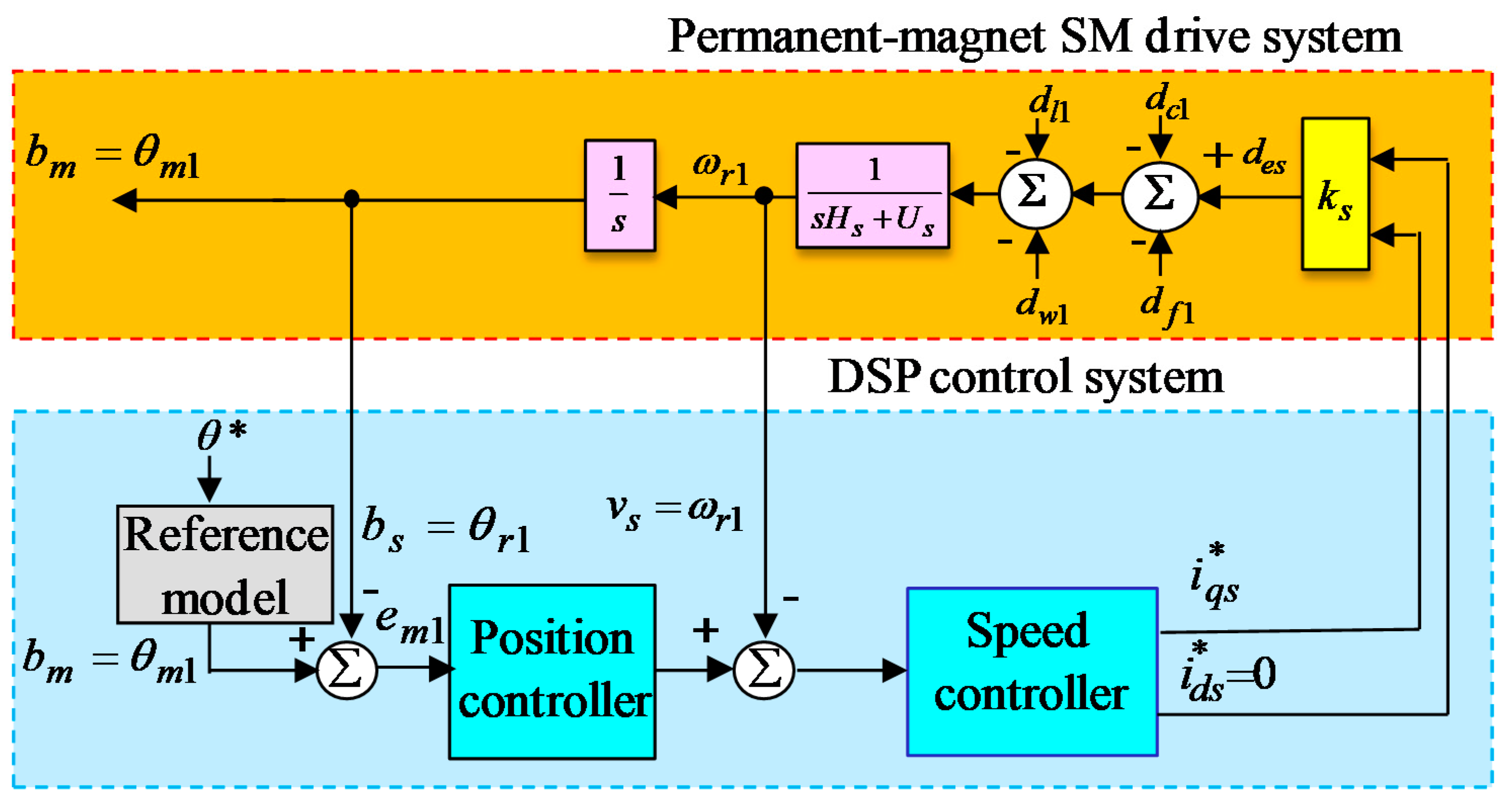The stability of the backstepping control with three adaptive rules and a swapping function can be guaranteed, and consequently, the control block diagram is portrayed in Figure 3.

3.2. Design of the Backstepping Control with Three Adaptive Rules Using RRSPPNN with RGWO and Recouped Controller

Because the internal bunched uncertainty and external bunched force uncertainty $w_4$ is unknown, and its upper bound is troublesome to be decided. The appraised value ${\widehat{w}}_4$ of the internal bunched uncertainty and external bunched force uncertainty $w_4$ is not easy to be estimated, and consequently, the revised recurring sieved Pollaczek polynomials neural network (RRSPPNN) is proposed to adapt the real value of the internal bunched uncertainty and external bunched force uncertainty $w_4$.

3.2.1. Constitution of RRSPPNN

The RRSPPNN has a three-layer constitution, with the first layer (input layer), the second layer (hidden layer 1), and the third layer (output layer) portrayed in Figure 4. The semaphore intentions in each node for each layer are explained in the following expression.

At the first layer, input semaphore and output semaphore are typified by

$$n{e}_a^1={\displaystyle \prod _c{q}_a^1(B)b_{ac}^1{o}_c^3(B-1)},o_a^1=g_a^1(n{e}_a^1)=n{e}_a^1,\hspace{1em}a=1, 2$$

(31)

where $q_1^1={\theta }_{m1}-{\theta }_{r1}=e_{m1}$ and $q_2^1=e_{m1}(1-z^{-1})=\Delta e_{m1}$ stand for the speed discrepancy and speed discrepancy alteration, respectively. B is the iteration count. $b_{ac}^1$ stands for the recurring weight through the third layer and the first layer. $o_c^3$ stands for the output of node at the third layer. The symbol $\prod$ stands for a multiply factor.

At the second layer, input semaphore and output semaphore are typified by

$$n{e}_b^2(B)={\displaystyle \sum _{a=1}^2{o}_a^1(B)}+\delta o_b^2(B-1), o_b^2=g_b^2(n{e}_b^2)=S{P}_b^{\lambda }(n{e}_b^2;q), b=0, 1,\cdots , m-1$$

(32)

where $\delta$ stands for the recurring gain at the second layer. Sieved-Pollaczek polynomials function [21,31] is adopted as the activation function. $S{P}_j^{\lambda }(q;t)$ stands for the sieved Pollaczek polynomials in the interval [−1, 1]. $S{P}_0^{\lambda }(q;t)=1$, $S{P}_1^{\lambda }(q;t)=2q$ and $S{P}_2^{\lambda }(q;t)=4q^2-1$ stand for the zero-order, first order and second order sieved Pollaczek polynomials, respectively. The sieved Pollaczek polynomials may be generated by the recurrence relation [21,31] $S{P}_{n+1}^{\lambda }(q;t)=2qS{P}_n^{\lambda }(q;t)-S{P}_{n-1}^{\lambda }(q;t)$. The symbol $\sum$ stands for a summation factor.

At the third layer, semaphore and output semaphore are typified by

$$n{e}_o^{ 3}={\displaystyle \sum _{b=0}^{m-1}{b}_{cb}^2{o}_b^2(B)}, o_c^3=g_c^3(n{e}_c^3)=n{e}_c^3,\hspace{1em}c=1$$

(33)

where $b_{cb}^2$ stands for the connecting weight through the second layer and the third layer. $g_c^3$ stands for the linear activation function. The output $o_c^3(B)$ at the third layer of the RRSPPNN can be typified by:

$$o_c^3(B)={\widehat{w}}_4(\mathsf{{\rm M}})={\mathsf{{\rm M}}}^T\mathsf{{\rm T}}$$

(34)

where $\mathsf{{\rm M}}={\left[\begin{array}{ccc}{b}_{10}^2& \cdots & b_{1, m-1}^2\end{array}\right]}^T$ and $\mathsf{{\rm T}}={\left[\begin{array}{ccc}{o}_0^2& \cdots & o_{m-1}^2\end{array}\right]}^{ T}$ stands for the weight vector at the third layer and the input vector at the third layer, respectively. The smallest fabricated error ${\phi }_{w4}$ is typified by

$$\phi { }_w=w_4-w_4({\mathsf{{\rm M}}}^{\ast })=w_4-{({\mathsf{{\rm M}}}^{\ast })}^T\mathsf{{\rm T}}$$

(35)

where ${\mathsf{{\rm M}}}^{\ast }$ stands for an ideal weight vector that reaches the smallest fabricated error. So as to make up the smallest fabricated error ${\phi }_w$, the recouped controller $x_c$ with an appraised rule is proposed. It is presumed that the small positive number $e_{w4}$ stands for greater than absolute value of ${\phi }_w$, i.e., $e_{w4}\ge \left|{\phi }_w\right|$. The Lyapunov function is typified by

$$y_{m2}=y_{m1}+{({\tilde{e}}_{w4})}^2/(2{\sigma }_1)+{(\mathsf{{\rm M}}-{\mathsf{{\rm M}}}^{\ast })}^T(\mathsf{{\rm M}}-{\mathsf{{\rm M}}}^{\ast })/(2{\gamma }_1)$$

(36)

where ${\sigma }_1$ stands for an adaptive gain. ${\tilde{e}}_{w4}={\widehat{e}}_{w4}-e_{w4}$ stands for the appraised error to be presumed bounded. By taking the derivative of $y_{m2}$ utilizing Equations (14)–(20) and the integral factor ${\mu }_m=\int e_{m1}(t)dt$, then Equation (36) is typified by

$$\begin{array}{c}d{y}_{m2}/dt=e_{m1}(-k_{m1}{e}_{m1}-e_{m2})+e_{m2}^{}(e_s{v}_s+f_s{l}_s+w_4-d{\epsilon }_{m1}/dt)+{\widehat{w}}_1^{}{\varsigma }_1^{-1}d{\widehat{w}}_1^{}/dt+w_1(e_{m2}^{}-{\varsigma }_1^{-1}d{\widehat{w}}_1^{}/dt)+{\tilde{e}}_{w4}{\sigma }_1^{-1}d{\tilde{e}}_{w4}/dt\\ +{\widehat{w}}_2^{}{\varsigma }_1^{-1}d{\widehat{w}}_2^{}/dt+w_2(e_{m2}^{}-{\varsigma }_1^{-1}d{\widehat{w}}_2^{}/dt)+{\widehat{w}}_3^{}{\varsigma }_1^{-1}d{\widehat{w}}_3^{}/dt+w_3(e_{m2}^{}-{\varsigma }_1^{-1}d{\widehat{w}}_3^{}/dt)+{\gamma }_1^{-1}{(\mathsf{{\rm M}}-{\mathsf{{\rm M}}}^{\ast })}^{T}d \mathsf{{\rm M}}/dt\end{array}$$

(37)

In accordance with Equation (37), the control propulsion $l_s={\widehat{l}}_s$ in the backstepping control with three adaptive rules by using RRSPPNN with RGWO and recouped controller can be typified by

$$l_s={\widehat{l}}_s=i_{qs}^{\ast }=f_s^{-1}[e_{m1}-c_{m3}{e}_{m2}-e_s{v}_s+d{\epsilon }_{m1}/dt-({\widehat{w}}_1^{}+{\widehat{w}}_2^{}+{\widehat{w}}_3^{})-{\widehat{w}}_4^{}(\mathsf{{\rm M}})-x_c]$$

(38)

By utilizing Equation (38), then Equation (37) can be typified by

$$\begin{array}{c}d{y}_{m2}/dt=-k_{m1}{e}_{m1}^2-k_{m3}{e}_{m2}^2+e_{m2}^{}[w_4-{\widehat{w}}_4^{}(\mathsf{{\rm M}})-x_c-({\widehat{w}}_1+{\widehat{w}}_2+{\widehat{w}}_3)]+{\widehat{w}}_1^{}{\varsigma }_1^{-1}d{\widehat{w}}_1^{}/dt+w_1(e_{m2}^{}-{\varsigma }_1^{-1}d{\widehat{w}}_1^{}/dt)+{\tilde{e}}_{w4}{\sigma }_1^{-1}d{\tilde{e}}_{w4}/dt\\ +{\widehat{w}}_2^{}{\varsigma }_1^{-1}d{\widehat{w}}_2^{}/dt+w_2(e_{m2}^{}-{\varsigma }_1^{-1}d{\widehat{w}}_2^{}/dt)+{\widehat{w}}_3^{}{\varsigma }_1^{-1}d{\widehat{w}}_3^{}/dt+w_3(e_{m2}^{}-{\varsigma }_1^{-1}d{\widehat{w}}_3^{}/dt)+{\gamma }_1^{-1}{(\mathsf{{\rm M}}-{\mathsf{{\rm M}}}^{\ast })}^{T}d \mathsf{{\rm M}}/dt\end{array}$$

(39)

By utilizing Equations (25)–(27) and ${\tilde{e}}_{w4}={\widehat{e}}_{w4}-e_{w4}$, then Equation (39) can be typified by

$$\begin{array}{c}d{y}_{m2}/dt=-k_{m1}{e}_{m1}^2-k_{m3}{e}_{m2}^2+e_{m2}^{}[w_4-w_4^{}({\mathsf{{\rm M}}}^{\ast })]-e_{m2}^{}[{\widehat{w}}_4(\mathsf{{\rm M}})-w_4^{}({\mathsf{{\rm M}}}^{\ast })]-e_{m2}^{}{x}_c+{\tilde{e}}_{w4}{\sigma }_1^{-1}d {\tilde{e}}_{w4}/dt+{\gamma }_1^{-1}{(\mathsf{{\rm M}}-{\mathsf{{\rm M}}}^{\ast })}^{T}d \mathsf{{\rm M}}/dt\\ =-k_{m1}{e}_{m1}^2-k_{m3}{e}_{m2}^2+e_{m2}^{}{\phi }_w-e_{m2}^{}[{\widehat{w}}_4(\mathsf{{\rm M}})-{\widehat{w}}_4^{}({\mathsf{{\rm M}}}^{\ast })]-e_{m2}^{}{x}_c+({\widehat{e}}_{w4}-e_{w4}){\sigma }_1^{-1}d{\widehat{e}}_{w4}/dt+{\gamma }_1^{-1}{(\mathsf{{\rm M}}-{\mathsf{{\rm M}}}^{\ast })}^{T}d \mathsf{{\rm M}}/dt\end{array}$$

(40)

3.2.2. Recouped Controller with an Adaptive Rule

To reach $d{y}_{m2}/dt\le 0$, the adaptive rule $d \mathsf{{\rm M}}/dt$, the recouped controller $x_c$, and the appraised rule $d{\widehat{e}}_{w4}/dt$ to reduce uncertainties influences can be typified by:

$$d\mathsf{{\rm M}}/dt={\gamma }_1 e_{m2} \mathsf{{\rm T}}$$

(41)

$$x_c={\widehat{e}}_{w4}\mathrm{sgn}(e_{m2})$$

(42)

$$d {\widehat{e}}_{w4}/dt={\sigma }_1\left|e_{m2}\right|$$

(43)

By substituting Equations (41)–(43) into Equation (40) and by utilizing $e_{w4}\ge \left|{\phi }_w\right|$, then Equation (40) can be typified by:

$$\begin{array}{c}d{y}_{m2}/dt=-k_{m1}{e}_{m1}^2-k_{m3}{e}_{m2}^2+e_{m2}^{}{\phi }_w-e_{m2}^{}{(\mathsf{{\rm M}}-{\mathsf{{\rm M}}}^{\ast })}^T\mathsf{{\rm T}}-e_{m2}^{}{\widehat{e}}_{w4}\mathrm{sgn}(e_{m2})+({\widehat{e}}_{w4}-e_{w4}){\sigma }_1^{-1}{\sigma }_1\left|e_{m2}\right|+{\gamma }_1^{-1}{(\mathsf{{\rm M}}-{\mathsf{{\rm M}}}^{\ast })}^T{\gamma }_1{e}_{m2}\mathsf{\Gamma }\\ =-k_{m1}{e}_{m1}^2-k_{m3}{e}_{m2}^2+e_{m2}^{}{\phi }_w-e_{w4}\left|e_{m2}\right|\\ \le -k_{m1}{e}_{m1}^2-k_{m3}{e}_{m2}^2-\left|e_{m2}\right|(e_{w4}-\left|{\phi }_w\right|)\\ \le -k_{m1}{e}_{m1}^2-k_{m3}{e}_{m2}^2\\ \le 0\end{array}$$

(44)

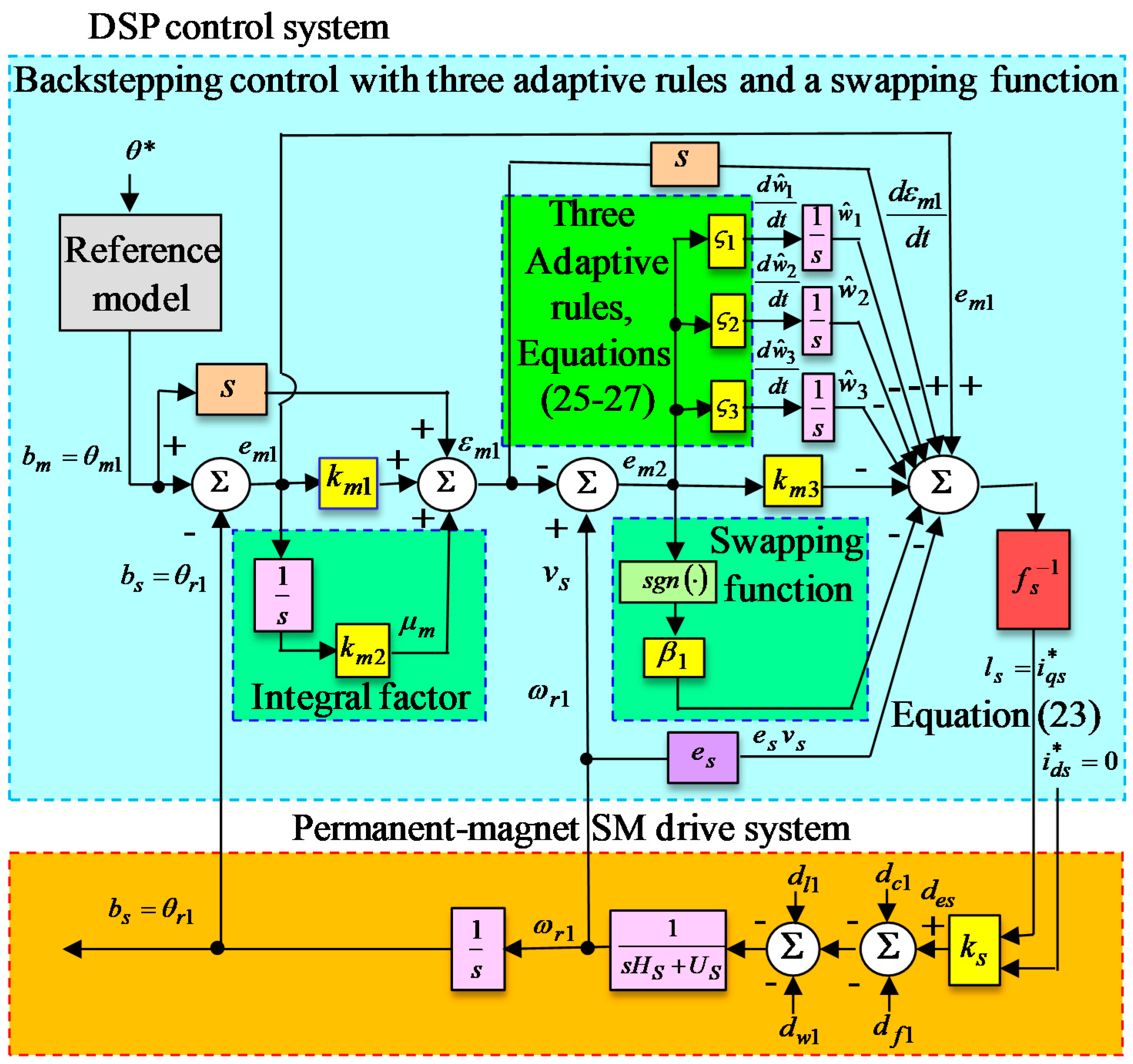
Equation (44) portrays $d{y}_{m2}(t)/dt$ to be negative semi-definite, i.e., $y_{m2}(t)\le y_{m2}(0)$, meaning that $e_{m1}$ and $e_{m2}$ are bounded. By utilizing the Barbalat’s lemma [29,30], it can be represented that $y_{m2}\left(t\right)\to 0$ at $t\to \infty$ by way of Equations (29), (30) and (44), i.e., $e_{m1}$ and $e_{m2}$ will converge to zero at $t\to \infty$. The stability of the backstepping control with three adaptive rules by using RRSPPNN with RGWO and recouped controller can be ensured and consequently the control block diagram is portrayed in Figure 5.

3.2.3. Training of the RRSPPNN

By utilizing the Lyapunov stability and the gradient descent skill with the chain rule, a training skillfulness of parameters in the RRSPPNN can be derived. The RGWO with two adjusted factors is applied to look for two better learning rates in the RRSPPNN to acquire faster convergence. The connecting weight parametric presented in Equation (41) can be typified by:

$$d{b}_{cb}^2/dt={\gamma }_1 e_{m2} o_b^2$$

(45)

A goal function that explains the online training procedure of the RRSPPNN is typified by

$$L_2=e_{m2}^2/2$$

(46)

The adaptive learning rule of the connecting weight is typified by:

$$\frac{d{b}_{cb}^2}{dt}=-{\gamma }_1\frac{\partial L_2}{\partial b_{cb}^2}=-{\gamma }_1\frac{\partial L_2}{\partial o_c^3}\frac{\partial o_c^3}{\partial n{e}_c^3}\frac{\partial n{e}_c^3}{\partial b_{cb}^2}=-{\gamma }_1\frac{\partial L_2}{\partial o_c^3}{o}_b^2$$

(47)

It is well-known that $\partial L_2/\partial o_c^3=-e_{m2}$ by way of Equations (45) and (47). Hence, the adaptive learning rule of recurring weight $b_{ac}^1$ is typified by

$$\frac{d{b}_{ac}^1}{dt}=-{\gamma }_2\frac{\partial L_2}{\partial o_c^3} \frac{\partial o_c^3}{\partial o_b^2} \frac{\partial o_b^2}{\partial n{e}_b^2} \frac{\partial n{e}_b^2}{\partial o_a^1}\frac{\partial o_a^1}{\partial n{e}_a^1} \frac{\partial n{e}_a^1}{\partial b_{ac}^1}={\gamma }_2 e_{m2} b_{cb}^{2}S{P}_b^{\lambda }(\cdot )q_a^1(B)o_c^3(B-1)$$

(48)

where ${\gamma }_2$ stands for the learning rate. To acquire better convergence, the RGWO is applied to look for two changeable learning rates in the RRSPPNN. Additionally, for improving convergence and looking for two perfect learning rates, the RGWO with two adjusted factors is proposed in this study.

3.2.4. Algorithm of Reformed Grey Wolf Optimization (RGWO)

In the RGWO, the optimization is conducted by $\alpha$, $\beta$, and $\rho$. The RGWO algorithm can be typified by:

$$H(a_1+1)=[H_1(a_1)+H_2(a_1)+H_3(a_1)]/3$$

(49)

where $H(a_1+1)=[{\gamma }_1\hspace{1em}{\gamma }_2]$ is a vector two learning rates, $H_1(a_1), H_2(a_1), H_3(a_1)$ are typified by:

$$H_1(a_1)=\left|\alpha (a_1)-R_1(a_1)\cdot [M_1(a_1)\cdot \alpha (a_1)-H(a_1)]\right|$$

(50)

$$H_2(a_1)=\left|\beta (a_1)-R_2(a_1)\cdot [M_2(a_1)\cdot \beta (a_1)-H(a_1)]\right|$$

(51)

$$H_3(a_1)=\left|\rho (a_1)-R_3(a_1)\cdot [M_3(a_1)\cdot \rho (a_1)-H(a_1)]\right|$$

(52)

where $\alpha (a_1), \beta (a_1),\rho (a_1)$ stand for the three vectors as the three best solutions. $R_1(a_1), R_2(a_1), R_3(a_1)$ and $M_1(a_1), M_2(a_1),M_3(a_1)$ can be typified by:

$$R_1(a_1)=R_2(a_1)=R_3(a_1)=2c_1(a_1){\phi }_1-d_1(a_1)$$

(53)

$$M_1(a_1)=M_2(a_1)=M_3(a_1)=2{\phi }_2$$

(54)

where ${\phi }_1$ and ${\phi }_2$ stand for two random vectors. The updated numbers of two adjusted factors $c_1(a_1)$ and $d_1(a_1)$ control the tradeoff between exploration and exploitation. Two exponential-functional adjustable factors $c_1(a_1)$ and $d_1(a_1)$ stand for the updated values at iteration according to the following presentation by:

$$c_1(a_1)=2e^{-a_1/a_{t1}}$$

(55)

$$d_1(a_1)=2e^{-a_1/a_{t2}}$$

(56)

where $a_1$ stands for the iteration number; $a_{t1}$ and $a_{t2}$ stand for the total numbers of iteration allowed for the optimization. At last, $H(a_1+1)=[{\gamma }_1\hspace{1em}{\gamma }_2]$ stands for the best solution in connection with the learning rates ${\gamma }_i(t), i=1, 2$ of the two weights in the RRSPPNN. Hence, the better numbers could be optimized by utilizing RGWO with two adjusted factors that yield two changeable learning rates for two weights to look for two perfect values and to speed-up the convergence of two weights.

4. Test Results

A block diagram of the FOC permanent-magnet SM drive system utilizing the DSP controller is portrayed in Figure 1. A photo of the examination structure is portrayed in Figure 6. The sampling time of the control program in the examination is set as 2 ms.

A DSP controller involves 18 channels of input/output (I/O) ports with 6 channels of pulse-width-modulation (PWM) ports, 6 channels of analog-digital (A/D) converters, and 2 channel encoder connective ports. The coordinate transformation in the field-oriented control (FOC) is realized by DSP controller. The used control technologies in the real-time realization by utilizing the DSP controller are composed of the core program and the sub-core interrupt service routine (SCISR) in the DSP controller as portrayed in Figure 7. In the core program, parameters and I/O initialization are processed. The interrupt time for the SCISR is set. After permitting the interruption, the core program is used to monitor control data. The SCISR with 2 msec sampling time is used for reading the rotor position of the permanent-magnet SM drive system from encoder and three-phase currents by way of A/D converter circuit, calculating reference model and position error, executing lookup table and coordinate transformation, executing the backstepping control with three adaptive rules using RRSPPNN with RGWO and recouped controller, and outputting three-phase current mandates to swap sinusoidal pulse-width-modulation (SPWM) voltage source inverter with three-sets of insulated-gate bipolar transistor (IGBT) power modules by way of the lockout-time and isolated circuits. The SPWM voltage source inverter with three-sets of IGBT power modules is carried out by SPWM control with a switching frequency of 15 kHz. Additionally, the tested bandwidth of the position control loop and the tested bandwidth of the current control loop are about 90 and 900 Hz for the permanent-magnet SM drive system under the nominal event. The proposed controllers are realized by the DSP controller. The coordinate transformation in the FOC is realized by the DSP controller. The control goal is to control the rotor to rotate 6.28 rad cyclically. Then, when the mandate is a sinusoidal reference locus, the reference is set one.

For a comparison of control performance with the four controllers, five events are provided in the experiment. The four controllers are the popular PI controller as the controller FC1, the backstepping control with three adaptive rules and a swapping function as the controller FC2, the modified recurrent Rogers–Szego polynomials neural network with DGWO [10] as the controller FC3, and the backstepping control with three adaptive rules using RRSPPNN with RGWO and recouped controller as the controller FC4. Five tested events are as follows. Event CQ1 is the nominal event at periodic step command from 0 rad to 6.28 rad. Event CQ2 is the cogging torque, the column friction torque, and the Stribeck effect torque, and the parameters variations event with 4 times the nominal value at periodic step command from 0 rad to 6.28 rad. Event CQ3 is the nominal event due to periodic sinusoidal command from −6.28 rad to 6.28 rad. Event CQ4 is the cogging torque, the column friction torque and the Stribeck effect torque and the parameters variations event with 4 times the nominal value due to periodic sinusoidal command from −6.28 rad to 6.28 rad. Event CQ5 is the adding load torque disturbance ${\tau }_{lr}=2.5 Nm$.

Two control gains of the popular PI controller as the controller FC1 are $k_{pp}=4.5,$ and $k_{ip}=k_{pp}/T_{ip}=1.8$ by using the Kronecker method to construct a stability boundary in the $k_{pp}$ and $k_{ip}$ plane [32,33,34] on the tuning of the PI controller at Event CQ1 in the position trace so as to reach fine steady-state and transient-state control responses.

Some control gains of the backstepping control with three adaptive rules and a swapping function as the controller FC2 are $k_{m1}=2.2$, $k_{m2}=2.6$, $k_{m3}=2.1$,${\varsigma }_1=0.1$, ${\varsigma }_2=0.1$, ${\varsigma }_3=0.1$, ${\beta }_1=9.1$ according to heuristic knowledge [4] at Event CQ1 in the position trace so as to reach fine steady-state and transient-state control representation.

Some control gains of the modified recurrent Rogers–Szego polynomials neural network with DGWO [10] as the controller FC3 are given as $c_{x1}=2.2$, $c_{x2}=2.6$, $c_{x3}=2.1$, ${\eta }_1=0.1$, ${\eta }_2=0.1$, ${\eta }_3=0.1$, $\gamma =0.2$, $\tau =0.1$ according to heuristic knowledge [4] at Event CQ1 in the position trace so as to reach fine steady-state and transient-state control responses. Moreover, numbers of neurons in the input layer, the hidden layer, and the output layer of the modified recurrent Rogers-Szego polynomials neural network are 2 neurons, 4 neurons and 1 neuron, respectively, so as to demonstrate the effectiveness of the controller adopting small neuron numbers. The method proposed by Lewis et al. [35] is used to initialize some parameters of the modified recurrent Rogers–Szego polynomials neural network. The adjustment process of these parameters involve a continuous reaction for the duration of the examination.

Some control gains of the backstepping control with three adaptive rules using RRSPPNN with RGWO and recouped controller as the controller FC4 are $k_{m1}=2.2$, $k_{m2}=2.6$, $k_{m3}=2.1$,${\varsigma }_1=0.1$, ${\varsigma }_2=0.1$, ${\varsigma }_3=0.1$, ${\sigma }_1=0.2$, $\delta =0.1$ according to heuristic knowledge [4] at Event CQ1 in the position trace so as to reach fine steady-state and transient-state control responses. Moreover, the number of neurons in the first layer, the second layer, and the third layer of the RRSPPNN are 2 neurons, 4 neurons, and 1 neuron, respectively, so as to demonstrate the effectiveness of the controller by adopting small neuron numbers. The method proposed by Lewis et al. [35] is used to initialize some parameters of the RRSPPNN. The adjustment process of these parameters is keeping continusly reaction in the duration of the experiments.

All of the experiments obtained by utilizing the four controllers for controlling the permanent-magnet SM drive system at five events are as follows. Figure 8a–d are rotor position responses via experiments obtained by utilizing the controllers FC1, FC2, FC3, and FC4 at Event CQ1. Figure 9a–d are rotor speed responses by utilizing the controllers FC1, FC2, FC3 and FC4 at Event CQ1. Figure 10a–d are mandate control propulsion responses by utilizing the controllers FC1, FC2, FC3, and FC4 at Event CQ1. Figure 11a–d are rotor position responses by utilizing the controllers FC1, FC2, FC3, and FC4 at Event CQ2. Figure 12a–d are rotor speed responses by utilizing the controllers FC1, FC2, FC3, and FC4 at Event CQ2. Figure 13a–d are mandate control propulsion responses by utilizing the controllers FC1, FC2, FC3, and FC4 at Event CQ2. Figure 14a–d are rotor position responses by utilizing the controllers FC1, FC2, FC3, and FC4 at Event CQ3. Figure 15a–d are rotor speed responses by utilizing the controllers FC1, FC2, FC3, and FC4 at Event CQ3. Figure 16a–d are mandate control propulsion responses by utilizing the controllers FC1, FC2, FC3, and FC4 at Event CQ3. Figure 17a–d are rotor position responses by utilizing the controllers FC1, FC2, FC3, and FC4 at Event CQ4. Figure 18a–d are rotor speed responses by utilizing the controllers FC1, FC2, FC3, and FC4 at Event CQ4. Figure 19a–d are mandate control propulsion responses by utilizing the controllers FC1, FC2, FC3, and FC4 at Event CQ4. Figure 20a–d are measured rotor position responses by utilizing the controller FC1, FC2, FC3, and FC4 at Event CQ5.

Figure 8a and Figure 14a obtained by utilizing the controller FC1 for controlling the permanent-magnet SM drive system at Event CQ1 and Event CQ3 are displayed as fine trace responses of the rotor positions. Figure 11a and Figure 17a obtained by utilizing the controller FC1 for controlling the permanent-magnet SM drive system at Event CQ2 and Event CQ4 are displayed in sluggish trace responses of the rotor position owing to bigger nonlinear disturbance. Because of inappropriate tuning gains or the degenerate nonlinear effect, the linear controller has weak robustness under bigger nonlinear disturbance.

Figure 8b, Figure 11b, Figure 14b and Figure 17b obtained by utilizing the controller FC2 for controlling the permanent-magnet SM drive system at Events CQ1, CQ2, CQ3, and CQ4 are displayed as good trace responses of the rotor positions. However, Figure 10b, Figure 13b, Figure 16b and Figure 19b are displayed as serious vibration in the control propulsions by utilizing the swapping function with large upper bound at Events CQ1, CQ2, CQ3, and CQ4. It is a well-known fact that the control propulsions with serious vibration will wear the bearing mechanism and might excite unstable system dynamics.

Figure 8c, Figure 11c, Figure 14c and Figure 17c obtained by utilizing the controller FC3 for controlling the permanent-magnet SM drive system at Events CQ1, CQ2, CQ3, and CQ4 are displayed as better trace responses of the rotor positions due to adaptive mechanism action. Figure 10c, Figure 13c, Figure 16c and Figure 19c displayed a small vibration in the control propulsions at Events CQ1, CQ2, CQ3, and CQ4. Due to the on-line adaptive adjustment of the modified recurrent Rogers–Szego polynomials neural network [10], the magnitudes of vibration in the control propulsions at Events CQ1, CQ2, CQ3, and CQ4 displayed in Figure 10c, Figure 13c, Figure 16c and Figure 19c have been slightly improved.

Figure 8d, Figure 11d, Figure 14d and Figure 17d obtained by utilizing the controller FC4 for controlling the permanent-magnet SM drive system at Events CQ1, CQ2, CQ3, and CQ4 are displayed as best trace responses of the rotor positions due to on-line adaptive mechanism action. Figure 10d, Figure 13d, Figure 16d and Figure 19d are displayed as smaller vibrations in the control propulsions at Events CQ1, CQ2, CQ3 and CQ4 due to on-line adaptive mechanism action of the RRSPPNN. Due to on-line adaptive adjustment of the RRSPPNN under bigger nonlinear disturbance the magnitudes of vibration in the control propulsions at Events CQ1, CQ2, CQ3, and CQ4 displayed in Figure 10d, Figure 13d, Figure 16d and Figure 19d have been obviously improved.

Figure 20d obtained by utilizing the controller FC4 for controlling the permanent-magnet SM drive system at Event CQ5 under load regulation is better than the controller FC1, FC2, and FC3 displayed in Figure 20a–c.

5. Discussion and Analysis

Additionally, the control performances displayed in comparsion results by using the controllers FC1, FC2, FC3, and FC4 are listed in

Table 1. Performance comparison of four controllers.

	Five Tested Events	Controller FC1
Performance		Event CQ1	Event CQ2	Event CQ3	Event CQ4	Event CQ5
Maximum error of $e_{m1}$ (rad)		0.21	0.56	0.20	0.52	3.01
Root-mean-square error of $e_{m1}$ (rad)		0.11	0.27	0.10	0.25	1.50
	Five Tested Events	Controller FC2
Performance		Event CQ1	Event CQ2	Event CQ3	Event CQ4	Event CQ5
Maximum error of $e_{m1}$ (rad)		0.19	0.36	0.18	0.37	1.57
Root-mean-square error of $e_{m1}$ (rad)		0.09	0.18	0.09	0.18	0.78
	Five Tested Events	Controller FC3
Performance		Event CQ1	Event CQ2	Event CQ3	Event CQ4	Event CQ5
Maximum error of $e_{m1}$ (rad)		0.15	0.28	0.14	0.27	1.13
Root-mean-square error of $e_{m1}$ (rad)		0.07	0.13	0.07	0.13	0.56
	Five Tested Events	Controller FC4
Performance		Event CQ1	Event CQ2	Event CQ3	Event CQ4	Event CQ5
Maximum error of $e_{m1}$ (rad)		0.10	0.19	0.10	0.18	0.75
Root-mean-square error of $e_{m1}$ (rad)		0.05	0.09	0.05	0.09	0.32

in connection with five events with some test results. The 0.21, 0.19, 0.15, and 0.10 are the maximum errors of $e_{m1}$ (rad) by utilizing the controllers FC1, FC2, FC3, and FC4 at Event CQ1, respectively. The 0.11, 0.09, 0.07, and 0.05 are the root-mean-square errors of $e_{m1}$ (rad) by utilizing the controllers FC1, FC2, FC3, and FC4 at Event CQ1, respectively. The 0.56, 0.36, 0.28, and 0.19 are the maximum errors of $e_{m1}$ (rad) by utilizing the controllers FC1, FC2, FC3, and FC4 at Event CQ2, respectively. The 0.27, 0.18, 0.13, and 0.09 are the root-mean-square errors of $e_{m1}$ (rad) by utilizing the controllers FC1, FC2, FC3, and FC4 at Event CQ2, respectively. The 0.21, 0.18, 0.14, and 0.10 are the maximum errors of $e_{m1}$ (rad) by utilizing the controllers FC1, FC2, FC3, and FC4 at Event CQ3, respectively. The 0.10, 0.09, 0.07, and 0.05 are the root-mean-square errors of errors of $e_{m1}$ (rad) by utilizing the controllers FC1, FC2, FC3, and FC4 at Event CQ3, respectively. The 0.52, 0.37, 0.27, and 0.18 are the maximum errors of $e_{m1}$ (rad) by utilizing the controllers FC1, FC2, FC3, and FC4 at Event CQ4, respectively. The 0.25, 0.18, 0.13, and 0.09 are the root-mean-square errors of $e_{m1}$ (rad) by utilizing the controllers FC1, FC2, FC3, and FC4 at Event CQ4, respectively. The 3.01, 1.57, 1.13, and 0.75 are the maximum errors of $e_{m1}$ (rad) by utilizing the controllers FC1, FC2, FC3, and FC4 at Event CQ5, respectively. The 1.50, 0.78, 0.56, and 0.32 are the root-mean-square errors of $e_{m1}$ (rad) by utilizing the controllers FC1, FC2, FC3, and FC4 at Event CQ5, respectively. The controller FC4 has smaller trace error in comparison with the controllers FC1, FC2, and FC3. The controllers FC4 indeed yields the exellent control performance from Table 1.

Furthermore, control characteristic performance comparisons in the controllers FC1, FC2, FC3, and FC4 are listed in

Table 2. Control characteristic performance comparisons of controllers.

	Four Controllers	Controller FC1	Controller FC2	Controller FC3	Controller FC4
Characteristic Performance
Vibration in control propulsion		Small	Middle	Smaller	Smallest
Dynamic response		Slow	Fast	Faster	Fastest
Ability of load regulation		Poor (maximum error as 3.01 (rad) with adding load at 6.28 (rad))	Good (maximum error as 1.57 (rad)with adding load at 6.28 (rad))	Better (maximum error as 1.13 (rad) with adding load at 6.28 (rad))	Best (maximum error as 0.09 (rad) with adding load at 6.28 (rad))
Convergence speed		Middle (traceerror response at 0.1 (rad) within 0.05 s)	Fast (traceerror respons at 0.1 (rad) within 0.04 s)	Faster (traceerror response at 0.1 (rad) within 0.03 s) (varied learning rate)	Fastest (traceerror response at 0.1 (rad) within 0.01 s) (varied learning rate)
Position traceerror		Middle	Small	Smaller	Smallest
Rejection ability for parameter disturbance		Poor	Good	Better	Best
Learning rate		None	None	Vary (optimal learning rate)	Vary (optimal learning rate)

for test results. In Table 2, various performances with regard to the control propulsion with vibration, the dynamic response, the ability of load regulation, the convergence speed, the position trace error, and the rejection ability of parameter disturbance in the controllers FC4 are superior to the controllers FC1, FC2, and FC3. Finally, the robust control performance of the controller FC4 demonstrates outstanding performance for controlling the permanent-magnet SM drive system in the trace of the periodic step and sinusoidal commands under the occurrence of parameter disturbance and load regulation due in large part to the on-line adaptive adjustment of the RRSPPNN.

6. Conclusions

The backstepping control with three adaptive rules and RRSPPNN with RGWO and recouped controller is used to determine the best values for parameters in neural network learning rules, and thereby robustness in learning control can be improved.

The main contribution of this study is as follows. Firstly, the field-oriented control has been smoothly applied to control the permanent-Magnet SM drive system to speed up the control response. Moreover, the backstepping controller with three adaptive rules and a swapping function has been smoothly derived to overcome influences under the external lumped force uncertainty disturbances in light of the Lyapunov function. Further, the backstepping control with three adaptive rules and RRSPPNN with RGWO and recouped controller to estimate the external lumped force uncertainty has been smoothly derived in the light of the Lyapunov function for diminishing the external lumped force uncertainty effect and improving the chattering phenomenon. The error recouped controller to recoup the smallest fabricated error of the error estimation law has been smoothly derived in light of the Lyapunov function. Two optimal learning rates of the RRSPPNN with two exponential-functional adjustable factors have been smoothly calculated by utilizing the RGWO algorithm to speed up the parameter’s convergence.

Finally, some control performances regarding the chattering of control propulsion, the position response, the ability of load force adjustment, the position tracing error, and the refusal ability of unknown parameters disturbance by using the backstepping control with three adaptive rules and RRSPPNN with RGWO and recouped controller are more exceptional than the popular PI controller, the backstepping control with three adaptive rules and a swapping function, and the modified recurrent Rogers–Szego polynomials neural network with DGWO [10] from Table 1 and Table 2.