Principal Component Analysis (PCA)-Supported Underfrequency Load Shedding Algorithm

Abstract

This research represents a conceptual shift in the process of introducing flexibility into power system frequency stability-related protection. The existing underfrequency load shedding (UFLS) solution, although robust and fast, has often proved to be incapable of adjusting to different operating conditions. It triggers upon detection of frequency threshold violations, and functions by interrupting the electricity supply to a certain number of consumers, both of which values are decided upon beforehand. Consequently, it often does not comply with its main purpose, i.e., bringing frequency decay to a halt. Instead, the power imbalance is often reversed, resulting in equally undesirable frequency overshoots. Researchers have sought a solution to this shortcoming either by increasing the amount of available information (by means of wide-area communication) or through complex changes to all involved protection relays. In this research, we retain the existing concept of UFLS that performs so well for fast-occurring frequency events. The flexible rebalancing of power is achieved by a small and specialized group of intelligent electronic devices (IEDs) with machine learning functionalities. These IEDs interrupt consumers only when the need to do so is detected with a high degree of certainty. Their small number assures the fine-tuning of power rebalancing and, at the same time, poses no serious threat to system stability in cases of malfunction.

1. Introduction

The worst-case scenario for an electric power system (EPS) is a long-lasting blackout [1]. To avoid such situations, frequency control mechanisms (primary, secondary, tertiary) and system integrity protection schemes (SIPS) are deployed. The primary frequency control is designed to cope with most power imbalances between supply and demand. However, when extreme situations occur, underfrequency load shedding (UFLS) and overfrequency protection for the generating units, as aspects of SIPS, are required to support frequency control. The former temporarily curtails consumption in cases of large power deficits, while the latter curtails generation in cases of large power surpluses in order to restore the balance in due time [2,3]. This is a necessity when frequency control mechanisms are not fast enough or lack sufficient power capacity. An investigation revealed that the existing (conventional) UFLS approach is often incapable of fulfilling these tasks in either a connected or an island operation [4]. Often, the electricity supply of too many consumers is interrupted, transforming the underfrequency problem into an overfrequency one, which is equally undesirable. The underlying cause of this is the insufficiency of UFLS triggering criteria (violation of preset frequency thresholds). Researchers have pursued different paths to overcome this issue, which can all be categorized into three groups [5]: (i) increasing the number of UFLS stages, which is effective only up to a certain point, as stages must not overlap in order to avoid problems caused by intentional or inherent time delays; (ii) significantly increasing the quantity of information available in order to implement better decision-making (in terms of harvesting the power of wide-area monitoring systems and, therefore, making decisions at a central location, e.g., from a control center); and (iii) suggesting thorough and often mathematically complex modifications to all the individual underfrequency relays involved in UFLS.

In contrast to the above-mentioned solutions, this research proposes a noncentralized and less abrasive approach. It involves the addition of a small number of uncoordinated intelligent electronic devices (IEDs) which act as a specialized group of underfrequency relays, the unsynchronized operation of which has several beneficial effects. The controlled quantity of consumers is limited to the size of the largest existing UFLS stage, and may be further split into a few subgroups. Due to the primary role played by the group of IEDs, we refer to it as a libero UFLS stage (L-UFLS). The term “libero” originates from volleyball vocabulary, where it describes the most skilled defensive player on the team. The L-UFLS IEDs are equipped with a special pattern recognition functionality, which makes them capable of efficiently recognizing the need for intervention and adjusting their own triggering parameters accordingly.

The significance of this solution is that it keeps the existing UFLS intact, leaving it fully capable of handling most cases of power imbalance efficiently and quickly by slowing down the fast-occurring frequency drop. The L-UFLS thresholds are set way below all conventional UFLS thresholds, and therefore, L-UFLS generally appears to be inactive. Once the need for fine-tuning of the power balance is detected by the pattern recognition algorithm, L-UFLS triggering thresholds are adjusted in order to ensure that they are triggered before the upcoming conventional UFLS stage. In this way, we avoid potential overshedding of the conventional UFLS, as our strategy allows for the disconnection of consumers in smaller bundles.

2. Methodology

The methodology is based on four procedures running online within each IED: (i) recognition of frequency-related conditions using machine learning functionalities; (ii) estimation of the forthcoming EPS frequency response a few seconds in advance through the application of a system frequency response (SFR) model; (iii) calculation of a special time characteristic, the details of which are explained in Section 2.3; and (iv) self-adjustment of the L-UFLS triggering thresholds. In the following sections, each of these procedures is discussed separately.

2.1. Recognition of Frequency-related Conditions

The process of recognizing relevant frequency-related situations can be alternatively described as a situational awareness functionality [6]. It must be highly reliable; this is the main reason why it combines several independent criteria based on principal component analysis (PCA). PCA [7,8,9] is a statistical machine learning tool that uses orthogonal transformation to convert m sets of observations described by n variables into a new, smaller principal subspace. In such a subspace, observations detected as similar form a dense cluster of points. In Figure 1b, for example, a large number of real-time measurements are transformed into the principal subspaces described by the first two (Figure 1b, right) and first three (Figure 1b, left) principal components, respectively. The same color indicates the corresponding pattern in Figure 1a. Therefore, by transforming a set of real-time measurements into the same subspace, we can easily (and very quickly) check for similarity to (but not for an exact match with) any known conditions from the database by using the k-nearest neighbor classification algorithm and a Euclidean distance metric.

Utilizing a sufficiently exhaustive database of different EPS frequency response patterns is therefore crucial. This is why numerous offline dynamic simulations were first performed and frequency-related events, illustrated in Figure 1a, captured for each simulation as a snapshot of a sliding window (representing a database entry). The appropriate selection of a sliding window length is determined by:

• the presence of intergenerator oscillations
  Since IEDs are installed in several EPS locations (substations), measured frequencies are, in general, subject to local electromechanical oscillations between the synchronous generators [10].
• the focus of interest
  In pursuing recognition of a frequency trend (e.g., decreasing, increasing, stable, etc.), wider sliding windows are required. On the other hand, if the focus is on recognizing more detailed changes (e.g., load shedding), testing indicates that window lengths of less than 200–500 ms are needed, especially considering the presence of noise in the measurements [11].

Since the oscillation frequencies are system dependent and measurement noise differs over time, two separate sliding window lengths are considered in this research: a narrow one for capturing detailed frequency changes and a wider one to identify prominent frequency trends. Each of these window types relates to its own database containing groups of snapshots, meaning that we are able to implement two independent recognition criteria. It should be emphasized that in this research, all frequency measurements contain artificially added Gaussian noise.

2.2. A Short-term Frequency-response Prediction

The SFR model [12] averages the dynamic behavior of individual synchronous machines into an equivalent-generating unit model (mutual oscillations are filtered out, but the average frequency response is retained). It assumes the domination of reheat steam turbines and neglects the impact of excitation systems, load voltage dependency, the nonlinearities of the turbine governor model and all but the largest time constants. The listed assumptions do not represent an issue, since we are only interested in a rough estimation of the EPS frequency response a couple of seconds in advance. Predicting the EPS frequency response by means of the SFR model f_SFR(t) requires the fitting of measurements f(t) in the least-squares sense:

$$\min {\displaystyle \sum _{t=t_{\mathrm{start}}}^{t_{\mathrm{end}}}{\left(f\left(t\right)-f_{\mathrm{SFR}}\left(t\right)\right)}^2}$$

(1)

The fitting involves setting the values of seven SFR model parameters [12] in the time period between t_start (detected change in power balance) and t_end (real time)—see Figure 2. It takes about 300 ms to obtain the first reliable prediction. It could be argued that this is too long, especially in networks with low inertia. However, the reader should keep in mind that, under extreme conditions, L-UFLS leaves the shedding actions to conventional relays. L-UFLS is expected to intervene only when the frequency drop is sufficiently reduced by conventional relays.

It should be noted that a real EPS involves not only reheat steam turbines, but other types of aggregates as well. These, of course, react differently to power imbalances. This is why many different SFR models and their combinations can be found in the literature [13,14]. Since the selection of an SFR model depends on constantly changing EPS characteristics, it has to be periodically reevaluated with regard to its use. However, a prediction error analysis showed that the typical prediction error of the kind of SFR described in this research was about ±120 mHz for a 5 s prediction, which was still considered accurate enough, especially if measurement noise is taken into account.

2.3. Formation of Specialized Time Characteristic

Successful estimation of the SFR model parameters (see Section 2.2) enables a rough projection of the future frequency trajectory (the shorter the reach, the smaller the prediction error) without UFLS intervention. This allows us to monitor the remaining time t_i until a forthcoming UFLS frequency threshold (denotation i) is reached in real time. If t_i cannot be determined, as when threshold violation is not expected (in the future) or the threshold has already been violated (in the past), we assign it a large default value (e.g., 30 s) for practical reasons. We are further interested in the time differences between any two consecutive thresholds:

$$\mathsf{\Delta }{t}_{\mathrm{i},\mathrm{i}+1}=t_{\mathrm{i}+1}-t_{\mathrm{i}},i=1\dots N_{\mathrm{UFLS}},$$

(2)

where N_UFLS indicates the total number of existing UFLS stages. A graphical representation of a specific time difference between stages 2 and 3 (Δt₂₃) can be found in Figure 2. Bearing these time differences in mind, we are now able to provide an illustrative example of the specialized time characteristic—see the lower part of Figure 3. This example corresponds to the two different EPS frequency responses in the upper part of Figure 3: (i) the initial high rate of change of frequency (RoCoF) in grey, and (ii) the initial low RoCoF in black. The negative Δt₁₂ (see label 1 in Figure 3) and Δt₂₃ (see label 2 in Figure 3) indicate that the frequency drop was initially too fast, so both thresholds f_TH,1 and f_TH,2 were violated before L-UFLS was needed. On the other hand, the positive Δt₃₄ (see label III in Figure 3) indicates that the frequency will violate the threshold value f_TH,3 and recover before reaching f_TH,4.

2.4. Self-Adjustment of L-UFLS Setting and Intervention

Initially, L-UFLS is inactive and the frequency thresholds (the three substages represented by grey rectangles in Figure 3 are set below all existing UFLS thresholds. Its activation is forced once the following two conditions are fulfilled: (i) a decreasing frequency trend is recognized, and (ii) any of the time differences Δt_i,i+1 in the time characteristic becomes significantly positive. As a result, L-UFLS automatically adjusts its triggering thresholds prior to the forthcoming conventional stage i (sequence of actions I, II, III and IV in Figure 3). Since we decided to have three L-UFLS substages for this research, all three were evenly spaced before the i-th UFLS stage and ready to perform the fine-tuning.

Let us examine the initial high RoCoF example in Figure 3. The first Δt which becomes significantly positive is Δt₅₆ (see label I in Figure 3). This is an indicator that the frequency will most likely never reach the conventional UFLS threshold f_TH,6, and therefore, that placing L-UFLS in front of f_TH,5 would avoid shedding the entire f_TH,5 volume. The L-UFLS substages are therefore moved upwards. After that, another Δt becomes significantly positive, namely Δt₄₅ (see label II in Figure 3). Following the same line of thinking, the L-UFLS substages are placed in front of f_TH,4. A similar move happens again with Δt₃₄ (see label III in Figure 3), which finalizes the positions of the L-UFLS substages between f_TH,2 and f_TH,3. As can be observed from the final results, this activation of the L-UFLS is sufficient for frequency stabilization and, at the same time, less load is disconnected by avoiding the activation of the fifth conventional UFLS stage.

In special cases in which the frequency forecast is delayed for whatever reason, the first of the three L-UFLS substages is set to the value of the current (real time) frequency value. Such an L-UFLS threshold setting is shown in the initial low RoCoF example in Figure 3, label IV.

2.5. L-UFLS Size and Number of Substages

Since the task of the L-UFLS is to improve the precision of power balancing, it obviously should not exceed the largest of the conventional UFLS stages. According to the regulatory requirements of the ENTSO-E interconnection, this corresponds to 10% of the total EPS load [3]. On the other hand, a single dynamic step of a smaller size than this could worsen the overall UFLS efficiency. For this reason, we chose to divide the L-UFLS into several substages, the sum of which corresponds to the largest of the conventional UFLS stages. We do not recommend a large number of substages for the following two reasons:

(1)

In general, the number of L-UFLS substages depends on the desired level of active power imbalance fine-tuning. Theoretically, full adaptability to any situation could be achieved with an infinite number of load shedding steps. However, physical devices in the real world (relays, circuit-breakers, etc.) require some time to respond to a trip signal, so a large number of substages does not necessarily mean better performance due to their possible overlap. For example, RG CE—Policy 5 [3] recommends a maximum of ten UFLS shedding steps in order to avoid such a situation.

(2)

Due to different local frequency conditions, IED detections and actions are not synchronized, nor are their triggering actions. Although this may be perceived as problematic, we believe it is actually an advantage. This is because tripping in this manner is more widely dispersed over time, and consequently, the power adjustment is more continuous compared to a coordinated approach, for which the UFLS actions are synchronized throughout the EPS. As a result, load shedding is more finely tuned and the active power is more accurately balanced. One could even consider this as a virtual introduction of several additional substages.

According to our simulations, three dynamic substages are sufficient. Furthermore, consumers applying L-UFLS could, in the future, be included in a potential demand-side response program.

2.6. IED Requirements

An IED is a microprocessor-based protection device, specialized for a specific task. Its processing speed does not have to match that of the typical protection relay, since L-UFLS activates when the frequency decay rate is moderate. It must, however, be able to perform more complex mathematical functions. Following the primary methodology steps described in Section 2.1Section 2.2Section 2.3 to Section 2.4, we list below all the features that the IED has to provide in order to participate in L-UFLS:

• Real-time frequency measurement
  This functionality is already standardized in protection relays and adopted in many other devices as well.
• Capacity to generate three independent output trip signals
  This functionality is already standardized in protection relays. These usually offer even more outputs.
• Machine learning capability
  The IED must be equipped with a PCA machine learning algorithm.
• Curve-fitting capability
  The IED must be able to perform fitting of the selected SFR model to the real-time measurements.
• Capacity to perform basic math functions for the evaluation of the expected time before violation of the static frequency limits
  The IED must be able to determine the likely time of violation of the static thresholds and their differences based on the estimated frequency response.
• Capacity to adjust its own triggering conditions
  The IED must be able to modify its own triggering settings.

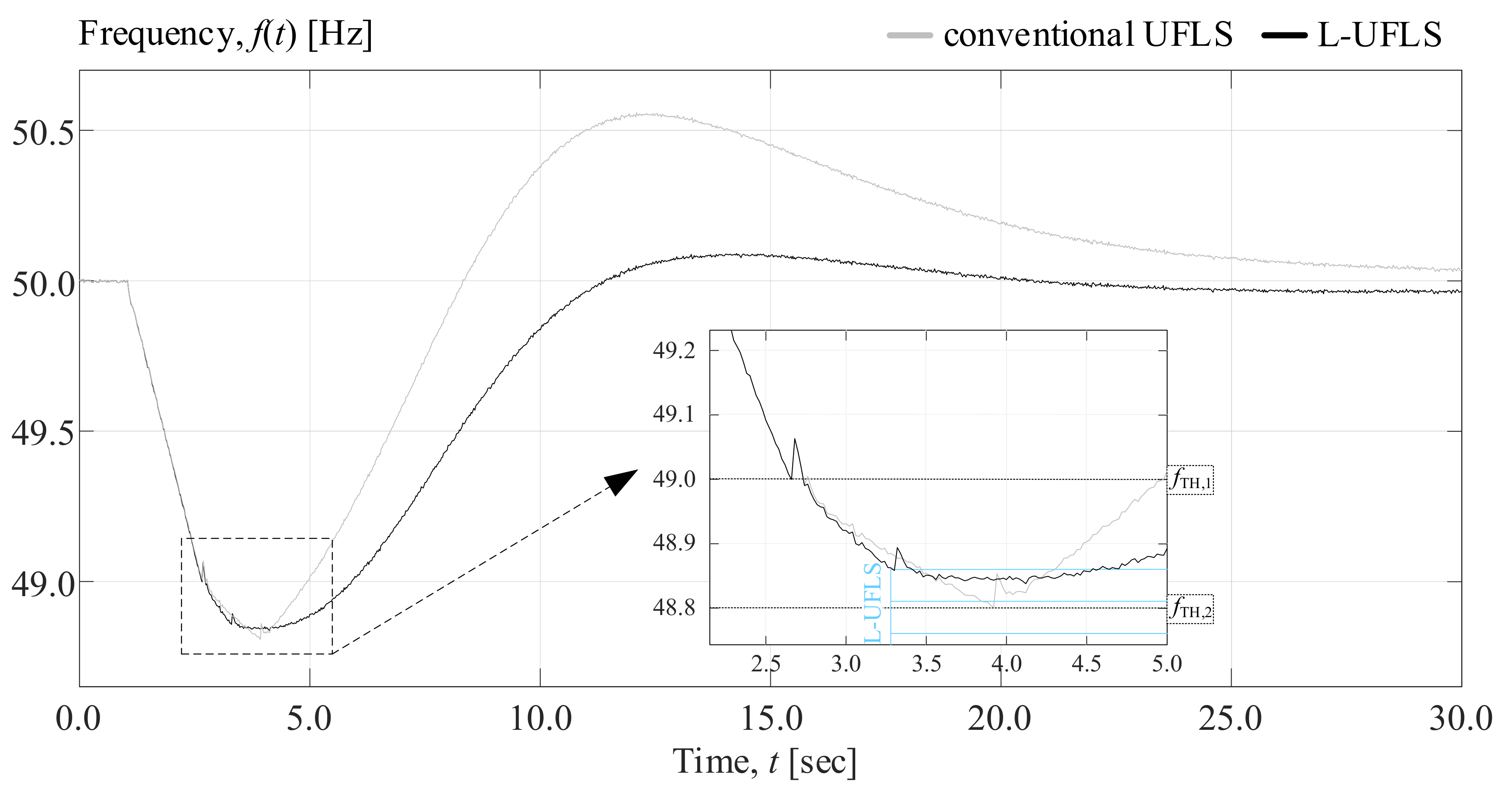
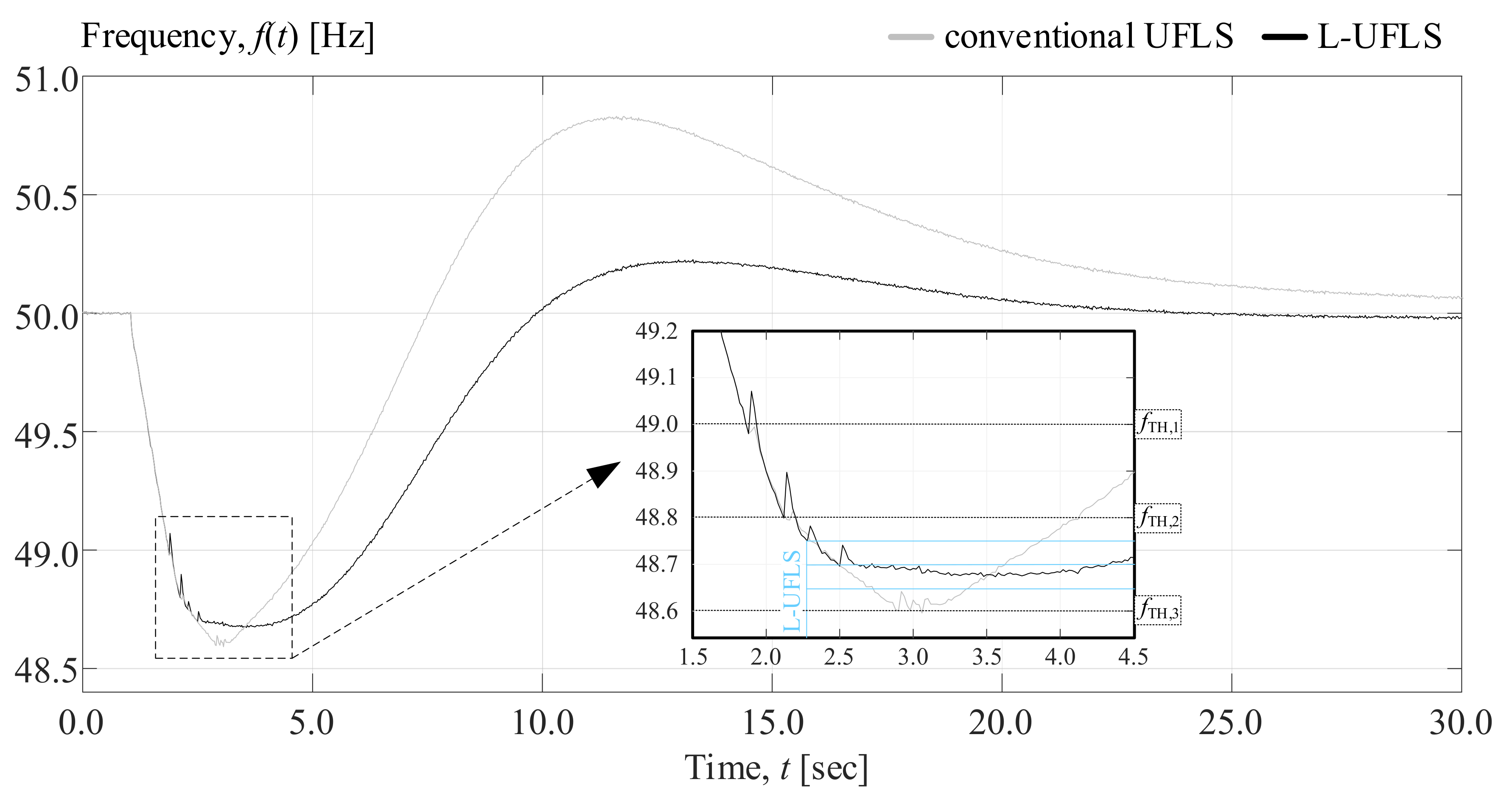
3. Case Study

The following case study involves a validated 12-generator model of a part of the 110 kV Slovenian EPS [15] and two power imbalance conditions. The PCA database was constructed from 1000 dynamic simulations and frequency recordings, differing in terms of their topology, power mismatch and power plant type and governor. Two sliding windows of different lengths (500 ms and 3000 ms) were implemented with a frequency measurement reporting rate of 20 ms (individual windows having 25 and 150 variables, respectively). The PCA similarity was evaluated using the k-nearest neighbor classification algorithm and a Euclidean distance metric. The conventional relay settings are provided in

Table 1. Conventional underfrequency load shedding (UFLS) settings.

Stage No.	1	2	3	4	5	6
fTH (Hz)	49.0	48.8	48.6	48.4	48.2	48.1
size (% of EPS loading)	10	10	10	10	10	5

. Since the largest shedding stage corresponds to 10% of the total load, L-UFLS involves the same quantity of consumers. The installed generating power was 152.45 MW. We simulated the transition to an island operation, which occurred 1.04 s after the start of the simulation.

In the first simulation (see Figure 4), the power deficit was 13% of the installed generation capacity. L-UFLS detected that conventional UFLS had successfully reduced the RoCoF to the point where it could intervene and fine-tune the power imbalance at t = 3.30 s. Therefore, L-UFLS set the first triggering threshold at 48.86 Hz. Only one, smaller substage (in addition to one static stage) was tripped, interrupting 7.6% fewer consumers than conventional UFLS tripping of two stages. Consequently, the frequency overshoot was reduced for 0.47 Hz.

In the second simulation (see Figure 5), the power deficit was 26% of the installed generation capacity. L-UFLS detected the favorable time at t = 2.28 s. Therefore, the first triggering threshold was set at 48.75 Hz. This time two substages were tripped (in addition to two static stages), but this still means that 5.5% fewer consumers were interrupted than with conventional UFLS tripping of three stages. Again, such an action reduces the overshoot, namely, for 0.60 Hz.

4. Conclusions

This paper introduces a small and specialized group of IEDs with machine learning functionalities, forming a so-called libero UFLS stage that includes a feature missing in existing UFLS. It retains the speed and robustness of conventional UFLS on the one hand, and adds flexibility on the other. Libero UFLS is split into a few equally distributed (in terms of frequency) substages, the triggering criteria of which are self-adjusted. The pattern recognition capabilities of IEDs make it possible for the libero stage to efficiently recognize the need for its intervention in terms of power imbalance fine-tuning. The number of consumers required for libero UFLS is low and can be increased gradually. Hence, possible malfunctions do not pose a serious threat to EPS stability, but can instead significantly improve the EPS frequency stability.

References

1. Matthewman, S.; Byrd, H. Blackouts: A sociology of electrical power failure. Soc. Space J. 2014, 1–25. [Google Scholar]
2. ENTSO-E. Continental Europe Operation Handbook, Appendix 1: Load-Frequency Control and Performance; ERRA: Budapest, Hungary, 2009. [Google Scholar]
3. ENTSO-E. RG CE OH—Policy 5: Emergency Operations V 3.1. Available online: https://eepublicdownloads.entsoe.eu/clean-documents/pre2015/publications/entsoe/Operation_Handbook/Policy_5_final.pdf. (accessed on 1 August 2010).
4. Alhelou, H.H.; Hamedani-Goldshan, M.E.; Njenda, C.T.; Siano, P. A Survey on Power System Blackout and Cascading Events: Research Motivations and Challenges. Energies 2019, 12, 682. [Google Scholar] [CrossRef] [Green Version]
5. Sigrist, L.; Rouco, L.; Echavarren, F.M. A review of the state of the art of UFLS schemes for isolated power systems. Electr. Power Energy Syst. 2018, 99, 525–539. [Google Scholar] [CrossRef]
6. Shahsavari, A.; Farajollahi, M.; Stewart, E.M.; Cortez, E.; Mohsenian-Rad, H. Situational Awareness in Distribution Grid Using Micro-PMU Data: A Machine Learning Approach. IEEE Trans. Smart Grid 2019, 10, 6167–6177. [Google Scholar] [CrossRef] [Green Version]
7. Jackson, J.E. A User’s Guide to Principal Components; John & Wiley, Inc.: Hoboken, NJ, USA, 1991; ISBN 978-0-471-62267-3. [Google Scholar]
8. Mohammed, S.B.; Khalid, A.; Osman, S.E.F.; Helali, R.G.M. Usage of Principal Component Analysis (PCA) in AI Applications. Int. J. Eng. Res. Technol. 2016, 5, 372–375. [Google Scholar]
9. Bishop, C.M. Pattern Recognition and Machine Learning; Springer: New York, NY, USA, 2006; ISBN 978-0387-31073-2. [Google Scholar]
10. Rudez, U.; Mihalic, R. Monitoring the First Frequency Derivative to Improve Adaptive Underfrequency Load-Shedding Scheme. IEEE Trans. Power Syst. 2011, 26, 839–846. [Google Scholar] [CrossRef]
11. ENTSO-E. Frequency Measurement Requirements and Usage—Final Version 7, RG-CE System Protection & Dynamics Sub Group; ENTSO-E: Brussels, Belgium, 2018. [Google Scholar]
12. Anderson, P.M.; Mirheydar, M. A Low-Order System Frequency Response Model. IEEE Trans. Power Syst. 1990, 5, 720–729. [Google Scholar] [CrossRef] [Green Version]
13. Huang, H.; Ju, P.; Jin, Y.; Yuan, X.; Qin, C.; Pan, X.; Zang, X. Generic System Frequency Response Model for Power Grids with Different Generations. IEEE Access 2020, 8, 14314–14321. [Google Scholar] [CrossRef]
14. Kundur, P. Power System Stability and Control; McGraw-Hill, Inc.: New York, NY, USA, 1994; ISBN 978-0070-35958-1. [Google Scholar]
15. Kopse, D.; Rudez, U.; Mihalic, R. Applying a wide-area measurement system to validate the dynamic model of a part of European power-system. Electr. Power Syst. Res. 2015, 119, 1–10. [Google Scholar] [CrossRef]
Figure 1. (a) Electric power system (EPS) frequency response patterns used during the recognition process; (b) their corresponding transformation into a principal subspace.
Energies 13 05896 g001
Figure 2. Frequency prediction and time difference estimation.
Energies 13 05896 g002
Figure 3. Illustrative example of the libero underfrequency load shedding (L-UFLS) operation.
Energies 13 05896 g003
Figure 4. Responses of conventional UFLS and L-UFLS—simulation 1.
Energies 13 05896 g004
Figure 5. Responses of conventional UFLS and L-UFLS—simulation 2.
Energies 13 05896 g005