Abstract
In order to reduce the harm of induced earthquakes in the process of geothermal energy development, it is necessary to analyze and evaluate the induced earthquake risk of a geothermal site in advance. Based on the tectonic evolution and seismogenic history around the Qiabuqia geothermal field, the focal mechanism of the earthquake was determined, and then the magnitude and direction of in-situ stress were inversed with the survey data. At the depth of more than 5 km, the maximum principal stress is distributed along NE 37°, and the maximum principal stress reaches 82 MPa at the depth of 3500 m. The induced earthquakes are evaluated by using artificial neural network (ANN) combined with in-situ stress, focal mechanism, and tectonic conditions. The predicted earthquake maximum magnitude is close to magnitude 3.
1. Introduction
As an emerging energy, geothermal energy has numerous advantages, such as clean, rich reserves, and wide distribution. As the key research of renewable clean energy in the world, the geothermal energy is divided into two types: hydrothermal and hot dry rock (HDR) geothermal [1]. The HDR is usually buried at a depth of 3–10 km from the ground, and its temperature is between 150–650 °C [2]. In order to extract the energy contained in HDR, it is usually necessary to transform it into high permeability rock mass by artificial fracturing to meet the requirements of an enhanced geothermal system (EGS) [3]. The EGS drilled two or more parallel or nearly parallel wells in the HDR region, and formed a fracture network between wells by hydraulic fracturing, and then formed hydraulic circulation between wells to achieve the purpose of developing and utilizing geothermal energy [4].
However, the induced earthquake has become a problem that cannot be ignored in EGS [5], especially after the 5.4 earthquake occurred in Pohang, Korea on 5 November 2017. It is not only in the process of hydraulic fracturing, but also in the later stage of hydraulic circulation heat recovery, which may cause the occurrence of an earthquake, such as the Geysers geothermal field, USA [6,7]; Cooper Basin, Australia [8]; Berlín, El Salvador [9]; Soultz-sous-Forêts, France [10]; Basel Deep Heat Mining [11], Switzerland, etc.
At present, hot dry rocks have been discovered in Qiabuqia area in the northeast of Qinghai Tibet Plateau. The temperature can reach 236 °C at 3705 m depth. The Qiabuqia geothermal region is located in the Gonghe Basin in Northwest China [12,13]. The site is nearly elliptical, covering an area of 246.9 km2. The total resource is equivalent to more than 200 billion tons of standard coal. To establish the EGS in the Qiabuqia area and reduce the damage caused by induced earthquakes, the in-situ stress state, historical distribution of earthquakes, and tectonic conditions are investigated.
According to the survey data, the in-situ stress inversion of the Qiabuqia geothermal field is carried out, and the historical seismic data of the area are collected to obtain the main focal mechanism of the area. At the same time, combined with the evolution of geological structure in the Qiabuqia area, the risk assessment of induced earthquakes in the process of geothermal energy exploitation in this area is carried out by using an artificial neural network (ANN).
In the fields of pattern recognition, automatic control, prediction, and estimation, ANN has successfully solved many practical problems that are difficult to be solved by modern computers, and shows good intelligent characteristics [14]. The ANN model mainly considers the topology structure of network connection, the characteristics of neurons, and learning rules. At present, there are nearly 40 kinds of neural network models, such as back-propagation network, perceptron, self-organizing map, Hopfield network, Boltzmann machine, and adaptive resonance theory. According to the topology of the connection, the neural network model can be divided into forward network and feedback network.
Artificial neural network is widely used in shallow geothermal systems. Hikmet Esen et al. [15,16] used ANN to predict the performance of a vertical ground coupled heat pump (VGCHP) system and horizontal ground coupled heat pump (GCHP) system. On the basis of ANN, Gang et al. [17] predicted the heat production effect of hybrid ground source heat pump (HGSHP) system and its controlled ground heat exchanger (GHE). Zhou et al. [18] studied the prediction of EGS production temperature by artificial neural network. In the aspect of earthquake prediction, the artificial neural network model also has been applied to a certain extent. Zakeri, NSS et al. [14] presented an application of a supervised feed forward artificial neural network that is trained on the basis of genetic algorithm (GA). The network model is used for predicting the magnitude of earthquakes in the North Tabriz Fault (NTF) Northwest Iran. Zamani, A et al. [19] used ANN model to analyze the spatial and temporal distribution of seismicity activity.
In this paper, we integrate the survey data of the Qiabuqia geothermal field with the collected tectonic evolution and seismogenic history of the field, and inversed the in-situ stress state of the Qiabuqia area, and determined the focal mechanism of the earthquake. Then, the ANN model is used to predict and evaluate the induced earthquakes in the process of EGS development in the Qiabuqia geothermal field to minimize the damage caused by induced earthquakes.
2. Overview of Qiabuqia Geothermal Field
Located in the east of Gonghe Basin in Northwest China, the Qiabuqia geothermal field is one of the three identified geothermal fields in Gonghe Basin. The total area of geothermal field is more than 790 km2, and the area of the Qiabuqia geothermal field is 246.9 km2 [20], as shown in Figure 1.
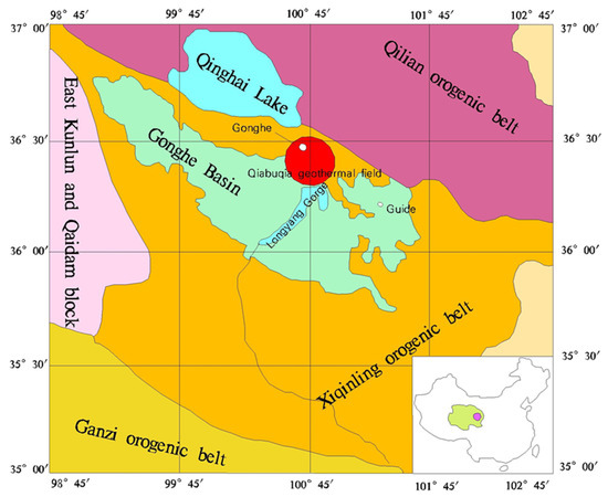
Figure 1.
Location of the Qiabuqia geothermal field.
Gonghe Basin locate in the important node area where many blocks (such as West Qinling, Qilian Mountains, East Kunlun, and Qaidam blocks) of the Central Orogenic Belt. There are two periods of magmatic activity in the area, namely, the Variscan and Indosinian periods. The magmatic activities are strictly controlled by the Daotanghe Jiangxi Gou (deep) fault. The most intense tectonic movement in the area may occur at the end of Triassic or later. The movement has basically shaped the east–west structural belt. Since the late Cenozoic, the deformation of the whole Qinghai Tibet Plateau, especially in the northeast margin, is mainly characterized by NE crustal shortening and clockwise rotation [21].
Gonghe Basin is located in the junction area of East Kunlun, West Qinling, and South Qilian. Its tectonic location is special, and its tectonic evolution has the characteristics of “two periods and five stages”: trigeminal rift structure in Early Paleozoic, rift dynamic background transformation in Late Paleozoic, continuous collision in early Middle Triassic, collisional orogeny in Late Triassic, and mountain formation of Nanshan uplift in Pliocene. Finally, Nanshan uplifted rapidly and the United basin was decomposed into two independent basin units, Qinghai Lake fault basin and Gonghe fault basin, forming the present tectonic framework [22], as shown in Figure 2.
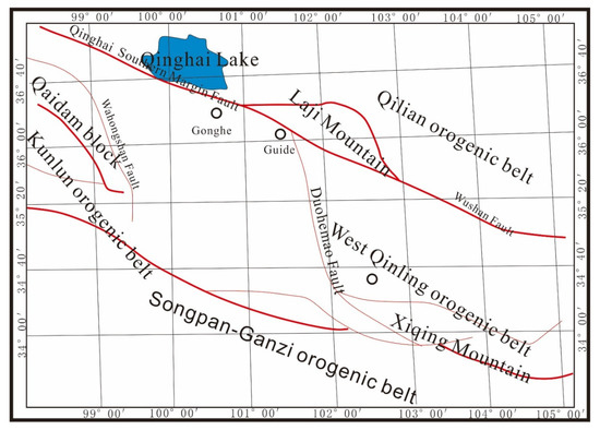
Figure 2.
Tectonic map of Gonghe and its surrounding areas.
3. Focal Mechanism Analysis
Focal mechanism is the most widely used basic data in the study of Crustal Dynamics [23]. Due to the complexity of seismotectonics and focal conditions, as well as the random error of observation data, the source information obtained from a single earthquake can only reflect the stress activity state of the point, but not the crustal stress field in a certain area [24]. However, a great many of statistical results of focal mechanism solutions can basically reflect the basic features of tectonic stress field in the study region [25]. In the same way, moderate and strong earthquakes, especially strong earthquakes, have high seismic energy and large earthquake volume. Their focal mechanism solutions can well reflect the large regional crustal stress field [26,27].
In this study, we have collected all the earthquakes since 1950 in the area where the site is located: 98.5°–102.5° E, 35°–37.5° N. There were 97 earthquakes with Ms ≥ 3.0 and 13 earthquakes with Ms ≥ 5.0. Then, the mechanical mechanism of 13 earthquakes with detailed data records was analyzed, and the location relationship between them and the well site is shown in the Figure 3.
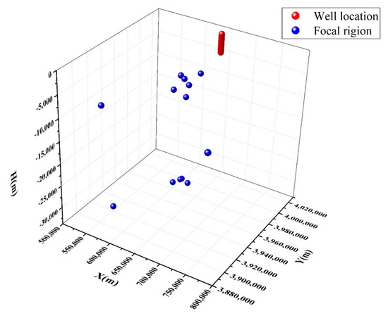
Figure 3.
Focal region spatial distribution.
Seismic faults are usually described by three parameters: strike φS, dip angle δ, and slip angle λ. Strike φS: direction of intersecting plane with horizontal plane. Direction determination: along the strike, the hanging wall of the fault is on the right. The strike direction is represented by the angle from the north clockwise needle amount to the strike direction, with 0° ≤ φS < 360°. Dip angle δ: the angle between fault plane and horizontal plane, with 0° < δ ≤ 90°. Slip angle λ: measured on the fault plane, the angle from anticlockwise direction to slip direction is positive, and the angle from clockwise needle to slip direction is negative. The slip direction refers to the movement direction of hanging wall relative to footwall, with −180° < λ ≤ 180°. Strike φS and dip angle δ are the geometric parameters of faults, which determine the occurrence of faults; the slip angle λ is the motion parameter of faults, from which all kinds of motion types of faults can be described, as shown in Figure 4 and Figure 5.
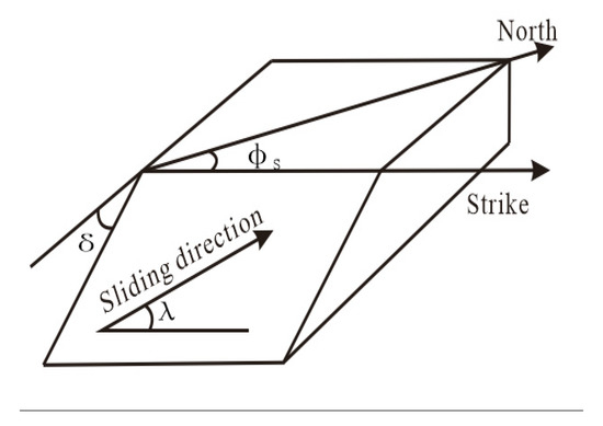
Figure 4.
Definition of source parameters.
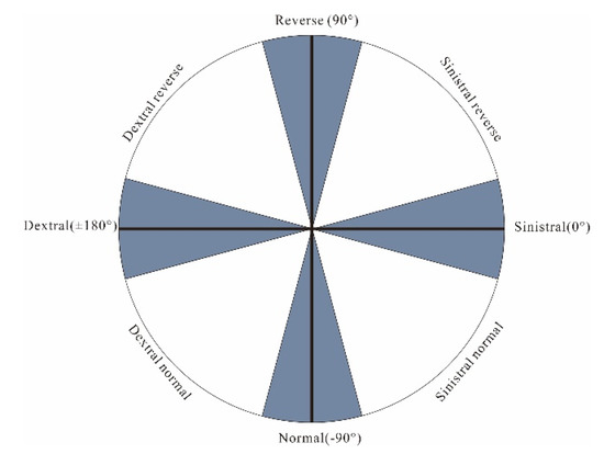
Figure 5.
Fault property determination.
According to the point source double couple mode, the initial motion direction of the far-field displacement can be calculated as a regular quadrant distribution. The distribution of the initial motion direction on the projection plane of the source sphere can be obtained from the station records in different directions relative to the source, and the positions of the principal stress axis and 2 nodal planes are given, as shown in Figure 6.
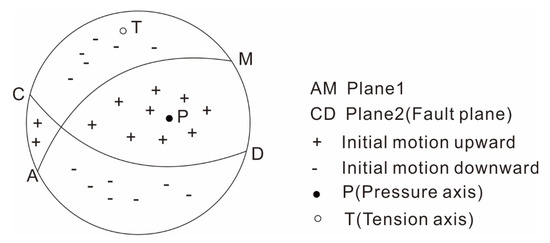
Figure 6.
Beach ball model of focal mechanism.
Table 1 and Figure 7 show the focal mechanism solutions and location distribution of 13 earthquakes with Ms ≥ 5.0. According to this information, we can carry out the analysis and inversion of the magnitude and orientation of in-situ stress.

Table 1.
Seismic information statistics (Ms ≥ 5.0).
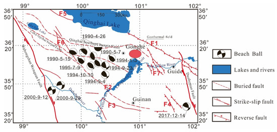
Figure 7.
Distribution of focal mechanism.
4. Analysis of In-Situ Stress Field
The Qiabuqia geothermal field is located in the Gonghe Basin, which is located in the northeast of Qinghai Tibet Plateau, with Nanshan Mountain in the north, ELa mountain in the northwest, and Waligong mountain in the East 20. The boundary of the whole basin is very irregular, and the plane is an irregular quadrilateral extending in NW direction. Therefore, the situation of in-situ stress field is more complex, so the in-situ stress field of geothermal site should be determined comprehensively from different angles.
4.1. Determination of In-Situ Stress Direction
4.1.1. Determination of In-Situ Stress Direction Based on Joint Fracture Statistics
For rocks with less weathering and erosion, most of the joints and fissures are produced by the tectonic action of the in-situ stress field [28]. These fissures constitute the dominant fissures of the rock mass joint fissures, which have strong statistical laws. The rest of the fractures are mainly produced by weathering erosion or diagenesis. These fissures are usually disordered and have no statistical rules. Through the reconstruction of three-dimensional fractures, we find that most of the joints and fissures are straight and run through each other, which are typical conjugate shear joints.
In this investigation of regional in-situ stress and the important means to deduce the distribution of deep fractures in the stratum is to carry out the statistics of joints and fissures, with a total of 80 joints and fissures. Based on the investigation results, 3D reconstruction of joints and fissures is carried out, as shown in Figure 8. Through the rose diagram of joints and fissures, the dominant orientation of joints and fissures is studied, and the situation of in-situ stress direction in the study region is obtained.
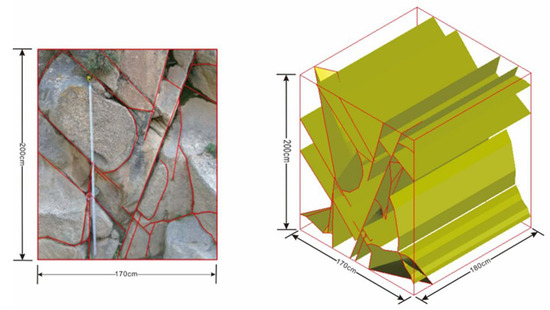
Figure 8.
Three-dimensional fracture reconstruction.
All the joints and fissures in the survey area are counted and the rose diagram of joints and fissures in the survey area is made, as shown in Figure 9 and Figure 10. According to the stress mechanism of shear joints, the maximum principal stress direction in granite in this survey area is about NE 77° and dip angle is 75° and the maximum principal stress direction in mudstone and sandstone is about NE 73° and dip angle is 82°, respectively. Based on the field survey results of granite and mudstone, the joint fracture survey shows that the maximum principal stress is about NE 73° to 77° and the maximum principal stress dip angle is 75° to 82°. At the same time, we have made statistical analysis on the joints and fissures of each survey point, and the analysis results are shown in Table 2.
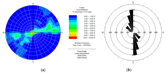
Figure 9.
Statistical results of joints and fissures in granite. (a) Iso-density map; (b) Rose diagram of joint strike.
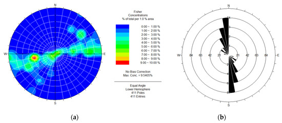
Figure 10.
Statistical results of joints and fissures in mudstone and sandstone. (a) Iso-density map; (b) Rose diagram of joint strike.
Table 2.
Principal stress direction of joint and fissure investigation points.
However, we have carried out Kriging interpolation analysis on joint fracture results to obtain the variation trend of regional in-situ stress. Based on the theory of regional variogram, the variogram and unbiased estimation of minimum variance are used to establish and solve the equations of interpolation coefficients. The statistical results show that the maximum principal stress is distributed in NE 60°–84 ° in the region, showing an increasing trend from east to west, increasing from north to south. The maximum principal stress is distributed along NE 72° and dip angle of maximum principal stress is 81.5° in the geothermal field.
4.1.2. Determination of In-Situ Stress Direction Based on Structural Analysis of Small Faults
In this field survey, the occurrence and scratch analysis of regional faults near Tulin, Ayihai ditch, and north bank of Longyangxia reservoir are carried out. According to Anderson fault stress model, the direction of in-situ stress distribution in small areas is analyzed first, and then the fault structures in large areas of Gonghe Basin are studied through data.
The faults in the survey area are modeled as shown in the Figure 11. These small faults are small in scale and extend from several meters to tens of meters. Then the in-situ stress direction is assigned to each fault point, and the regional in-situ stress regression analysis is carried out by using Kriging interpolation method. We can draw the result by analysis that the in-situ stress direction in the west is generally in the NNE direction, and the in-situ stress in the east is inclined to the NE 60°–90°. Near the Tulin, the in-situ stress is abnormal, which is about SE 120°–150°. The local stress field is different from that of the whole area. Fault regression analysis shows that the orientation of maximum principal stress is NE 55° and the dip angle of maximum principal stress is 45° near the geothermal field.
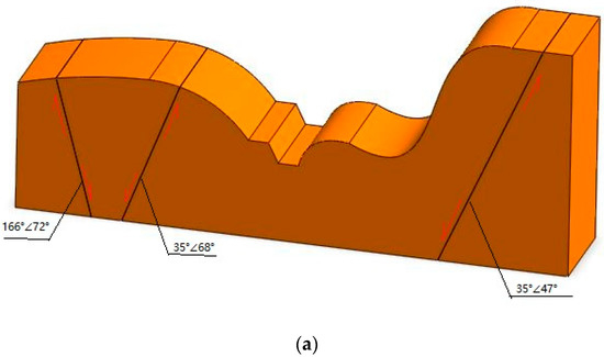
Figure 11.
Investigation area fault model. (a) Ayihai ditch fault; (b) Longcai gorge normal fault; (c) normal fault on the north bank of Longyangxia dam; (d) fault on the west side of Tulin; (e) Duolong ditch fault; (f) positions of small faults.
4.1.3. Determination of In-Situ Stress Based on Focal Mechanism Solution
According to the inversion results of earthquake focal mechanism in the previous section, the maximum horizontal principal stress (8 km–33 km) is generally NE, and in the northwest of Gonghe County, the maximum principal stress is along NE and NNE; in the southwest of the county, the orientation of maximum principal stress is in NE by E; from northeast to southeast of the county, the orientation of the maximum principal stress changes little. The maximum principal stress direction is near NE. As a result of the medium continuity of Kriging interpolation, the regression results show that the maximum principal stress in the region is gradually changing. In the southwest of the geothermal field, the gradient changes greatly due to the large number of seismic sources and different fault properties. In Gonghe Basin, the orientation of maximum principal stress is NE 0°–80° and the dip angle of maximum principal stress is 44°–90°. In the geothermal field, the orientation of maximum principal stress is NE 37° and the dip angle of maximum principal stress is 35.9°.
4.1.4. Comprehensive Analysis of In-Situ Stress Field Direction
According to the focal mechanism solution, inversion analysis of small faults and joint fracture statistics, we can get the variation of in-situ stress direction with depth as shown in the Table 3.
Table 3.
Comprehensive inversion results of principal stress direction.
Comprehensive analysis shows that the orientation of maximum principal stress in the shallow layer is between NE 55° and 72°, and the dip angle is 45°–81.5°. At the depth of more than 5 km, the orientation of maximum principal stress is NE 37° and the dip angle of maximum principal stress is 35.9°.
4.2. Inversion of In-Situ Stress
There are mainly two kinds of inversion methods for rock mass in-situ stress field: (1) Inversion of in-situ stress field by considering topography, geology, and lithology according to measured values of some control points in the engineering area; (2) calculating the magnitude and orientation of in-situ stress based on the measured displacement data and referring to the mechanical properties of local rocks [29]. For most rock mass engineering, it is an important and effective way to carry out inversion, regression, and simulation by theoretical or numerical analysis based on field measured data, considering the characteristics of topography and geology, so as to infer the value of in-situ stress and give the initial mode of in-situ stress field [7]. No matter what kind of analysis method is adopted, the initial stress field of rock mass analyzed should conform to the actual distribution law of in-situ stress field, that is to say, it should conform to the following two principles: (1) The calculated initial in-situ stress field should be basically consistent with the measured value at the measured point; (2) the calculated initial stress field should be in accordance with the influence of topography, geomorphology, and geological conditions on the situation of in-situ stress field, that is to ensure the field coincidence [30].
4.2.1. Principle of Inversion Model
The in-situ stress value of deep well site is determined by numerical simulation software, and the model is elastic model. The stress–strain of the material is in accordance with the generalized Hooke’s law. The three-dimensional stress–strain relationship is as follows:
where, , , are the triaxial strain, ,, are the triaxial stress, ,, are the shear stress, ,, are the shear strain. E is elastic modulus, G is shear modulus and is Poisson’s ratio.
The relationship between the three-dimensional stress and the principal stress is as follows:
where is the main stress, and its coordinate axis coincides with the three principal stress directions.
Through the above transformation, we established the relationship between three principal stresses and deformation.
According to the distribution of in-situ stress, stress boundary conditions are applied on the surface of the model. The stress applied to the model element is assumed by each node.
where is the stress acting on the surface of the model element, A is the surface area of the model element, F is the node force, n is the number of nodes, and i is the node number.
Since the initial displacement boundary conditions are not set in the model, the model will produce a large displacement in the process of equilibrium. After the satisfactory in-situ stress field is obtained, the static equilibrium state of rock mass under the initial in-situ stress field can be simulated by clearing all the node velocity fields and displacement fields of the model. Then, displacement boundary conditions can be added for subsequent calculation.
4.2.2. Inversion of In-Situ Stress
Firstly, we investigated the in-situ stress of some shallow sites. According to the survey results, in the depth of 30–60 m, except that the main stress value of No.1 measuring point is in the southwest direction, the stress values of the other four measuring points are in the northeast direction, about 55 degrees. Except point 1, the dip angle is below 25 degrees. The dip angle of No.1 point is 32 degrees, and the data are abnormal, which may be because it is just near the fault zone. To sum up, the shallow in-situ stress is mainly distributed in the NE direction within 60 m, N in 60–80 m, and NW in 80–100 m. According to the measured data, Figure 12 is obtained through regression analysis. According to the regression analysis curve, R2 is 0.5493, the correlation is medium, so regression analysis can be carried out.
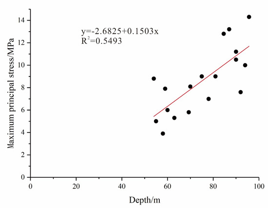
Figure 12.
Stress regression analysis of surface survey points.
Then we use the 3D geological model to inverse the deep in-situ stress. Firstly, the contour lines of the area with 1 m precision were obtained from large-scale high-definition three-dimensional topographic map, and the three-dimensional terrain surface in the region was established. Then, according to the drilling data, the 3D geological model is established. According to the core conditions, the stratigraphic distribution is established, and a total of 9 strata are established. The mechanical parameters and types of rock strata are shown in the Table 4.
Table 4.
Rock types and rock mechanics parameters.
Since there is only one well in this area, the established strata are all horizontal except surface layer. The model is set to 3000 m × 3000 m × 4000 m, and the analysis area is large enough to eliminate the abnormal stress field caused by the boundary conditions imposed on the central target well area, and improve the reliability of the results. Different from the traditional cube model, the physical geological model considers the influence of surface topography, mountain unloading and other factors on in-situ stress, in order to make the results closer to the reality. The in-situ stress in the shallow part was inverted by regression analysis, so that the calculated stress field and the measured stress field can achieve the optimal fitting. There is no in-situ stress data measured in the deep, so the boundary method is used for inversion in combination with the regional overall in-situ stress and the in-situ stress direction of the small area. The drilling and production direction is set as Z direction, and the horizontal plane is XY plane to use the boundary stress method to impose boundary conditions. The establishment model is shown in Figure 13.
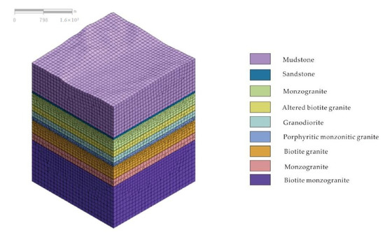
Figure 13.
3D geological model.
Based on the previous orientation distribution of in-situ stress and the boundary conditions obtained from the in-situ stress, there are regularly changes of the orientation of maximum principal stress with the change of depth. The positive direction of Y axis and X axis corresponds to the geographic north direction and east direction. According to the stress direction change curve, we add boundary load conditions as follows [12]:
- (1)
- The load boundary conditions were applied to the two sides of X-axis and Y-axis to simulate the horizontal tectonic forces. With the increase of depth, the ratio of uniform load in X-axis to Y-axis changes from tan 49.82° to tan 54.39°. In the process of simulation, the ratio should be adjusted to be consistent with the actual situation.
- (2)
- To simulate the gravity, we apply the gravity acceleration g in the Z-axis direction of the 3D geological model.
The software simulation results are shown in Figure 14, Figure 15 and Figure 16. According to the analysis results, the principal stress values are increasing from shallow to deep, and the overall change is uniform. Based on the analysis of the software calculation results, the variation trend of ground stress is shown in Figure 17. At the depth of 3500 m, the maximum principal stress reaches 82 MPa and the stress gradient is about 0.0234 MPa/m; the minimum principal stress reaches 45 MPa, and the stress gradient is about 0.0141 MPa/m; the intermediate principal stress reaches 70 MPa, and the stress gradient is about 0.02 MPa/m.
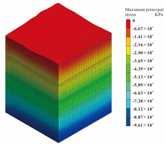
Figure 14.
Distribution of maximum principal stress.
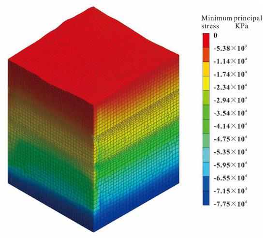
Figure 15.
Distribution of minimum principal stress.
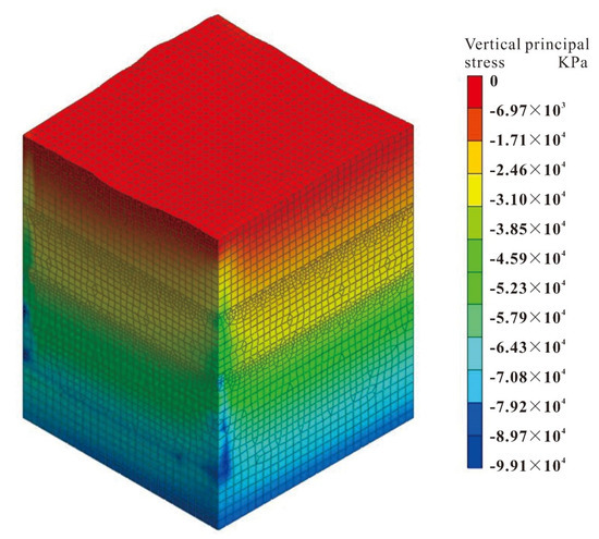
Figure 16.
Distribution of vertical principal stress.
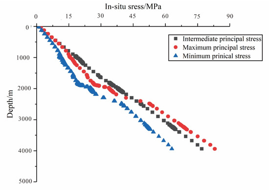
Figure 17.
Variation of in-situ stress with depth.
5. Induced Earthquake Risk Assessment Based on ANN
ANN model is used to evaluate the risk of induced earthquake in the Qiabuqia geothermal field. Each ANN model represents an actual earthquake. Although more seismic data information can provide more accurate prediction results, thousands of seismic data collection and analysis datasets are not realistic. Therefore, we selected 98 representative sets of data, including 13 earthquakes with Ms ≥ 5.0 and 78 earthquakes with 5.0 > Ms ≥ 3.0 in the history of geothermal field area, and 7 induced earthquakes occurred in typical geothermal development sites in the world. Based on these 98 sets of data, an ANN model is used to predict the maximum magnitude and focal mechanism of the earthquake induced in the Qiabuqia geothermal field.
Artificial neural network establishes a certain model from the perspective of information processing, and forms different networks according to different connection modes [31,32]. The ANN model mainly considers the topological structure of network connections, the characteristics of neurons and learning rules. According to the different algorithms in topological structure, ANN can be divided into many different types. At present, the algorithms used for earthquake prediction include BP algorithm, genetic algorithm, probability algorithm and so on. BP neural network algorithm was used in this paper. BP neural network has the ability of arbitrary complex pattern classification and excellent multi-dimensional function mapping, including two processes of signal forward propagation and error back-propagation. In structure, BP network has an input layer, hidden layer, and output layer. In essence, BP algorithm takes the square of network error as the objective function and uses gradient descent method to calculate the minimum value of objective function.
The neurons of three levels are responsible for the input, transformation, and output of information and numerical control, respectively. Figure 18 shows a neural network system with 18 neurons in three layers. Its working principle is as follows:
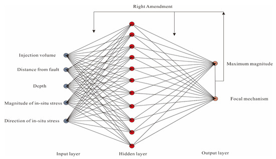
Figure 18.
Schematic diagram of neural network model.
Let the input vector be:
where M is the number of learning pattern pairs and N is the number of neurons in the input layer.
Akn = (a1n, a2n, …, ann) (k = 1, 2, 3, …, M; n = 1, 2, 3, …, N)
The expected output vector Yk = (y1, y2, …, yp), which is the number of neurons in the output layer. The input of each unit cell in the middle layer is calculated as follows:
where Wij is the connection weight between input layer and middle layer; θj is the threshold value of middle layer neurons; p is the number of middle layer neurons.
In order to ensure the nonlinear characteristics of the model and the output of the middle layer neurons, Si is used as the independent variable of Sigmoid function. The Sigmoid function takes:
where f(x) is called the excitation function. The activation value of neurons in the middle layer was as follows:
Information flows from the input layer to the output layer. Given the input information, the corresponding output results are obtained.
where Lt is the input value of each unit cell in the output layer; Ct is the output value of the network.
We can see that there is a three-layer network which can reflect the mapping of any continuous function with any precision, but if we want to construct this mapping, we need to train the neural network model.
The calculation accuracy and speed of the BP neural network model depend on the parameters of its structure layer, so the first task of modeling is to determine the parameters of the mechanism layer reasonably. In this training model, the amount of hidden layers is set to 1 and the amount of hidden layer nodes is set to 11. The maximum training times are 5000, the learning rate is 0.001, and the training accuracy is 0.00001.
The input parameters include injection volume, distance from fault, depth, magnitude, and orientation of in-situ stress, and output parameters are magnitude and focal mechanism, as shown in Table 5.
Table 5.
Seismic parameters for simulation training.
There are only 20 sets of seismic parameters in Table 5, including 13 earthquakes with Ms ≥ 5.0 and 7 induced earthquakes occurred in typical geothermal sites. All 98 sets of data are substituted into the ANN model for simulation training, and the data are preprocessed before the parameters are input, that is, the injection volume, the distance from the fault, the depth, the magnitude of in-situ stress, and the orientation of in-situ stress are represented by logarithm, which can improve the accuracy of the model. The effect of model training is shown in Figure 19.
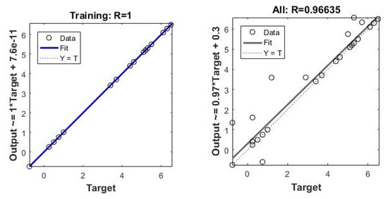
Figure 19.
Fitting diagram of training data.
It can be seen from the figure that the training data and all the data fit well, with R of 1 and 0.96635, respectively (the closer the R value to 1, the better the fitting situation). Gradient is the function of gradient descent method, and Validation Checks is the error test to prevent excessive learning in the process of model training. Before training, a step number will be set for validation set. For example, the default value is 6 epochs. Then the system will judge whether the error does not decrease after six consecutive tests. If it does not decrease or even increase, it indicates that the training error of training set is no longer reduced and has no better effect. Then, it is unnecessary to train again and stop training.
According to the trained neural network model, the induced earthquakes by hydraulic fracturing in the Qiabuqia geothermal field are evaluated and predicted, and the results are shown in Figure 20.
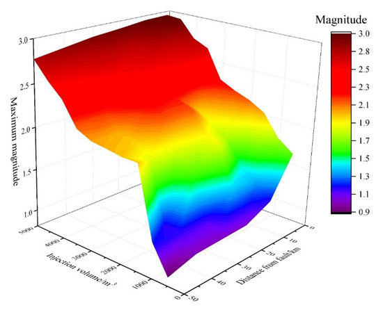
Figure 20.
Surface plot of maximum magnitude with variable injection volume and distance from fault.
In this neural network model, there are five variables and two output values. In the Qiabuqia geothermal field, the drilling depth is 3500 m, so the value of in-situ stress is 82 MPa and the orientation of in-situ stress is NE 37°. The maximum earthquake magnitude caused by hydraulic fracturing is predicted by changing the volume of injected water and the distance from fault. The magnitude increases with the increase of injection volume, as shown in Figure 20. When the injection volume reaches 5000 m3, the maximum magnitude is close to magnitude 3. At the same time, with the decrease of the distance from the fault, the magnitude of seismicity also increases slowly, but not obviously. When the injection volume is small, the phenomenon that the magnitude increases with the decrease of distance is difficult to detect. However, when the injection volume is large, such as more than 3500 m3, this phenomenon becomes obvious gradually. In addition, most of the focal mechanism of induced earthquakes are reverse faults, accounting for 70%, of which 25% are sinistral reverse and 45% are dextral reverse, as shown in Figure 21. Normal faults account for only 30%, including 18.3% sinistral normal and 11.7% dextral normal.
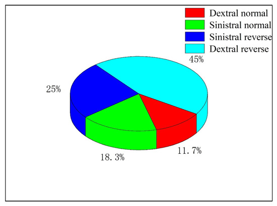
Figure 21.
Proportion of different focal mechanisms.
Figure 22 shows the magnitude equipotential line of induced earthquake with water injection volume of 5000 m3 obtained from neural network model. We can draw the result from the figure that the maximum magnitude occurred near the well site, with a maximum magnitude of 2.96. The magnitude of the earthquake decreases gradually from the center to the periphery in the vicinity of the well site, and is affected by the fault tectonism. With the decrease of the distance from the fault, the magnitude increases to a certain extent.
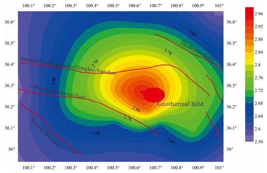
Figure 22.
Equipotential lines for predicting induced earthquake magnitude.
Compared with the actual situation, the prediction result should be larger. There are two reasons. Firstly, only five factors are considered in the ANN model, but there are still many parameters affecting induced earthquakes in actual production. These five parameters have the most important influence on the induced earthquake, so we choose these five parameters as the input layer of the ANN model. However, the influence of other parameters, such as injection pressure and injection fluid properties, cannot be completely ignored. Secondly, the training data we selected are natural earthquake data with Ms >3 and large induced earthquake data that have occurred, which will definitely make the result larger. Therefore, our forecast result will be larger than the actual situation, but still has reference significance.
6. Conclusions
In this paper, we first summarize and analyze the regional tectonic evolution based on the survey data and regional seismogenic history of the Qiabuqia geothermal field, and obtain the focal mechanism and stress state of earthquakes. Then, according to the field survey data and software simulation, the magnitude and orientation of in-situ stress in the geothermal field are inversed and calculated to obtain the state of in-situ stress. Finally, combined with focal mechanism, in-situ stress state and tectonic situation, the maximum magnitude of hydraulic fracturing induced earthquake is predicted and analyzed by using artificial neural network model. The conclusions are as follows:
- Gonghe Basin is located in the important node area of the Central Orogenic belt where many blocks intersect and transform. Its seismicity is relatively frequent. There are 97 earthquakes with Ms ≥ 3.0 and 13 earthquakes with Ms ≥ 5.0 since the 1950s near the geothermal field, which are basically distributed along the main fault zones, and most of the focal mechanisms are dextral reverse faults.
- Comprehensive analysis of joint fracture statistics, structure analysis of small fault and focal mechanism solution, the orientation of maximum principal stress in the shallow layer is between NE 55° and 72°, and at the depth of more than 5 km, the direction of maximum principal stress is NE 37°.
- According to the field investigation and the software simulation inversion results, the principal stress values are increasing from shallow to deep, and the overall change is uniform. The maximum principal stress gradient is about 0.0234 MPa/m, reaching 82 MPa at 3500 m depth. The minimum principal stress gradient is about 0.0141 MPa/m, reaching 45 MPa at 3500 m depth. The intermediate principal stress gradient is about 0.02 MPa/m, reaching 70 MPa at 3500 m depth.
- The trained ANN model is used to predict and evaluate the earthquake induced by hydraulic fracturing in the Qiabuqia geothermal field. The results show that the magnitude increases with the increase of injection volume and with the decrease of the distance from the fault. The maximum magnitude is close to magnitude 3.
Author Contributions
Conceptualization, K.S.; Data curation, K.S.; Funding acquisition, Y.Z. (Yanjun Zhang); Investigation, Y.Z. (Yanhao Zheng); Methodology, K.S.; Project administration, Y.Z. (Yanjun Zhang); Resources, Y.Z. (Yanjun Zhang); Software, Y.Z. (Yanhao Zheng), L.L. and H.D.; Validation, H.D.; Writing—Original draft, K.S.; Writing—Review & Editing, Y.Z. (Yanjun Zhang). All authors have read and agreed to the published version of the manuscript.
Funding
This study was supported by the New Energy Program of Jilin Province (NO. SXGJSF2017-5), the National Key R&D Program of China (NO.2018YFB1501803), and the National Natural Science Foundation of China (NO. 41772238).
Conflicts of Interest
The authors declare no conflict of interest.
References
- Sanyal, S.K.; Butler, S.J. An analysis of power generation prospects from enhanced geothermal system. In Proceedings of the World Geothermal Congress, Antalya, Turkey, 24–29 April 2005. [Google Scholar]
- Zeng, Y.C.; Wu, N.Y.; Su, Z. Numerical simulation of electricity generation potential from fractured granite reservoir through a single horizontal well at Yangbajing geothermal field. Energy 2014, 65, 472–487. [Google Scholar] [CrossRef]
- Stephens, J.C.; Jiusto, S. Assessing innovation in emerging energy technologies:socio-technical dynamics of carbon capture and storage (CCS) and enhanced geothermal systems (EGS) in the USA. Energy Policy 2010, 38, 2020–2031. [Google Scholar] [CrossRef]
- Genter, A.; Evans, K.; Cuenot, N.; Fritsch, D.; Sanjuan, B. Contribution of the exploration of deep crystalline fractured reservoir of soultz to the knowledge of enhanced geothermal systems (EGS). Comptes Rendus Geosci. 2010, 342, 502–516. [Google Scholar] [CrossRef]
- Majer, E.L.; Baria, R.; Stark, M.; Oates, S.; Bommer, J.; Smith, B.; Asanuma, H. Induced seismicity associated with Enhanced Geothermal Systems. Geothermics 2007, 36, 185–222. [Google Scholar] [CrossRef]
- Martínez-Garzón, P.; Bohnhoff, M.; Kwiatek, G.; Dresen, G. Stress tensor changes related to fluid injection at The Geysers geothermal field, California. Geophys. Res. Lett. 2013, 40, 2596–2601. [Google Scholar] [CrossRef]
- Boyd, O.S.; Dreger, D.S.; Gritto, R.; Garcia, J. Analysis of seismic moment tensors and in situ stress during Enhanced Geothermal System development at The Geysers geothermal field, California. Geophys. J. Int. 2018, 215, 1483–1500. [Google Scholar] [CrossRef]
- Baisch, S.; Weidler, R.; Voros, R.; Wyborn, D.; de Graaf, L. Induced seismicity during the stimulation of a geothermal HFR reservoir in the Cooper Basin, Australia. Bull. Seism. Soc. Am. 2006, 96, 2242–2256. [Google Scholar] [CrossRef]
- Kwiatek, G.; Bulut, F.; Bohnhoff, M.; Dresen, G. High-resolution analysis of seismicity induced at Berlín geothermal field, El Salvador. Geothermics 2014, 52, 98–111. [Google Scholar] [CrossRef]
- Baisch, S.; Vörös, R.; Rothert, E.; Stang, H.; Jung, R.; Schellschmidt, R. A numerical model for fluid injection induced seismicity at Soultz-sous-Forêts. Int. J. Rock Mech. Min. Sci. 2010, 47, 405–413. [Google Scholar] [CrossRef]
- Kraft, T.; Deichmann, N. High-precision relocation and focal mechanism of the injection-induced seismicity at the Basel Egs. Geothermics 2014, 52, 59–73. [Google Scholar] [CrossRef]
- Lei, Z.; Zhang, Y.; Yu, Z.; Hu, Z.; Li, L.; Zhang, S.; Fu, L.; Zhou, L.; Xie, Y. Exploratory research into the enhanced geothermal system power generation project: The Qiabuqia geothermal field, Northwest China. Renew. Energy 2019, 139, 52–70. [Google Scholar] [CrossRef]
- Lei, Z.; Zhang, Y.; Zhang, S.; Fu, L.; Hu, Z.; Yu, Z.; Li, L.; Zhou, J. Electricity generation from a three-horizontal-well enhanced geothermal system in the Qiabuqia geothermal field, China: Slickwater fracturing treatments for different reservoir scenarios. Renew. Energy 2020, 145, 65–83. [Google Scholar] [CrossRef]
- Pijush, S.; Dookie, K. Applicability of artificial intelligence to reservoir induced earthquakes. Acta Geophys. 2014, 62, 608–619. [Google Scholar]
- Esen, H.; Inalli, M.; Sengur, A.; Esen, M. Performance prediction of a groundcoupled heat pump system using artificial neural networks. Expert Syst. Appl. 2008, 35, 1940–1948. [Google Scholar] [CrossRef]
- Esen, H.; Inalli, M. Modelling of a vertical ground coupled heat pump system by using artificial neural networks. Expert Syst. Appl. 2009, 36, 10229–10238. [Google Scholar] [CrossRef]
- Gang, W.J.; Wang, J.B. Predictive ANN models of ground heat exchanger for the control. Appl. Energy 2013, 112, 1146–1153. [Google Scholar] [CrossRef]
- Zhou, L.; Zhang, Y.; Hu, Z.; Yu, Z.; Luo, Y.; Lei, Y.; Lei, H.; Lei, Z.; Ma, Y. Analysis of influencing factors of the production performance of an enhanced geothermal system (EGS) with numerical simulation and artificial neural network (ANN). Energy Build. 2019, 200, 31–46. [Google Scholar] [CrossRef]
- Zamani, A.; Sorbi, M.R.; Safavi, A.A. Application of neural network and ANFIS model for earthquake occurrence in Iran. Earth Sci. Inform. 2013, 6, 71–85. [Google Scholar] [CrossRef]
- Zhang, S.Q.; Yan, W.D.; Li, D.P.; Jia, X.; Zhang, S.; Li, S.; Mu, J.Q. Characteristics of geothermal geology of the Qiabuqia HDR in Gonghe basin, Qinghai Province. Geol. China 2018, 45, 1087–1102. [Google Scholar]
- Meng, Q. Analysis of heavy minerals in sediments of xining-guide Basin in northeastern margin of the Tibet plateau in Cenozoic era and its tectonic evolution. Acta Sedimentol. Sin. 2013, 31, 139–148. [Google Scholar]
- Zhang, C.; Gong, J.; Zou, X.; Dong, G.; Li, X.; Dong, Z. Estimates of soil movement in a study area in Gonghe Basin, north-east of Qinghai-Tibet Plateau. J. Arid Environ. 2003, 53, 285–295. [Google Scholar] [CrossRef]
- Kagan, Y.Y.; Jackson, D.D. Likelihood analysis of earthquake focal mechanism distributions. Geophys. J. Int. 2015, 201, 1409–1415. [Google Scholar] [CrossRef]
- Mukuhira, Y.; Fuse, K.; Naoi, M.; Fehler, M.C.; Moriya, H.; Ito, T.; Asanuma, H.; Häring, M.O. Hybrid focal mechanism determination: Constraining focal mechanisms of injection induced seismicity using in situ stress data. Geophys. J. Int. 2018, 215, 1427–1441. [Google Scholar] [CrossRef]
- Kuang, W.; Zoback, M.; Zhang, J. Estimating geomechanical parameters from microseismic plane focal mechanisms recorded during multistage hydraulic fracturing. Geophysics 2017, 82, KS1–KS11. [Google Scholar] [CrossRef]
- Li, H.; Yao, Z.X. Microseismic focal mechanism inversion in frequency domain based on general dislocation point model. Chin. J. Geophys. 2018, 61, 905–916. [Google Scholar] [CrossRef]
- Convertito, V.; Herrero, A. Influence of Focal Mechanism in Probabilistic Seismic Hazard Analysis. Bull. Seismol. Soc. Am. 2004, 94, 2124–2136. [Google Scholar] [CrossRef]
- Karatela, E.; Taheri, A.; Xu, C.; Stevenson, G. Study on effect of in-situ stress ratio and discontinuities orientation on borehole stability in heavily fractured rocks using discrete element method. J. Pet. Sci. Eng. 2016, 139, 94–103. [Google Scholar] [CrossRef]
- Sasaki, S.; Kaieda, H. Determination of stress state from focal mechanisms of microseismic events induced during hydraulic injection at the Hijiori hot dry rock site. Pure Appl. Geophys. 2002, 159, 489–516. [Google Scholar] [CrossRef]
- Boyle, K.; Zoback, M. The Stress State of the Northwest Geysers, California Geothermal Field, and Implications for Fault-Controlled Fluid Flow. Bull. Seismol. Soc. Am. 2014, 104, 2303–2312. [Google Scholar] [CrossRef]
- Arcaklioglu, E.; Erisen, A.; Yilmaz, R. Artificial neural network analysis of heat pumps using refrigerant mixtures. Energy Convers. Manag. 2004, 45, 1917–1929. [Google Scholar] [CrossRef]
- Kumar, R.; Aggarwal, R.K.; Sharma, J.D. Energy analysis of a building using artificial neural network: A review. Energy Build 2013, 65, 352–358. [Google Scholar] [CrossRef]


Publisher’s Note: MDPI stays neutral with regard to jurisdictional claims in published maps and institutional affiliations. |
© 2020 by the authors. Licensee MDPI, Basel, Switzerland. This article is an open access article distributed under the terms and conditions of the Creative Commons Attribution (CC BY) license (http://creativecommons.org/licenses/by/4.0/).