Derivation and Uncertainty Quantification of a Data-Driven Subcooled Boiling Model

Abstract

Subcooled flow boiling occurs in many industrial applications where enormous heat transfer is needed. Boiling is a complex physical process that involves phase change, two-phase flow, and interactions between heated surfaces and fluids. In general, boiling heat transfer is usually predicted by empirical or semiempirical models, which are horizontal to uncertainty. In this work, a data-driven method based on artificial neural networks has been implemented to study the heat transfer behavior of a subcooled boiling model. The proposed method considers the near local flow behavior to predict wall temperature and void fraction of a subcooled minichannel. The input of the network consists of pressure gradients, momentum convection, energy convection, turbulent viscosity, liquid and gas velocities, and surface information. The outputs of the models are based on the quantities of interest in a boiling system wall temperature and void fraction. To train the network, high-fidelity simulations based on the Eulerian two-fluid approach are carried out for varying heat flux and inlet velocity in the minichannel. Two classes of the deep learning model have been investigated for this work. The first one focuses on predicting the deterministic value of the quantities of interest. The second one focuses on predicting the uncertainty present in the deep learning model while estimating the quantities of interest. Deep ensemble and Monte Carlo Dropout methods are close representatives of maximum likelihood and Bayesian inference approach respectively, and they are used to derive the uncertainty present in the model. The results of this study prove that the models used here are capable of predicting the quantities of interest accurately and are capable of estimating the uncertainty present. The models are capable of accurately reproducing the physics on unseen data and show the degree of uncertainty when there is a shift of physics in the boiling regime.

1. Introduction

Engineering applications with high heat flux generally involve boiling heat transfer. The high heat transfer coefficient reached by boiling flows makes boiling heat transfer relevant for research where thermal performance enhancement is needed. Although boiling heat transfer can improve the cooling performance of a system, the underlying physics are not fully understood yet. Therefore, it remains a major challenge to model the boiling heat transfer behavior for a boiling system.

Among other methods, the two-fluid model-based computational fluid dynamics (CFD) has shown a good capability of dealing with boiling flow heat transfer problems. In such an approach, information of the interface between vapor and liquid is taken as an average using closure equations, resulting in lower computational power requirements. Two-fluid models represent a promising solution to develop high fidelity representations, where all the concerned fields can be predicted with good accuracy. One of the most known two-fluid approach based CFD models to simulate boiling flows is the Rensselaer Polytechnic Institute (RPI) model, proposed by Kurul et al. [1]. The RPI model proposes to decompose the total applied heat flux on the wall on three components to take into account the evaporation, forced convection, and the quenching. Many authors adopted this approach to model the boiling flows in different geometries and for multiple operating conditions [2,3,4,5]. When comparing their results to the available experimental data, fair agreements were obtained only for few fields, while bad estimations were obtained for many others. The fields of interest here are the vapor void fraction, the different phases velocities and temperatures, and the heated surface temperature. These failed estimations are related principally to the use of several closure models representing phenomenons occurring at different length scales, as the momentum and mass transfer at the interface, bubbles interaction in the bulk flow, and more importantly mechanical and thermal interactions on the heated surface, leading to nucleation, evaporation, bubble growth and departure, etc. These closure equations are developed based on empirical or mechanistic treatments. The first is based on experimental data that are valid only for reduced ranges of operating conditions, and when they are extrapolated, accurate results are no longer guaranteed. Mechanistic treatments are based on several assumptions that generally neglect the complicated interactions between bubbles, interactions between the heated surface and fluids, and they represent a hard linking between the occurring phenomenons time and space scales.

The field of fluid dynamics is closely linked to massive amounts of data from experiments and high-fidelity simulations. Big data in fluid mechanics has become a reality [6] due to advancements in experimental techniques and high-performance computing (HPC). Machine learning (ML) algorithms are rapidly advancing within the fluid mechanics domain, and ML algorithms can be an additional tool for shaping, speeding up, and understanding complex problems that are yet to be fully solved. They provide a flexible framework that can be tailored for a particular problem, such as reduced-order modeling (ROM), optimization, turbulence closure modeling, heat transfer, or experimental data processing. For example, proper orthogonal decomposition (POD) has been successfully implemented to obtain a low-dimensional set of ordinary differential equations, from the Navier–Stokes equation, via Galerkin projection [7,8]. POD technique has been used to investigate the flow structures in the near-wall region based on measurements and information from the upper buffer layer at different Reynolds number for a turbulent channel [9]. However, it has been reported that the POD method lacks in handling huge amount of data when the size of the computational domain increases [10]. On the other hand, artificial neural networks (ANN) are capable of handling huge data size and nonlinear problems of near-wall turbulent flow [11]. ANNs have been used to learn from large eddy simulation (LES) channel flow data, and it is capable of identifying and reproducing highly nonlinear behavior of the turbulent flows [12]. In the last few years, there have been multiple studies related to the use of ANNs for estimating the subgrid-scale in turbulence modeling [13,14,15]. Among other neural networks, convolution neural networks (CNNs) have been widely used for image processing due to their unique feature of capturing the spatial structure of input data [16]. This feature is an advantage when dealing with fluid mechanics problems since CNN allows us to capture spatial and temporal information of the flows. Multiple CNN structure [17] has been proposed to predict the lift coefficient of airfoils with different shapes at different Mach numbers, Reynolds number, and angle of attack. A combination of CNN with multi-layer perceptron (MLP) [18] has been used to generate a time-dependent turbulent inflow generator for a fully developed turbulent channel flow. The data used for that work have been obtained from direct numerical simulation (DNS), and the model was able to predict the turbulent flow long enough to accumulate turbulent statistics.

Machine learning techniques are rapidly making inroads within heat transfer and multiphase problems too. These ML methods consist of a series of data-driven algorithms that can detect a pattern in large datasets and build predictive models. They are specially designed to deal with large, high-dimensional datasets, and have the potential to transform, quantify, and address the uncertainties of the model. ANN-based on the back-propagation model has been used to predict convective heat transfer coefficients in a tube with good accuracy [19]. Experimental data from impingement jet with varying nozzle diameter and Reynolds number have been used to build an ANN model. This model was then used to predict the heat transfer (Nusselt number) with an error bellow 4.5% [20]. More recently, researchers have used ANN for modeling boiling flow heat transfer of pure fluids [21]. Neural networks have been used to fit DNS data to develop closure model relation for the average two-fluid equations of vertical bubble channel [22]. The model trained on DNS data was then used for different initial velocities and void fraction, to predict the main aspects of DNS results. Different ML algorithms [23] have been examined to study pool boiling heat transfer coefficient of aluminum water-based nanofluids, and their result showed that the MLP network gave the best result. In the past, CNNs model has been used even as an image processing technique for two-phase bubbly flow, and it has been shown that they can determine the overlapping of bubbles: blurred and nonspherical [24].

Although there is research related to boiling heat transfer and machine learning algorithms, according to the authors’ knowledge all the above-mentioned models focus on deterministic ANN models. When working with a reduced order model or black-box model such as deep learning models for physical applications, it becomes of prime importance to know the model confidence and capability. If these models are to be used for a new set of operating conditions, the first thing to consider is how reliable this model is and how accurate the predicted value is. Therefore, it is crucial to know the uncertainty present in the predictions made.

The aforementioned ML techniques applied to heat transfer and fluid mechanics are mostly deterministic approaches that lack in providing predictive uncertainty information. At the same time, deterministic ANN models tend to produce overconfident predictions, which may lead to unpredictable situations when used in real-life industrial applications. Therefore, it is essential to quantify the uncertainty present in the model for any practical applications. Uncertainty models provide the user with the confidence level, and they allow them to make better decisions based on engineering judgment.

In Bayesian learning, a priori distribution is defined upon the parameters of a NNs, then given the training data, the posterior distribution over the parameter is computed, which is used to estimate the predictive uncertainty [25]. The fundamental concern in Bayesian learning while analyzing data or making decisions is to be able to tell whether the model is certain about its output. Bayesian-based models offer a mathematically grounded framework to reason about model uncertainty, but the computational cost rapidly increases as the data size increases. Due to computational constraints in performing exact Bayesian inference, several approximation methods have been proposed such as; Markov chain Monte Carlo (MCMC) [26] method, variational Bayesian methods [27,28], Laplace approximation [29], probabilistic backpropagation (PBP) [30]. The nature of predictive quality using Bayesian NNs depends on correct priori distribution and degree of approximation of Bayesian inference due to high computational cost [31]. However, Bayesian models are harder to implement, they make it harder to define the correct priori properties, and they are computationally slower compared to traditional neural networks. Another approach to quantify the uncertainty of an ANN model is the Deep Ensemble method [32], which is inspired by the bootstrap technique [33]. In this method, it is assumed that the data has a parametrized distribution where the parameters depend on the input. Finding these parameters is the aim of the training process, i.e., the prediction network will not output a single value but instead will output the distributional parameters of the given input.

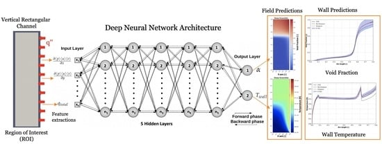
It is worth mentioning that this work presents one of the first attempts to implement deep learning techniques and quantify the model uncertainty of a data-driven subcooled boiling model. In this work, three data-driven models using deep learning techniques have been investigated to study the heat transfer behavior of a subcooled boiling in a minichannel with varying inflow velocity and heat fluxes. The first model focuses on the prediction of the deterministic value of the void fraction and wall temperature of the minichannel which are quantities of interest (QoIs). The second and third model focuses on probabilistic deep learning techniques to derive the uncertainty in the models when predicting the QoIs. The two methods used are Deep Ensemble, which is representative of the Maximum Likelihood approach, and Monte Carlo Dropout, which is representative of Bayesian inference. These two models are capable of capturing the nonlinear behavior that exists in the subcooled boiling data and is capable of reproducing the physics of unseen data for both interpolation and extrapolation datasets.

2. Methodology

2.1. CFD Modeling

There are two methods when it comes to modeling of boiling flows. The first approach is Volume of Fluid (VoF), which employs interface tracking to give a better understanding of the bubbles nucleation and ebullition cycle [34,35]. However, an extremely large grid needs to be employed to perform this kind of simulation and it is computationally expensive. On the other hand, the Eulerian approach is based on averaging the conservation equations with selected interfacial terms. This makes it more appropriate for this work, since the goal is to model boiling in a full channel scale. Therefore, in this work CFD simulations were carried out based on an Eulerian two-fluid approach for modeling the subcooled nucleate boiling flows. The conservation equations for each phase, i.e., liquid and vapor phases, are solved numerically based on a Finite-Volume discretization implemented in the open-source platform OpenFOAM. The presented number of model details, correlations, and assumptions have been evaluated and used in [5].

The mass conservation equation for each phase, liquid continuous phase or vapor dispersed phase, can be written as:

$$\frac{\partial {\alpha }_k{\rho }_k}{\partial t}+\nabla ·\left({\alpha }_k{\rho }_k{\mathbf{U}}_k\right)={\Gamma }_{ki}-{\Gamma }_{ik}$$

(1)

where the subscript k denotes the phase, $\alpha$ is the void fraction, $\rho$ is the phase density, U is the phase velocity and $\Gamma$ is the mass transfer rate per unit volume that denotes evaporation or condensation, calculated based on the boiling equations that will be presented later.

For each phase k, the following momentum conservation is solved based on the following equation:

$$\frac{\partial {\alpha }_k{\rho }_k{\mathbf{U}}_k}{\partial t}+\nabla ·\left({\alpha }_k{\rho }_k{\mathbf{U}}_k{\mathbf{U}}_k\right)=-{\alpha }_k\nabla p+{\mathbf{R}}_k+{\mathbf{M}}_k+{\alpha }_k{\rho }_k\mathbf{g}+\left({\Gamma }_{ki}{\mathbf{U}}_i-{\Gamma }_{ki}{\mathbf{U}}_k\right)$$

(2)

where $\nabla p$ is the pressure gradient, R is the combined turbulent and laminar stress term, calculated based on the Reynolds analogy, g is the gravitational acceleration, and M is the interfacial momentum transfer, accounted for the drag forces calculated based on Schiller and Naumann [36] drag coefficient, the virtual mass forces calculated based on a constant coefficient equal to 0.5, and the turbulent dispersion forces calculated based on the model of de Bertodano [37].

The energy transport equation is written in terms of specific enthalpy h for each phase k as follows:

$$\frac{\partial {\alpha }_k{\rho }_k{h}_k}{\partial t}+\nabla ·\left({\alpha }_k{\rho }_k{\mathbf{U}}_k{h}_k\right)={\alpha }_k\frac{Dp}{Dt}+\nabla \left({\alpha }_k{D}_{t,k}^{eff}\nabla h_k\right)+{\Gamma }_{ki}{h}_i-{\Gamma }_{ik}{h}_k+Q_{wall,k}$$

(3)

where $D_{t,k}^{eff}$ is the effective thermal diffusivity, and $Q_{wall,k}$ is the product of the applied heat flux on the wall with the contact area with the wall per unit volume.

In order to account for the turbulent behavior of the dispersed phase flow, the $k-\epsilon$ turbulence model was used for the vapor phase. However, the bubbles-induced turbulence needs to be accounted also in the turbulent flow behavior of the continuous phase. Hence, the Lahey $k-\epsilon$ [38] turbulence model is adopted for the liquid phase.

In order to calculate the mass transfer rates, a boiling model is needed. The approach implemented follows the very well known RPI model after Kurul and Podowski [1], where the total applied heat flux $q_w^{″}$ on the wall is divided into three components, evaporation heat flux $q_{w,e}^{″}$, forced convection heat flux $q_{w,c}^{″}$, and quenching heat flux $q_{w,q}^{″}$. The total applied heat flux can be written as follows:

$$q_w^{″}=q_{w,e}^{″}+q_{w,c}^{″}+q_{w,q}^{″}$$

(4)

To be able to calculate each heat flux contribution, the closure boiling equation applied at the heated surface needs to be specified, as the active nucleation site density $N_a$, the bubble departure diameter $d_{dep}$, and the bubble departure frequency $f_{dep}$. The mathematical expressions of each heat flux contribution can be found in [1,39].

The Active Nucleation Site Density (ANSD) that represents the cavities from where bubbles are nucleated, is calculated based on the correlation of Benjamin and Balakrishnan [40] given by:

$$N_a=218{\mathrm{Pr}}_l^{1.63}\Delta T_{sup}^3{\gamma }^{-1}{\theta }^{-0.4}$$

(5)

where Pr${}_l$ is the liquid Prandtl number, $\Delta T_{sup}$ is the wall superheat, $\gamma$ is a coefficient taking into account the liquid and heated surface thermophysical properties and $\theta$ is a coefficient taking into account the heated surface roughness and the system pressure.

The Bubble Departure Diameter (BDD) is a parameter that represents the nucleating bubble critical diameter, beyond which the bubble leaves its nucleation site. In this work, this parameter is calculated based on the semiempirical model of Ünal [41], given as follows:

$$d_{dep}=\frac{2.42{10}^{-5}{p}^{0.709}a}{\sqrt{b\varphi }}$$

(6)

where a and b are the model coefficients, taking into account the working fluid and the heated surface thermophysical properties, and $\varphi$ is a parameter controlled by the local flow velocity.

The last closure equation for the boiling model is the Bubble Departure Frequency (BDF), representing the number of bubbles leaving a nucleation site per unit time. It is calculated according to the mechanistic model of Brooks and Hibiki [42] as:

$$f_{dep}=\frac{C_{fd}{\mathrm{Ja}}_w^{0.82}{N}_T^{-1.46}{{\rho }^{*}}^{-0.93}{\mathrm{Pr}}_{sat}^{2.36}}{d_{dep}^2}$$

(7)

where $C_{fd}$ is the model coefficient depending on the size of the channel where boiling occurs, $N_T$ is a dimensionless temperature, ${\rho }^{*}$ is a dimensionless density ratio, Ja${}_w$ is a modified Jacob number, and Pr${}_{sat}$ is the liquid Prandtl number evaluated at the corresponding saturation temperature.

Now, the mass transfer rates can be calculated as follows:

$$\begin{array}{c}\hfill {\Gamma }_{evap}=\frac{A_{w,b,e}^f}{6}{\rho }_v{d}_{dep}{f}_{dep}\end{array}$$

(8)

$$\begin{array}{c}\hfill {\Gamma }_{cond}=\frac{h_c\left(T_{sat}\left(p\right)-T_l\right)}{h_{lg}}{A}_s\end{array}$$

(9)

where $A_{w,b,e}^f$ is an area fraction of the heated surface not affected by bubbles, $h_c$ is a condensation heat transfer coefficient calculated based on the correlation of Ranz et al. [43], and $h_{lg}$ is the latent heat of vaporization.

In the previously presented equation system, the selected models and correlations are developed and used in [5]. This numerical model is also used in this work to provide complete datasets of results needed for the present investigation.

2.2. CFD Simulation Data

Data used in this work are obtained from 2D CFD simulations based on the Eulerian two-fluid approach. The computational domain is illustrated in Figure 1. It consists of a narrow rectangular upward channel (0.003 × 0.4 m), heated from one side by a constant uniform heat flux. Water as working fluid is flowing upward the channel at atmospheric pressure. At the channel inlet, the liquid velocity and temperature are set. At the channel walls, a nonslip boundary condition is set for both phases, liquid, and vapor. Since the channel is heated only from one side, the boiling closure equations, i.e., active nucleation site density, bubble departure diameter, and frequency models, are applied on this particular wall. The thermophysical properties of the liquid are calculated based on the inlet temperature, while the vapor and heated surface thermophysical properties are evaluated at the saturation temperature. However, the current numerical code allows the calculation of the local saturation temperature based on the computed local pressure. Multiple heat fluxes and inlet velocities were used to conduct the simulations. In total, 102 simulations have been performed for inlet velocity ranging from 0.05 ms${}^{-1}$ to 0.2 ms${}^{-1}$ and heat flux ranging from 1000 Wm${}^{-2}$ to 40,000 Wm${}^{-2}$. The developed CFD model was validated in a previous work presented in [5] based on experimental result of [44,45]. The heated surface temperature measurements were compared against the CFD predictions and good agreements were obtained.

2.3. CFD Validation

To validate the CFD results used in this work predictions of the onset of nucleate boiling are compared to the experimental measurements of Kromer et al. [45], as shown in

Table 1. CFD validation for the void fraction with the experimental data provided by [45].

Heat Flux ${\mathit{q}}^{″}$	${\mathit{Z}}_{\mathbf{ONB}}$ [Kromer et al. [45]	${\mathit{Z}}_{\mathbf{ONB},\mathbf{CFD}}$	Error
Wm${}^{-2}$	(mm)	(mm)	%
30,000	$188.9\pm 0.5$	172	9
20,000	$192.3\pm 0.5$	240	25

. The simulated heated surface temperature, is compared to the measurements of Al-Maeeni [44] and is presented in Figure 2. The experimental results of Kromer et al. [45] and Al-Maeeni [44] were based on upward flow boiling in a narrow aluminum rectangular channel (3 × 10 × 400 mm). They used water as working fluid medium, and the channel was heated from one side with a constant heat flux. Kromer et al. [45] used a mass flux of 58.1 kgm${}^{-2}$s${}^{-1}$ with two different heat fluxes, $q^{″}$ = 20,000 Wm${}^{-2}$ and $q^{″}$ = 30,000 Wm${}^{-2}$, whereas Al-Maeeni used a mass flux of 134.2 kgm${}^{-2}$s${}^{-1}$ with a heat flux of $q^{″}$ = 50,000 Wm${}^{-2}$. It is to be noted that both the experiments were conducted under the same inlet subcooling $\Delta T_{sub,in}$ = 10 K. From Table 1 it can be seen that a reasonable agreement is achieved for the onset nucleate boiling for both tested heat fluxes, with a maximum error less than 25%. However, a much better agreement is achieved for the heated surface temperature, with a maximum error of 3% between the measurements and the CFD predictions as shown in Figure 2. The predictions associated with the boiling closure equations used in this work are the ANSD model of Benjamin and Balakrishanan [40], the BDD model of Ünal [41], and the BDF model of Brooks and Hibiki [42] (Current model). The CFD results are further compared with the predictions associated with the boiling closure equations given by Benjamin and Balakrishnan [40] for the ANSD, the BDD of Tolubinski and Kostanchuk [46], and the BDF of Cole [47] (Previous model). The comparison of the experiments and the models predictions are shown in Figure 2. It can be noted from the plot that the current model used in this work shows better prediction of the heat surface temperature.

2.4. Data Handling

To train the deep neural network models, data were extracted from the CFD simulations in the region 0 to 0.32 m, which is the selected region of interest (ROI), this is done to avoid the influence of boundary near the outlet. The ROI for extracting the data is shown in Figure 1. The number of cells present in the ROI are 321 × 26 resulting in 8346 data points for each case. The domain axes (x and y) are further converted into nondimensional numbers by diving with the maximum length value of the minichannel. This is done so that the model is not constrained to learn based on the height of the channel and applicable for other channel lengths. Out of the 102 simulated cases, 96 cases are used for training and validating the models, while the remaining 6 cases are used for further analyzing the model performance. These 96 cases are split into 80% (Training Dataset) for training the model and 20% (Validation Dataset) for validation. The validation and test dataset are used for evaluating the models. The validation dataset is predominately used to describe the evaluation of models when tuning hyperparameters and data preparation, and the test dataset is predominately used to describe the evaluation of a final model when comparing it to other final models. Hence, the remaining 6 test cases are used to provide an unbiased evaluation of the final model fit on the training dataset.

The selected feature input signals obtained from CFD simulations are shown in

Table 2. Input features used for training the network.

Input Features	Feature Expressions
Pressure gradient	$\frac{\partial \langle p\rangle }{\partial x}$
	$\frac{\partial \langle p\rangle }{\partial y}$
Momentum convection	$\frac{\partial \langle p\rangle \langle u\rangle \langle u\rangle }{\partial x}$
	$\frac{\partial \langle p\rangle \langle u\rangle \langle v\rangle }{\partial x}$
	$\frac{\partial \langle p\rangle \langle u\rangle \langle v\rangle }{\partial y}$
	$\frac{\partial \langle p\rangle \langle v\rangle \langle v\rangle }{\partial y}$
Energy convection	$\frac{\partial \langle p\rangle \langle T\rangle \langle u\rangle }{\partial x}$
	$\frac{\partial \langle p\rangle \langle T\rangle \langle v\rangle }{\partial y}$
Total heat flux	$q^{″}$
Inlet velocity	$u_{inlet}$
Inlet pressure	$p_{inlet}$
Temperature inlet	$T_{inlet}$
Ambient pressure	$p_{amb}$
Fluid and gas viscosity	${\mu }_l$${\mu }_g$
Nondimensional x and y axis	$\frac{x}{x_{max}}$, $\frac{y}{y_{max}}$
Nondimensional arc length	$\frac{l}{l_{max}}$

. These inputs are chosen based on their influence on the quantities of interest. The expected outputs (void fraction and wall temperature) from the DNN models are presented in

Table 3. Output features (quantities of interest).

Output Features	Feature Expressions
Wall Temperature	$T_{wall}$
Void Fraction	$\alpha$

. Before feeding the training data into the network, the input and output features are normalized between 0 and 1. This way the ML algorithms can learn better since the scale of data used in this study is very sparse.

2.5. Deep Neural Networks Architectures

Artificial neural networks are computational models that are inspired by the way neurons in brains work. They have the ability to acquire and retain information and generally comprise an input layer, hidden layer, and output layer. These layers are sets of processing units, represented by so-called artificial neurons, interlinked by multiple interconnections, implemented with vectors and matrices of synaptic weights. An ANN with multiple hidden layers is generally known as deep neural network (DNNs) or multi-layer perceptron (MLP).

Two stages are involved while training the MLP network with the back-propagation technique also known as the generalized Delta rule. These stages are illustrated in Figure 3, which shows a MLP with 5 hidden layers, 18 signals on its input layer, $n_1\cdots n_5$ neurons in the hidden layers, and finally 2 output signals. In the first stage, the signals $\{x_1,x_2,\cdots \cdots ,x_n\}$ of the training sets are inserted into the network inputs and are propagated layer-by-layer until the production of the corresponding outputs. Thus, this stage propagates only in the forward direction to obtained the responses (outputs) from the network, hence, it is called the feed-forward phase. The network undergoes series of nonlinear transformation controlled by parameters like weights $\mathbf{W}$ and biases $\mathbf{b}$, followed by a nonlinear activation function ($\mathbf{g}\left(\mathbf{x}\right)$). There is a wide number of activation functions that can be used depending on classification or regression problems. In this work, a nonlinear activation function called rectified linear units (ReLU) is used. The main advantage of ReLU function is that it does not activate all the neurons at the same time. It only activates the neuron if the linear transformation is above zero value and it is computationally efficient. The MLP in Figure 3 can be interpreted as:

$$\begin{array}{ccc}\hfill h_1& =\hfill & \hfill g(W_1^{T}x+b_1)\\ \hfill ..\\ \hfill h_5& =\hfill & \hfill g(W_5^T{h}_4+b_5)\\ \hfill \widehat{y}& =\hfill & \hfill g(W_6^T{h}_5+b_6)\end{array}$$

(10)

$$\begin{array}{ccc}\hfill g\left(x\right)& =\hfill & \hfill \left\{\begin{array}{cc}0\hfill & \mathrm{for}x<0\hfill \\ x\hfill & \mathrm{for}x\ge 0\hfill \end{array}\right.\end{array}$$

(11)

A cost or loss function $\mathcal{L}$ is defined while training the network to measure the error between the predicted value $\widehat{y}$ and the target value y. The type of loss function used while training a neural network is problem specific and depending on whether it is a classification or a regression problem. For this work, mean squared error (MSE) loss is used for computing the loss function. Once the loss is computed, the error gradient concerning weights and biases in all the layers can be computed through a backward phase. The main objective of the backward phase is to estimate the gradient of the loss function for the different weights by using the chain rule of differential calculus. These computed gradients are then used to update the weights and biases of all the hidden layers. In this work, the Adaptive Moment Estimation (Adam) [48] optimization technique is used to update the weights and biases of the network with a learning rate of Lr = $1e^{-4}$. The Adam optimization technique has been chosen due to its capability of handling large datasets, high-dimensional parameters, and sparse gradients. Since these gradients are estimated in the backward direction, starting from the output node, this learning process is referred to as the backward phase.

$$\mathcal{L}=MSE(y,\widehat{y})$$

(12)

While training a deep neural network, it is a common issue that the model becomes overfitted. Overfitting occurs when an algorithm is tailored to a particular dataset and is not generalized to deal with other datasets. To avoid overfitting of the DNN model, a regularization term is generally introduced in the loss function $\mathcal{L}$. The two most common regularization approaches are $\mathcal{L}1$ norm ($Lasso$$Regression$) and $\mathcal{L}2$ norm ($Ridge$$Regression$) and they are expressed:

$$\begin{array}{c}\hfill \mathcal{L}=MSE(y,\widehat{y})+\lambda \sum _{i=1}^N\left|w_i\right|\\ \hfill L_{1}norm\\ \hfill \mathcal{L}=MSE(y,\widehat{y})+\lambda \sum _{i=1}^N{w}_i^2\\ \hfill L_{2}norm\end{array}$$

(13)

where $\lambda$ is a positive hyperparameter that influences the regularization term, with a larger value of $\lambda$ indicating strong regularization.

These regularization terms regularize or shrink the coefficient estimates towards zero, and it has been shown that shrinking the coefficient estimates can significantly reduce the variance [49]. $\mathcal{L}1$ regularization forces the weight parameters to become zero, and $\mathcal{L}2$ regularization forces the weight parameters towards zero but never exactly zero. When regularization term is applied to DNN it results in smaller weight parameters by making some neurons neglectable. This makes the network less complex and avoids overfitting. For this work, $\mathcal{L}2$ norm ($Ridge$$Regression$) regularization is applied in all the hidden layers while training the deep neural network.

2.6. Uncertainty of Deep Learning

Deep learning techniques have attracted considerable attention in fields such as physics, fluid mechanics, and manufacturing [50,51,52]. In these fields estimating model uncertainty is of crucial importance since it is vital to understanding the interpolation and extrapolation ability of the model. Deep learning algorithms are able to learn powerful representations that can map high dimensional data to an array of outputs. These mapping functions are often taken blindly and assumed to be accurate, which may not be always true. Hence, it is of paramount importance to be able to quantify the uncertainty present and justify the behavior of these models. Therefore, in this work, two uncertainty quantification (UQ) models have been investigated to justify the nature of the model and they are described in detail.

2.6.1. Monte Carlo (MC) Dropout method

The deep learning models can be cast as Bayesian models, without changing either the model or the optimization process. This can be done by an approach called dropout during training and prediction, and it has been proven that dropout in ANNs can be interpreted as a Bayesian approximation of a well known probabilistic model, the Gaussian process (GP) [53]. Dropout has been used in many deep learning models as a way to avoid overfitting [54] like regularization technique. Dropout technique in a neural network with some modifications can be used for estimating the uncertainty, as described by Gal et al. [55]. Their method implies that as long as the neural network is trained with few dropout layers, it can be used to estimate the uncertainty of the model during the time of prediction. Unlike traditional Dropout networks, Monte Carlo Dropout (MC Dropout) networks apply dropout both at the training and testing phase.

When a network with input feature $X^{*}$ is trained with dropout, the model is expected to give an output with predictive mean $\mathbb{E}$$\left(y^{*}\right)$ and the predictive variance $Var\left(y^{*}\right)$. To approximate the model as a Gaussian Process, a prior length scale $\mathit{l}$ is defined and captures the belief over the function frequency. A short length-scale $\mathit{l}$ corresponds to high frequency data, and a long length-scale $\mathit{l}$ corresponds to low frequency data. Mathematically the Gaussian process precision $\left(\tau \right)$ is given as:

$$\begin{array}{c}\hfill \tau =\frac{l^{2}p}{2N{\lambda }_w}\end{array}$$

(14)

where p is the probability of the units (artificial neurons) not dropped during the process of training, ${\lambda }_w$ is the weight decay, and N is the size of the dataset. Similarly, dropout is activated during the prediction phase of a new set of data (validation or test data) $x^{*}$, i.e., randomly units are dropped during the prediction phase. The prediction step is repeated several times (T) with different units dropped every time, and results are collected $\left\{\widehat{y}{}_t^{*}\left(x^{*}\right)\right\}$. The empirical estimator of the predictive mean of the approximated posterior and the predictive variance (uncertainty) of the new test data is given by the following equations:

$$\begin{array}{c}\hfill \mathbb{E}\left(y^{*}\right)\approx \frac{1}{T}\sum _{t=1}^T{\widehat{y}}_t^{*}\left(x^{*}\right)\end{array}$$

(15)

$$Var\left(y^{*}\right)\approx {\tau }^{-1}{I}_D+\frac{1}{T}\sum _{t=1}^T{\widehat{y}}_t^{*}{\left(x^{*}\right)}^T{\widehat{y}}_t^{*}\left(x^{*}\right)-\mathbb{E}{\left(y^{*}\right)}^T\mathbb{E}\left(y^{*}\right)$$

(16)

2.6.2. Deep Ensemble

Deep Ensemble [32] is a non-Bayesian method for uncertainty quantification in machine learning models. Deep ensemble learning is a learning paradigm where ensembles of several neural networks show improved generalization capabilities that outperform those of a single network. It has been shown that an ensemble model has good predictive quality and can produce good estimates of uncertainty [32]. In general, while training a neural network for a regression problem, the goal is to minimize the error between the target value $\mathbf{y}$ and the predicted value $\widehat{\mathbf{y}}$ using mean squared error (mse) loss. However, to obtain the uncertainty estimates, the model has to be expressed in the form of a probabilistic model. Hence, this approach assumes that given an input $\mathbf{X}$, the target $\mathbf{y}$ has a normal distribution with a mean and a variance depending on the values of $\mathbf{X}$. This results in modification of the loss function; instead of minimizing the difference of target and predictive value, the goal is to minimize the predictive distribution to the target distribution using the Negative Log-Likelihood (NLL) loss. It is important to use the correct scoring rule while determining the predictive uncertainty of a model, and NLL has been proven to be a proper scoring rule for evaluating predictive uncertainty [56].

$${\mathcal{L}}_{loss}=-log{p}_{\theta }\frac{y_n}{X_n}=\frac{log{\sigma }^2\left(X\right)}{2}+\frac{{(y-{\mu }_{\theta }\left(X\right))}^2}{2{\sigma }^2\left(X\right)}+c$$

(17)

where, ${\mu }_{\theta }\left(X\right)$ and ${\sigma }^2\left(X\right)$ are the predictive mean and the variance, c is a constant. Intuitively, the goal is to minimize the difference between the predictive distribution to the target distribution using the negative log-likelihood loss.

In a Deep Ensemble model, M networks are trained with different random initialization. It is to be noted that as the number of networks increases, the computational cost also increases during the time of training. Therefore, the number of networks to be considered is a trade-off between computational speed and accuracy of the prediction. For this study, 5 networks with random initialization were trained to create the deep ensemble model. Ensemble results are then treated as a uniformly-weighted mixture model, although for simplicity the ensemble prediction is approximated to be a Gaussian distribution whose mean and variance are respectively the mean and variance of the mixture. The mean and variance mixture is given by:

$${\mu }_{*}\left(X\right)=\frac{1}{M}\sum _m{\mu }_{\theta m}\left(X\right)$$

(18)

$${\sigma }_{*}^2\left(X\right)=\frac{1}{M}\sum _m({\sigma }_{\theta m}^2\left(X\right)+{\mu }_{\theta m}^2\left(X\right))-{\mu }_{*}^2\left(X\right)$$

(19)

where ${\mu }_{\theta m}\left(X\right)$ and ${\sigma }_{\theta m}^2\left(X\right)$ are the mean and variance of individual networks, ${\mu }_{*}\left(X\right)$ and ${\sigma }_{*}^2\left(X\right)$ are the mean and variance of the ensemble model respectively. The detailed explanation and benchmark of the deep ensemble model and equations can be found in the research conducted by Lakshminarayanan et al. [32]. To implement the above method in a standard deep learning architecture the following steps were taken: first, a custom loss function with NLL is defined, then another custom layer has been defined to extract the mean and variance as an output of the network.

The summary of all the models investigated in this work is shown in

Table 4. Specification of the models, MSE: Mean Squared Error, NLL: Negative Log-Likelihood, Adam: Adaptive Moment Estimation, Lr: Learning rate, MLP: Multi Layer Perceptron, MC: Monte Carlo.

Models	Input	Hidden	Output	Batch	Uncertainty	Cost/Loss	Optimizer	Lr
	Signals	Layers	Signals	Size	Quantification	Function
MLP	18	5	2	256	No	MSE	Adam	$1e^{-4}$
MC no-Dropout	18	5	2	256	No	MSE	Adam	$1e^{-4}$
MC Dropout	18	5	2	256	Yes	MSE	Adam	$1e^{-4}$
Deep Ensemble	18	5	2	256	Yes	NLL	Adam	$1e^{-4}$

. The Monte Carlo Dropout model has the possibility to predict the quantities of interest with uncertainty (MC Dropout) and without uncertainty (MC no-Dropout) for the same trained model. To avoid overfitting of all the models used in this work, the following measures have been taken into consideration while training the network:

• $L_2$ regularization term is introduced in the loss function.
• Callback functions are defined to save only the best weights of the network, with early stopping of the training if the validation loss does not improve in the next epoch.
• Several batch size were tested and for this study batch size of 256 gave the best results. Batch size in machine learning is the number of training data used in one iteration.
• The best weight saved during the training phase by the callbacks is loaded before the prediction phase.

This way it ensures that the model is not an overfitted model and it uses the best weights of the model while predicting a new unseen case.

3. Results and Discussion

In this work, the open-source deep-learning library Tensorflow 1.14 along with python 3.5 are used to build the architecture of the deep learning models (MLP, MC Dropout, and Deep Ensemble). In total there are 102 CFD datasets for varying heat flux and velocities, out of which 96 cases are split into training data (80%) and validation data (20%). Each case consists of 8346 data points. The remaining 6 cases are purely used for further testing of the model, of which 3 cases for interpolation, and the remaining 3 cases for extrapolation. The model performance is first evaluated using the validation dataset first, then tested on the interpolation dataset, and finally on the extrapolation dataset. The MLP model is a deterministic model whereas the MC Dropout and Deep Ensemble models provide the deterministic values as well as the expected variance of the predicted value. The validation and testing performance of the MLP model is relatively lower when compared to MC Dropout and Deep Ensemble models and the statistic performance can be seen in

Table 5. Performance of the models on validation dataset of the computational domain, VF: Void Fraction, Temp: Temperature.

Case	Models	RMSEP		${\mathit{R}}^2$
Dataset		VF	Temp	VF	Temp
Validation	MLP	0.008	0.152	0.991	0.987
	MC No-Dropout	0.013	0.265	0.995	0.989
	MC Dropout	0.006	0.125	0.9991	0.997
	Deep Ensemble	0.002	0.081	0.9998	0.998

. From the table it can be noted that the DE model shows the best performance. The models used in this study are capable of predicting the void fraction field and temperature field of the minichannel domain. However, the discussion presented in the Section 3.2 and Section 3.3 will be focused on the near-wall region of the minichannel. The near-wall region is of particular interest since there is a sudden shift in physics/behaviors and the motivation was to demonstrate the performance and robustness of the DNN models in this region. For the interested reader, the prediction of the full field flow of the void fraction and temperature in the minichannel is demonstrated in Appendix A through Figure A5–Figure A8.

3.1. Validation Case Studies

The performance of the models is demonstrated using scatter plots, where the models predicted values are plotted against the CFD values for the void fraction as shown in Figure 4. The scatter points in the scatter plots are the full computational domain predicted values using the DNN models. The predicted void fraction using a standard MLP/DNN is plotted against the CFD values, as shown in Figure 4a. The predicted values are mostly concentrated near the x = y line, this line is the true line where the predicted values would perfectly match the CFD results. However, the MLP model has trouble predicting accurately near the void fraction 0 to 0.001, where the nucleation starts in the channel. It can be noted that the MLP model shows nonlinearity around void fraction 0.7 to 0.8, which could be related to change in the flow regime induced by massive generation of bubbles and the MLP model fails to capture the physics in this region. Furthermore, it can be observed that the MLP model shows a void fraction value above unity, which is nonphysical.

The void fraction values predicted using the Monte Carlo Dropout method are presented in Figure 4b. It can be observed that there are two scatter set of results “red”: dropout prediction and “blue”: no-dropout prediction. During the dropout prediction phase, 20% of the neurons in each hidden layer are randomly deactivated every time for 1000 iteration, resulting in 1000 values for each void fraction, the mean value of each void fraction is then plotted. This nature of dropout prediction allows us to quantify the variance of the predicted value, hence it can indicate the degree of uncertainty present in this model. Whereas the blue scatter plot is the predictive value obtained from the model with no-dropout during the prediction phase. It can be seen from the plot that the performance of the dropout prediction outperforms the no-dropout prediction and fits the x = y line better. It can be further observed from the plot that the predicted values are concentrated near the x = y line at low values of void fraction. Then the predicted values start to get sparse as the void fraction value increases and become more sparse around 0.8. This sparsity in fitting the data can be related to change in flow and boiling regime where the underlying physical phenomenon becomes very complex and includes a strong instability in the flow. From the validation dataset, it is evident that the Monte Carlo dropout model captures well when void fraction is low and its performance starts to deteriorate as the void fraction value increases.

The predictive performance of the Deep Ensemble (DE) model on the validation dataset is shown in Figure 4c, where the predicted values are plotted against the CFD value. Unlike the MLP and MC Dropout model, the void fraction value predicted by the DE model does not suffer from sparsity, and the predicted values are concentrated near the x = y line, meaning this model is capable of reproducing the CFD values accurately. It can be further noticed that DE models perform well for void fraction ranging from 0.2 and above, which implies that the DE model seems to capture the physics that exists in these regimes from the data used in training. However, there are some uncaptured nonlinearities present in the model when predicting void fraction values between 0 to 0.05, and this is the region where subcooled boiling starts in the channel. In the region of subcooled boiling, small bubbles start to appear, which changes the dynamics of the flow in the channel. The DE model marginally fails to capture the sudden shift in physics for some of the data points; nevertheless, its performance improves when predicting void fraction for the rest of the subcooled boiling regime. From this, it can be concluded that the DE model captures the main flow features very well for the validation dataset for most of the boiling regimes with some small deviation near the onset of nucleate boiling.

The predicted temperature values are plotted against the CFD values for the computational domain and are shown in Figure 5. The predictive capability of the standard MLP/DNN model is demonstrated in Figure 5a. From the plot, it is evident that the MLP model performs poorly when predicting the temperature. The MLP model shows high nonlinearity between the predicted and CFD values starting from 372 K to 379 K; however, it is still worth mentioning that the maximum relative error percentage is under 0.6%. Figure 5b shows the scatter plot of the CFD value and the MC model predicted values. The scatter plot with blue represents the prediction with no-dropout and the scatter plot with red represents the prediction with dropout activated. It is clear from the plot that the prediction with no-dropout deviates away from the x = y line and it under predicts the temperature. However, when dropout is activated during the prediction phase, the predictions are more concentrated around the x = y line. It can be further noted that the sparsity of the predicted values increases in the range of 373.15 K to 375 K, because for most of the case data subcooled boiling starts around this temperature. The maximum relative error between the CFD and the predicted value for the dropout prediction is below 0.3%. In contrast, the predictive nature of the DE model outperforms the MLP and MC dropout model as shown in Figure 5c. It is evident from the figure that the DE model is capable of perfectly capturing the temperature for all the boiling regimes. After closer inspection, it can be noted that the DE model slightly suffers while predicting the temperature around 374 K to 379 K. The DE model predicts the CFD values very well, with a maximum relative error below 0.05%.

Overall, it can be concluded that the MLP model has lower performance when compared to the MC Dropout and the Deep Ensemble model. Therefore, in the following sections the results obtained from the MLP model for interpolation and extrapolation predictions will not be included in the main part of the discussions. For the interested readers the results are presented in the Appendix A through Figure A1–Figure A4.

3.2. Interpolation Case Studies

To further demonstrate the predictive performance of the models, further unused test datasets are used to independently evaluate the model behavior. Here the interpolation dataset refers to data that were not used during training or the validation as presented in Section 3.1, with heat flux and inlet velocity values within the range of the training data. The statistics of the predictive performance of all the models tested on 3 unseen interpolation cases are given in

Table 6. Performance of the models on interpolation test dataset, VF: Void Fraction, Temp: Temperature. Interpolation * is the tested data presented in the results.

Case	U	${\mathit{q}}^{″}$	Models	RMSEP		${\mathit{R}}^2$
Datasets	ms${}^{-1}$	Wm${}^{-2}$		VF	Temp	VF	Temp
Interpolation *	0.05	14,000	MLP	0.0050	0.162	0.998	0.953
			MC No-Dropout	0.0310	0.417	0.992	0.695
			MC Dropout	0.0030	0.146	0.999	0.962
			Deep Ensemble	0.0005	0.011	0.999	0.999
Interpolation	0.075	20,000	MLP	0.006	0.154	0.996	0.972
			MC No-Dropout	0.024	0.381	0.994	0.832
			MC Dropout	0.004	0.117	0.999	0.984
			Deep Ensemble	0.001	0.009	0.999	0.999
Interpolation	0.15	21,000	MLP	0.0040	0.052	0.992	0.998
			MC No-Dropout	0.0040	0.185	0.993	0.976
			MC Dropout	0.0030	0.037	0.997	0.999
			Deep Ensemble	0.0006	0.006	0.999	0.999

. It can be seen that the DE model has the lowest RMSEP for the predicted void fraction and wall temperature.

The results presented here are for a heat flux of $q^{″}$ = 14,000 Wm${}^{-2}$ and an inlet velocity of u = 0.05 ms${}^{-1}$. The scatter plots of the predicted void fraction by MC model and DE model are plotted against the CFD value and are shown in Figure 6a,b. From Figure 6a, it is evident that the prediction with dropout activated outperforms the prediction with no dropout. In the case of no-dropout prediction, the MC model suffers as the void fraction increases and starts to deviate from the x = y line. The deviation in the predicted value is due to change in the boiling regime, and the no-dropout prediction fails to capture the change of regime. However, when dropout is activated in the MC model the predicted values fit well to the x = y line. Still, there is a slight predictive performance deterioration near the zero value, where the bubble starts to form in the channel. Aside from that, the dropout model is capable of accurately replicating the CFD values. The DE model has superior prediction performance for void fraction as shown in Figure 6b.

The predicted wall temperature values against the CFD values are shown in the Figure 6c,d. The values predicted using the MC model are presented in the Figure 6c, and it can be noticed that there is poor performance for wall temperatures above 375 K. The MC Dropout model slightly suffers to predict accurately the trend of wall temperature. Nonetheless, it is worth mentioning that the regression plot shows a maximum relative error between the CFD value and the MC dropout predicted value below 0.2%. The wall temperature values predicted by the DE model are shown in Figure 6d. From the scatter plot it can be inferred that the predicted values fit well with the x = y line. Unlike the MC dropout model, the DE model is capable of predicting all the boiling flow regimes with excellent accuracy.

The predicted profile of the void fraction and the uncertainty of the predicted values by the DNN probabilistic models along the nondimensional arc length are presented in Figure 7. Nondimensional arc length refers to the height of the minichannel near the wall. The prediction obtained from MC Dropout is illustrated in Figure 7a. It can be observed that the prediction with no-dropout under performs starting from the void fraction of 0.55 to 0.6, while the prediction with dropout keeps up with the CFD trend. The uncertainty of the predictive value is presented in terms of standard deviation $\sigma$; the filled region represents ±3 $\sigma$. The filled region indicates the confidence level of the model when used for predicting unseen cases. It can be further noted that the model confidence level varies along the nondimensional arc length depending on the regime of subcooled boiling. It can be seen that there is a sudden increase in uncertainty just before a void fraction value of 0.1. This is due to nucleation occurring near the wall, causing phase change. The uncertainty of the model expands as the void fraction approaches unity; this could be related to very complex phenomena and strong instability in the flow. Whereas in Figure 7b, it can be seen that the variation in uncertainty is considerably lower compared to that of MC Dropout predicted value, which makes the DE model more robust. The DE model shows very little uncertainty near the onset of nucleate boiling and almost zero uncertainty until the void fraction approaches unity. From this, it can be noted that the DE model is capable of accurately reproducing the physical phenomena on an unseen interpolation case study.

The predicted wall temperature profile and the uncertainty present along the arc length near the wall of the minichannel is shown in Figure 8. The comparison of CFD vs no-dropout, and dropout temperature profile is presented in Figure 8a. It can be noted that the value predicted with no-dropout is far away from the CFD value, especially after the critical heat flux point (377.2 K). On the other hand, the value predicted with dropout is in close range to that of CFD value, but it slightly over predicts, i.e., between an arc length of 0.6 to 0.8. The filled region in the plot presents the confidence level of the model and it is represented as ±3 $\sigma$. It is evident from the plot that the uncertainty of the MC model is fairly constant until the nondimensional arc length of 0.6. Then the uncertainty of the model starts to peak as the arc length increases. To sum up, the MC model is capable of indicating where the model performance is likely to be good and deteriorate depending on the subcooled flow boiling regimes. In contrast, the ±3 $\sigma$ for the DE model is relatively small compared to the MC dropout model and it is shown in Figure 8b. The DE model predicted wall temperature over lapse with the CFD wall temperature, which signifies that the model is capable of closely replicating the CFD data. It can be further noted that the DE model accurately predicts the temperature profile near with low uncertainty.

From the results seen above and from Table 6 for both the models tested on the interpolation dataset, it can be concluded that the DE model has a better performance in predicting wall temperature and void fraction. The DE model also showed less uncertainty variation compared to the MC Dropout model. Therefore, the DE model is more robust for this specific problem and datatype. For the interested readers, the correlation and sensitivity that exist between the wall temperature and void fraction are shown in Appendix A through Figure A9. A detailed flow field prediction of void fraction and temperature of the minichannel by the MLP model and the DE model is shown in the Appendix A through Figure A5 and Figure A6.

3.3. Extrapolation Case Studies

As expected, the models performed well for the interpolation data. This leads naturally to the next step or evaluating the models’ prediction performance on an extrapolation dataset. To evaluate model capability, tests are performed on three cases where heat flux values are not within the range of the original training datasets. The statistical performance of all the DNN models when tested on 3 unseen extrapolation cases are listed in

Table 7. Performance of the models tested on extrapolation dataset, VF: Void Fraction, Temp: Temperature. Extreme Extrapolation * is the tested data presented in the results.

Case	U	${\mathit{q}}^{″}$	Models	RMSEP		${\mathit{R}}^2$
Datasets	ms${}^{-1}$	Wm${}^{-2}$		VF	Temp	VF	Temp
Extrapolation	0.125	25,000	MLP	0.0040	0.082	0.998	0.993
			MC No-Dropout	0.0130	0.285	0.987	0.917
			MC Dropout	0.0020	0.055	0.999	0.996
			Deep Ensemble	0.0004	0.010	0.999	0.999
Extrapolation	0.1	30,000	MLP	0.0110	0.180	0.990	0.986
			MC No-Dropout	0.0250	0.581	0.994	0.866
			MC Dropout	0.0090	0.101	0.999	0.995
			Deep Ensemble	0.0006	0.015	0.999	0.999
Extreme Extrapolation *	0.2	40,000	MLP	0.016	0.298	0.989	0.962
			MC No-Dropout	0.021	0.577	0.982	0.861
			MC Dropout	0.006	0.092	0.998	0.996
			Deep Ensemble	0.005	0.064	0.999	0.998

. Once again, it can be noted from the table that the DE model outperforms other models.

The results presented here for the extreme extrapolation dataset have a heat flux of $q^{″}$ = 40,000 Wm${}^{-2}$ and an inlet velocity of 0.2 ms${}^{-1}$. It is worth mentioning that the highest heat flux value present in the training data was $q^{″}$ = 29,000 W/m${}^2$, which implies that there is a huge gap in heat flux between the training data and the tested extrapolation dataset. The main motivation was to see if the data-driven models are capable of capturing the physics from the data used for training. Interestingly, it will be shown that these models are capable of accurately replicating the quantities of interest.

The scatter plot in Figure 9 shows the predicted void fraction and the wall temperature by the DNN probabilistic models against the CFD values. From Figure 9a, it can be noted that the prediction with no-dropout deviates from the x = y line, especially above a void fraction value of 0.2. It is clear from the regression plot that this model under predicts. Both dropout and no-dropout predictions suffer near the start of the subcooled boiling regime where nucleation is initiated near the wall. However, the dropout model prediction recovers as the void fraction increases. From the scatter plot it can be observed that the MC dropout model prediction slightly suffers when the void fraction value is around 0.2 to 0.3. In contrast, the DE model shows good predictive quality within the start phase of subcooled boiling, as seen in Figure 9b. Although the model has no problem to accurately predict the beginning of bubble formation, there is mild under prediction for the void fraction range of 0.15 to 0.25, where the number of bubbles generated grows in the channel. Nonetheless, the DE model accurately predicts for void fraction above 0.25 and the rest of the boiling regime.

The predicted wall temperature with MC dropout and MC no-dropout is presented in Figure 9c. From the plot, it can be noted that there is poor performance near 374 K for both the predictions. This is maybe related to the variation of the heat transfer coefficient near the inlet of the channel. Similar to the void fraction, the prediction obtained from the no-dropout model also deviates substantially from the x = y line. However, when dropout is activated during the prediction phase, the MC model shows better performance in predicting the wall temperature. From the plot, it can be noted that there is another slight shift near 377 K, which is likely caused by the massive generation of bubbles in the channel. The deflection of the MC dropout prediction from the CFD value has a maximum relative error of 0.2%. On the other hand, the DE model once again shows a good predictive value of the wall temperature and fits well to the x = y line as shown in Figure 9d. From the plot, it can be seen that the DE model slightly over predicts near 374 K, similar to that of the MC Dropout model. For the remaining predicted wall temperature, the DE model coincides with the x = y line.

The comparison of CFD and predicted void fraction along the nondimensional arc length of the minichannel is shown in Figure 10. The uncertainty of the models are shown as the standard deviation ($\sigma$) from the mean value, and the area filled with blue is ±3 $\sigma$. The filled region indicates the model confidence when predicting an unseen dataset, and it also indicates which region is likely to be more uncertain of its predicted values. In this case, the onset nucleate boiling starts around an arc length of 0.2 though the heat flux is high when compared to the interpolation dataset presented above. The delay in the onset of nucleate boiling is because of the difference in velocity of the flow in the channel, for the interpolation data it had an inlet velocity of u = 0.05 ms${}^{-1}$, and for this case, it has an inlet velocity of u = 0.2 ms${}^{-1}$. This indicates that the saturated temperature is reached slower when the inlet velocity is higher, therefore resulting in a delay of the bubble formation in the channel. The void fraction prediction obtained from the MC Dropout model is illustrated in Figure 10a, where the black dash line is the no-dropout prediction and the one in red is the dropout prediction. Comparing both results to the CFD void fraction it is evident that the dropout prediction performs better in following the trend of the CFD values. The uncertainty for this model starts to peak around 0.1 arc length and gradually grows until 0.2 arc length, then there is a sudden jump in the variation of ±3$\sigma$ which is related to change in phase from the liquid to bubble formation. Though the mean value represented by the dropout curve is close to the CFD curve, the ±3$\sigma$ variation for the rest of the subcooled regime remains constant and starts to narrow down as the arc length increases. In conclusion, the MC Dropout model features considerable uncertainty near the nucleate boiling regime, which is maybe due to the continuous generation of bubbles.

In contrast, the DE model has a lower ±3$\sigma$ variation throughout the prediction of void fraction along the nondimensional arc length as shown in Figure 10b. From the plot, it can be seen that there is very little uncertainty present before the start of subcooled boiling, and the model accurately predicts the onset of nucleate boiling. However, as the void fraction increases, the uncertainty of the prediction grows until an arc length of 0.7. This increase in uncertainty is most likely due to the coalescence of tiny bubbles to larger bubbles. Finally, the degree of uncertainty diminishes as the arc length increases and the DE predicted void fraction overlaps with the CFD values. A possible explanation for this behavior of the DE model is that it can identify when there is a change in physics from liquid to vapor or when there are lots of bubbles, and it shows higher uncertainty in such a region.

The predicted wall temperature profile and the uncertainty present in the models are shown in Figure 11. Once again for the MC model, prediction obtained with no-dropout showed lower performance and its value is far away from the CFD values as illustrated by the black dash line in Figure 11a. However, when dropout is activated the predicted values showed good agreement to the CFD results, except near the region of 0.2 arc length where subcooled boiling begins. The degree of uncertainty increases as it approaches the arc length of 0.2, then it approximately remains constant for the rest of the subcooled boiling. The uncertainty trend present in the predicted wall temperature is similar to the one in the predicted void fraction as presented earlier. This implies that there is a correlation between them which is shown in the Appendix A through Figure A10. Interestingly, the uncertainty present in the DE model is relatively smaller compared to the MC Dropout model, as shown in Figure 11b. The predicted wall temperature values are very close and overlay with most of the CFD results, indicating that the model is capable of capturing the physics in the boiling regime from the training data and reproducing on unseen extrapolation dataset. It can be further noted that there is higher uncertainty near the arc length of 0.1, and this is due to unstable forced convective heat transfer between the wall and the fluid in the channel, just before the formation of bubbles.

In conclusion, both models have shown promising results on the extrapolation dataset. The models used are capable of indicating the regions of higher uncertainty while predicting the void fraction and wall temperature. From the results presented above, it can be noted that the DE model has exceptional predictive performance with lower uncertainty and is overall very robust. For the interested readers, the $\sigma$ variation between the wall temperature and void fraction for the extrapolation case are shown in the Appendix A through Figure A10. A detailed flow field prediction of the extrapolation dataset for both void fraction and temperature field is presented in Appendix A through Figure A7 and Figure A8.

4. Conclusions

The objective of this study is twofold: firstly, to measure the accuracy of the predictions of the deep learning models compared to the CFD results and secondly to quantify the confidence level of the predictions. In this work, three supervised deep learning models have been investigated to study the subcooled boiling heat transfer in a vertical minichannel. The first method focuses on the deterministic approach, whereas the second and the third focus on the probabilistic approach to quantify the uncertainty present in the model while predicting the outputs (QoIs). The training data are obtained from CFD simulations based on the Eulerian two-fluid approach, for varying heat fluxes and inlet velocities. In total 102 cases were simulated, out of which 96 cases were used for training (80%) and validation (20%), and the remaining 6 cases were purely used for in-depth evaluation of the model’s interpolation and extrapolation performance.

The models presented in this study showed a good level of accuracy while predicting the void fraction and the wall temperature. However, it has been observed that the deterministic model (standard DNN/ MLP) showed lower performance when predicting the wall temperature and void fraction. It is crucial to be able to justify the predictive nature and the uncertainty present in the model. Therefore, the probabilistic models’ Monte Carlo Dropout and Deep Ensemble methods were investigated to quantify the predictive uncertainty and the confidence level of these DNNs. The output obtained from these probabilistic models is presented in the form of normal distribution rather than a deterministic value, from which the mean value and the variance of the predicted values are calculated.

According to the results presented, it can be stated that both the MC Dropout and Deep Ensemble models were able to capture the physics well from the given training data. Furthermore, they were able to reproduce these physics on unseen interpolation and extrapolation dataset. The predicted mean values, i.e., the void fraction and the wall temperature were very close to the CFD results and both performed better than the deterministic MLP model. In particular, the DE model showed exceptional predictive performance with low uncertainty. It is worth highlighting that both models were able to capture the change in boiling regimes accurately and showed higher uncertainty when there is a sudden shift in physics, for example when the nucleation starts in the minichannel. Moreover, the probabilistic models were able to reproduce the physics with good accuracy on an extreme extrapolation dataset at a heat flux of $q^{″}$ = 40,000 Wm${}^{-2}$, even though the maximum heat flux used while training the models was 29,000 Wm${}^{-2}$. The uncertainty quantification of the models further explains the steep change in void fraction and wall temperature when heat flux and inflow velocity are varied. On average, all the models had a $RMSEP$ error under 5% for the wall temperature and $RMSEP$ error under 2% for the void fraction with coefficient of determination $R^2:0.998$ and $R^2:0.999$, respectively. This shows that the current study can capture the underlying physics that exist in the boiling data and serves as an independent method to predict the QoIs for a new case study.

The only shortcoming of the uncertainty models compared to the standard MLP model is the computational speed, the predictive time of the uncertainty models are one order of magnitude slower compared to the deterministic MLP model. Nevertheless, the predictive time for the uncertainty models are still two orders of magnitude faster than CFD simulation. The predictive speed of uncertainty models is acceptable considering it provides better performance with the confidence levels and is reasonable for the system-level design process. Therefore, the DNN with uncertainty models can be used as a promising tool to speed up the design phase/initial guesses in the thermal management of a subcooled boiling system.

References

1. Kurul, N.; Podowski, M. On the modeling of multidimensional effects in boiling channels. In Proceedings of the 27th National Heat Transfer Conference, Minneapolis, MN, USA, 28–31 July 1991. [Google Scholar]
2. Lai, J.; Farouk, B. Numerical simulation of subcooled boiling and heat transfer in vertical ducts. Int. J. Heat Mass Transf. 1993, 36, 1541–1551. [Google Scholar] [CrossRef]
3. Anglart, H.; Nylund, O. CFD application to prediction of void distribution in two-phase bubbly flows in rod bundles. Nucl. Eng. Des. 1996, 163, 81–98. [Google Scholar] [CrossRef]
4. Končar, B.; Kljenak, I.; Mavko, B. Modelling of local two-phase flow parameters in upward subcooled flow boiling at low pressure. Int. J. Heat Mass Transf. 2004, 47, 1499–1513. [Google Scholar] [CrossRef]
5. Rabhi, A.; Bel Fdhila, R. Evaluation and Analysis of Active Nucleation Site density Models in Boiling. In Proceedings of the Second Pacific Rim Thermal Engineering Conference, Maui, HI, USA, 13–17 December 2019. [Google Scholar]
6. Pollard, A.; Castillo, L.; Danaila, L.; Glauser, M. Whither Turbulence and Big Data in the 21st Century? Springer: Cham, Switzerland, 2016. [Google Scholar] [CrossRef]
7. Aubry, N.; Holmes, P.; Lumley, J.L.; Stone, E. The dynamics of coherent structures in the wall region of a turbulent boundary layer. J. Fluid Mech. 1988, 192, 115–173. [Google Scholar] [CrossRef]
8. Berkooz, G.; Holmes, P.; Lumley, J.L. The proper orthogonal decomposition in the analysis of turbulent flows. Annu. Rev. Fluid Mech. 1993, 25, 539–575. [Google Scholar] [CrossRef]
9. Podvin, B.; Fraigneau, Y.; Jouanguy, J.; Laval, J.P. On self-similarity in the inner wall layer of a turbulent channel flow. J. Fluids Eng. 2010, 132. [Google Scholar] [CrossRef]
10. Chambers, D.; Adrian, R.; Moin, P.; Stewart, D.; Sung, H.J. Karhunen–Loéve expansion of Burgers’ model of turbulence. Phys. Fluids 1988, 31, 2573–2582. [Google Scholar] [CrossRef]
11. Milano, M.; Koumoutsakos, P. Neural network modeling for near wall turbulent flow. J. Comput. Phys. 2002, 182, 1–26. [Google Scholar] [CrossRef] [Green Version]
12. Sarghini, F.; De Felice, G.; Santini, S. Neural networks based subgrid scale modeling in large eddy simulations. Comput. Fluids 2003, 32, 97–108. [Google Scholar] [CrossRef]
13. Ling, J.; Kurzawski, A.; Templeton, J. Reynolds averaged turbulence modelling using deep neural networks with embedded invariance. J. Fluid Mech. 2016, 807, 155–166. [Google Scholar] [CrossRef]
14. Maulik, R.; San, O.; Rasheed, A.; Vedula, P. Subgrid modelling for two-dimensional turbulence using neural networks. J. Fluid Mech. 2019, 858, 122–144. [Google Scholar] [CrossRef] [Green Version]
15. Gamahara, M.; Hattori, Y. Searching for turbulence models by artificial neural network. Phys. Rev. Fluids 2017, 2, 054604. [Google Scholar] [CrossRef]
16. Lcun, Y.; Bottou, L.; Bengio, Y.; Haffner, P. Gradient-based learning applied to document recognition. Proc. IEEE 1998, 86, 2278–2324. [Google Scholar] [CrossRef] [Green Version]
17. Zhang, Y.; Sung, W.J.; Mavris, D.N. Application of convolutional neural network to predict airfoil lift coefficient. In Proceedings of the 2018 AIAA/ASCE/AHS/ASC Structures, Structural Dynamics, and Materials Conference, Kissimmee, FL, USA, 8–12 January 2018; p. 1903. [Google Scholar] [CrossRef] [Green Version]
18. Fukami, K.; Nabae, Y.; Kawai, K.; Fukagata, K. Synthetic turbulent inflow generator using machine learning. Phys. Rev. Fluids 2019, 4, 064603. [Google Scholar] [CrossRef] [Green Version]
19. Jambunathan, K.; Hartle, S.; Ashforth-Frost, S.; Fontama, V. Evaluating convective heat transfer coefficients using neural networks. Int. J. Heat Mass Transf. 1996, 39, 2329–2332. [Google Scholar] [CrossRef]
20. Celik, N.; Kurtbas, I.; Yumusak, N.; Eren, H. Statistical regression and artificial neural network analyses of impinging jet experiments. Heat Mass Transf. 2009, 45, 599–611. [Google Scholar] [CrossRef]
21. Scalabrin, G.; Condosta, M.; Marchi, P. Modeling flow boiling heat transfer of pure fluids through artificial neural networks. Int. J. Therm. Sci. 2006, 45, 643–663. [Google Scholar] [CrossRef]
22. Ma, M.; Lu, J.; Tryggvason, G. Using statistical learning to close two-fluid multiphase flow equations for a simple bubbly system. Phys. Fluids 2015, 27, 092101. [Google Scholar] [CrossRef]
23. Hassanpour, M.; Vaferi, B.; Masoumi, M.E. Estimation of pool boiling heat transfer coefficient of alumina water-based nanofluids by various artificial intelligence (AI) approaches. Appl. Therm. Eng. 2018, 128, 1208–1222. [Google Scholar] [CrossRef]
24. Poletaev, I.; Pervunin, K.; Tokarev, M. Artificial neural network for bubbles pattern recognition on the images. J. Phys. Conf. Ser. 2016, 754, 072002. [Google Scholar] [CrossRef] [Green Version]
25. Bernardo, J.M.; Smith, A.F. Bayesian Theory; John Wiley & Sons: Hoboken, NJ, USA, 2009; Volume 405. [Google Scholar] [CrossRef]
26. Neal, R.M. Bayesian Learning for Neural Networks; Springer Science & Business Media: New York, NY, USA, 1996; Volume 118. [Google Scholar] [CrossRef]
27. Blundell, C.; Cornebise, J.; Kavukcuoglu, K.; Wierstra, D. Weight uncertainty in neural networks. arXiv 2015, arXiv:1505.05424. [Google Scholar]
28. Graves, A. Practical variational inference for neural networks. In Advances in Neural Information Processing Systems; Curran Associates, Inc.: Red Hook, NY, USA, 2011; pp. 2348–2356. [Google Scholar]
29. MacKay, D.J. Bayesian Methods for Adaptive Models. Ph.D. Thesis, California Institute of Technology, Pasadena, CA, USA, 1992. [Google Scholar] [CrossRef]
30. Hernández-Lobato, J.M.; Adams, R. Probabilistic backpropagation for scalable learning of bayesian neural networks. In Proceedings of the International Conference on Machine Learning, Lille, France, 7–9 July 2015; pp. 1861–1869. [Google Scholar] [CrossRef]
31. Rasmussen, C.E.; Quinonero-Candela, J. Healing the relevance vector machine through augmentation. In Proceedings of the 22nd International Conference on Machine Learning, Bonn, Germany, 7–11 August 2005; pp. 689–696. [Google Scholar] [CrossRef] [Green Version]
32. Lakshminarayanan, B.; Pritzel, A.; Blundell, C. Simple and scalable predictive uncertainty estimation using deep ensembles. In Advances in Neural Information Processing Systems; Curran Associates Inc.: Long Beach, CA, USA, 2017; pp. 6402–6413. [Google Scholar] [CrossRef]
33. Breiman, L. Bagging predictors. Mach. Learn. 1996, 24, 123–140. [Google Scholar] [CrossRef] [Green Version]
34. Hirt, C.W.; Nichols, B.D. Volume of fluid (VOF) method for the dynamics of free boundaries. J. Comput. Phys. 1981, 39, 201–225. [Google Scholar] [CrossRef]
35. Wu, J.; Dhir, V.K.; Qian, J. Numerical simulation of subcooled nucleate boiling by coupling level-set method with moving-mesh method. Numer. Heat Transf. Part B Fundam. 2007, 51, 535–563. [Google Scholar] [CrossRef]
36. Schiller, L.; Naumann, Z. VDI Zeitung 1935. Drag Coeff. Correl. 1935, 77, 318–320. [Google Scholar]
37. De Bertodano, M.A.L. Turbulent Bubbly Two-Phase Flow in a Triangular Duct. Ph.D. Thesis, Rensselaer Polytechnic Institute, Troy, NY, USA, 1992. [Google Scholar]
38. Lahey, R.T., Jr. The simulation of multidimensional multiphase flows. Nucl. Eng. Des. 2005, 235, 1043–1060. [Google Scholar] [CrossRef]
39. Del Valle, V.H.; Kenning, D. Subcooled flow boiling at high heat flux. Int. J. Heat Mass Transf. 1985, 28, 1907–1920. [Google Scholar] [CrossRef]
40. Benjamin, R.; Balakrishnan, A. Nucleation site density in pool boiling of saturated pure liquids: Effect of surface microroughness and surface and liquid physical properties. Exp. Therm. Fluid Sci. 1997, 15, 32–42. [Google Scholar] [CrossRef]
41. Ünal, H. Maximum bubble diameter, maximum bubble-growth time and bubble-growth rate during the subcooled nucleate flow boiling of water up to 17.7 MN/m2. Int. J. Heat Mass Transf. 1976, 19, 643–649. [Google Scholar] [CrossRef]
42. Brooks, C.S.; Hibiki, T. Wall nucleation modeling in subcooled boiling flow. Int. J. Heat Mass Transf. 2015, 86, 183–196. [Google Scholar] [CrossRef]
43. Ranz, W.; Marshall, W.R. Evaporation from drops. Chem. Eng. Prog. 1952, 48, 141–146. [Google Scholar]
44. Al-Maeeni, L. Sub-Cooled Nucleate Boiling Flow Cooling Experiment in a Small Rectangular Channel; KTH, School of Engineering Sciences (SCI), Physics; KTH: Stockholm, Sweden, 2015. [Google Scholar]
45. Kromer, H.; Anglart, T.; Al-Maeeni, T.; Bel Fdhila, R. Experimental Investigation of Flow Nucleate Boiling Het Transfer in a Vertical Minichannel. In Proceedings of the First Pacific Rim Thermal Engineering Conference, Hawaii’s Big Island, HI, USA, 13–17 March 2016. PRTEC-14973. [Google Scholar]
46. Tolubinsky, V.I.; Kostanchuk, D.M. Vapour bubbles growth rate and heat transfer intensity at subcooled water boiling. In Proceedings of the International Heat Transfer Conference 4; Begel House Inc.: Danbury, NY, USA, 1970; Volume 23. [Google Scholar]
47. Cole, R. A photographic study of pool boiling in the region of the critical heat flux. AIChE J. 1960, 6, 533–538. [Google Scholar] [CrossRef]
48. Kingma, D.P.; Ba, J. Adam: A method for stochastic optimization. arXiv 2014, arXiv:1412.6980. [Google Scholar]
49. James, G.; Witten, D.; Hastie, T.; Tibshirani, R. An Introduction to Statistical Learning; Springer: New York, NY, USA, 2013; Volume 112. [Google Scholar] [CrossRef]
50. Baldi, P.; Sadowski, P.; Whiteson, D. Searching for exotic particles in high-energy physics with deep learning. Nat. Commun. 2014, 5, 1–9. [Google Scholar] [CrossRef] [PubMed] [Green Version]
51. Parish, E.J.; Duraisamy, K. A paradigm for data-driven predictive modeling using field inversion and machine learning. J. Comput. Phys. 2016, 305, 758–774. [Google Scholar] [CrossRef] [Green Version]
52. Angermueller, C.; Pärnamaa, T.; Parts, L.; Stegle, O. Deep learning for computational biology. Mol. Syst. Biol. 2016, 12, 878. [Google Scholar] [CrossRef]
53. Rasmussen, C.E. Gaussian processes in machine learning. In Summer School on Machine Learning; Springer: Berlin/Heidelberg, Germany, 2003; pp. 63–71. [Google Scholar] [CrossRef] [Green Version]
54. Srivastava, N.; Hinton, G.; Krizhevsky, A.; Sutskever, I.; Salakhutdinov, R. Dropout: A simple way to prevent neural networks from overfitting. J. Mach. Learn. Res. 2014, 15, 1929–1958. [Google Scholar] [CrossRef]
55. Gal, Y.; Ghahramani, Z. Dropout as a bayesian approximation: Representing model uncertainty in deep learning. In Proceedings of the International Conference on Machine Learning (ICML’16), New York, NY, USA, 20–22 June 2016; pp. 1050–1059. [Google Scholar] [CrossRef]
56. Quinonero-Candela, J.; Rasmussen, C.E.; Sinz, F.; Bousquet, O.; Schölkopf, B. Evaluating predictive uncertainty challenge. In Machine Learning Challenges Workshop; Springer: Berlin/Heidelberg, Germany, 2005; pp. 1–27. [Google Scholar] [CrossRef] [Green Version]
Figure 1. CFD simulation domain and selected region of interest for data extraction.
Energies 13 05987 g001
Figure 2. CFD validation for the heated surface temperature with the experimental data provided by [44].
Energies 13 05987 g002
Figure 3. Back propagation deep neural network (DNN) architecture used in this work.
Energies 13 05987 g003
Figure 4. Validation Void Fraction regression chart of the computational domain.
Energies 13 05987 g004
Figure 5. Validation Temperature regression chart of the computational domain.
Energies 13 05987 g005
Figure 6. Regression chart for interpolation dataset using Monte Carlo and Deep Ensemble for void fraction and wall temperature at q″ = 14,000 Wm−2 and u = 0.05 ms−1.
Energies 13 05987 g006
Figure 7. Void Fraction profile along arc length for interpolation dataset using Monte Carlo and Deep Ensemble models at q″ = 14,000 Wm−2 and u = 0.05 ms−1.
Energies 13 05987 g007
Figure 8. Wall temperature profile along arc length for interpolation dataset using Monte Carlo and Deep Ensemble models at q″ = 14,000 Wm−2 and u = 0.05 ms−1.
Energies 13 05987 g008
Figure 9. Regression chart for interpolation dataset using Monte Carlo and Deep Ensemble for void fraction and wall temperature at q″ = 40,000 Wm−2 and u = 0.2 ms−1.
Energies 13 05987 g009
Figure 10. Void Fraction profile along arc length for extreme extrapolation dataset using Monte Carlo and Deep Ensemble models at q″ = 40,000 Wm−2 and u = 0.2 ms−1.
Energies 13 05987 g010
Figure 11. Wall temperature profile along arc length for extreme extrapolation dataset using Monte Carlo and Deep Ensemble models at q″ = 40,000 Wm−2 and u = 0.2 ms−1.
Energies 13 05987 g011