Cost-Effective Outage Management in Smart Grid under Single, Multiple, and Critical Fault Conditions through Teaching–Learning Algorithm †


Abstract
:1. Introduction
- Well-defined control mechanism in each control agent (CA)
- Smart communicating equipment for coordination among CA
- Robust optimal restoration procedure with good scalability index
- Efficient handling of internal and external equipment constraints
2. Problem Formulation
2.1. Objective Function
2.2. Constraints
2.2.1. Radiality Constraint
2.2.2. Power Balance Constraint
2.2.3. Power Flow Constraints
2.2.4. Capacitors’ Capacity Constraints
2.2.5. DGs Capacity Constraints
- Total real and reactive power demand should not exceed the total generation by the DGs
- Individual DGs’ maximum real and reactive power should not be violated.
2.2.6. Frequency Constraint
3. Conception of Active Zones
4. Optimization Strategy
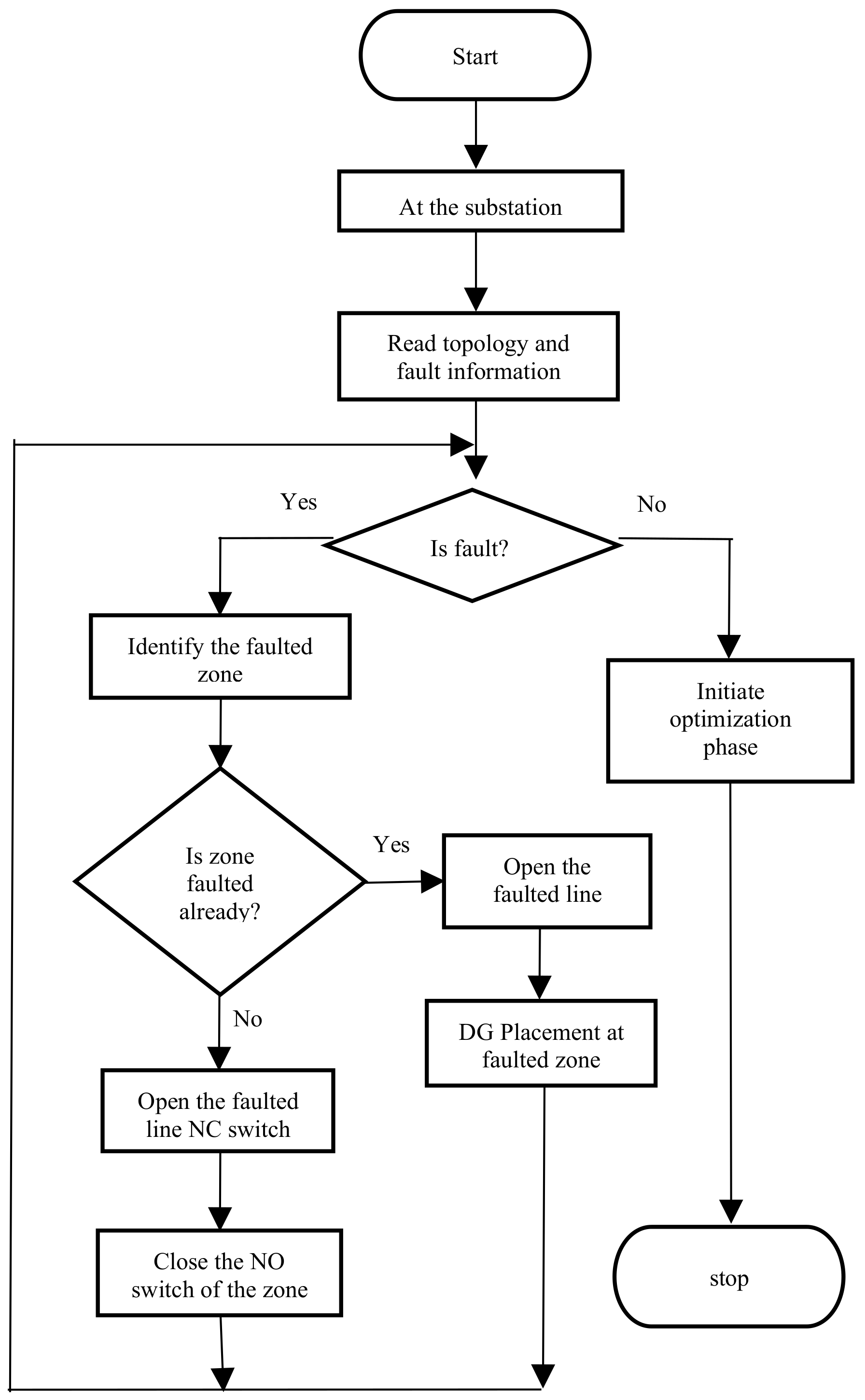
4.1. Restoration Phase
4.2. Optimization Phase
- Unfaulted zone: which is unaffected by a fault
- Faulted zone: which is affected by a fault
- Critical zone: which is affected by multiple faults
- Step 1:
- Identify the critical zone.
- Step 2:
- Restore the unserved loads by DG associated to the zone by the DG agent.
- Step 3:
- Ensure all the constraints are not violated.
- Step 4:
- The line and load data of the distribution system are updated at the load dispatch center.
- Step 5:
- Load dispatch center (LDC) initiates the optimization phase if no further faults are identified in the system.
- Step 6:
- Find the optimal location for DG placement along with reconfiguration and capacitor placement.
- Step 7:
- Relocate the DG for optimal solution.
- Step 8:
- Terminate the process.
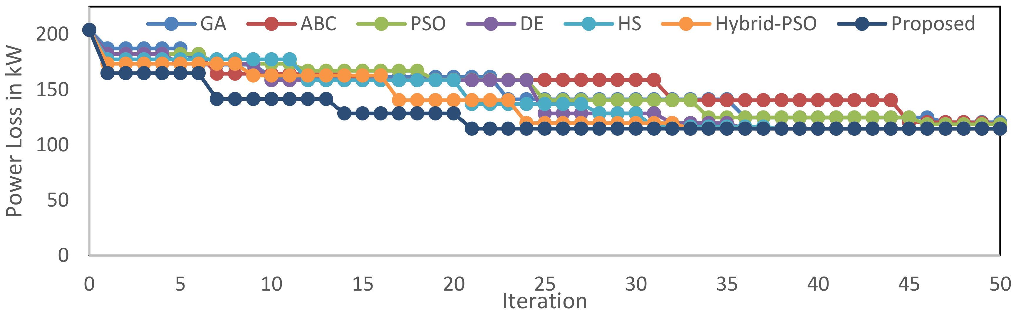
4.3. Teaching Learning Algorithm for the Optimization Process
- Teacher phase: The best learner becomes the teacher in each iteration, where the teacher is the most experienced, knowledgeable, and highly learned person in the community.
- Learner phase: The learners learn the course according to the quality of the teacher and the quality of the learners in the class for each course. The learners get the course input from the teacher and the interaction between the colearners of the class.
- Step 1:
- Initialize total courses offered (C), total learners (L), maximum iteration (MIT), and k = 0.
- Step 2:
- Create the initial population G(C,L).
- Step 3:
- Find the mean of each course, Mj = Meanj(G(C)), j ε C.
- Step 4:
- Identify the best learner that becomes teacher, Tk = Min(f(G)).
- Step 5:
- Create the new population per teacher, Gplus(C,L) = G(C,L) + random() * (Tk − TF*Mj).
- Step 6:
- Produce the best learners’ population, G(C,L) = min(G,Gplus).
- Step 7:
- In interaction between learners, m and n refer to integers (<C) and m ≠ n
- if(f(flearners(m,L)) > f(flearners(n,L)))
- G(m,L) = flearners(m,L) + random()*(flearners(m,L) - flearners(n,L))
- else
- G(m,L) = flearners(m,L) + random()*(flearners(n,L) - flearners(m,L))
- Step 8:
- If k < MIT, update k = k + 1 and go to step 3; else, go to step 9.
- Step 9:
- Print the best solution and terminate the program.
5. Results and Discussions
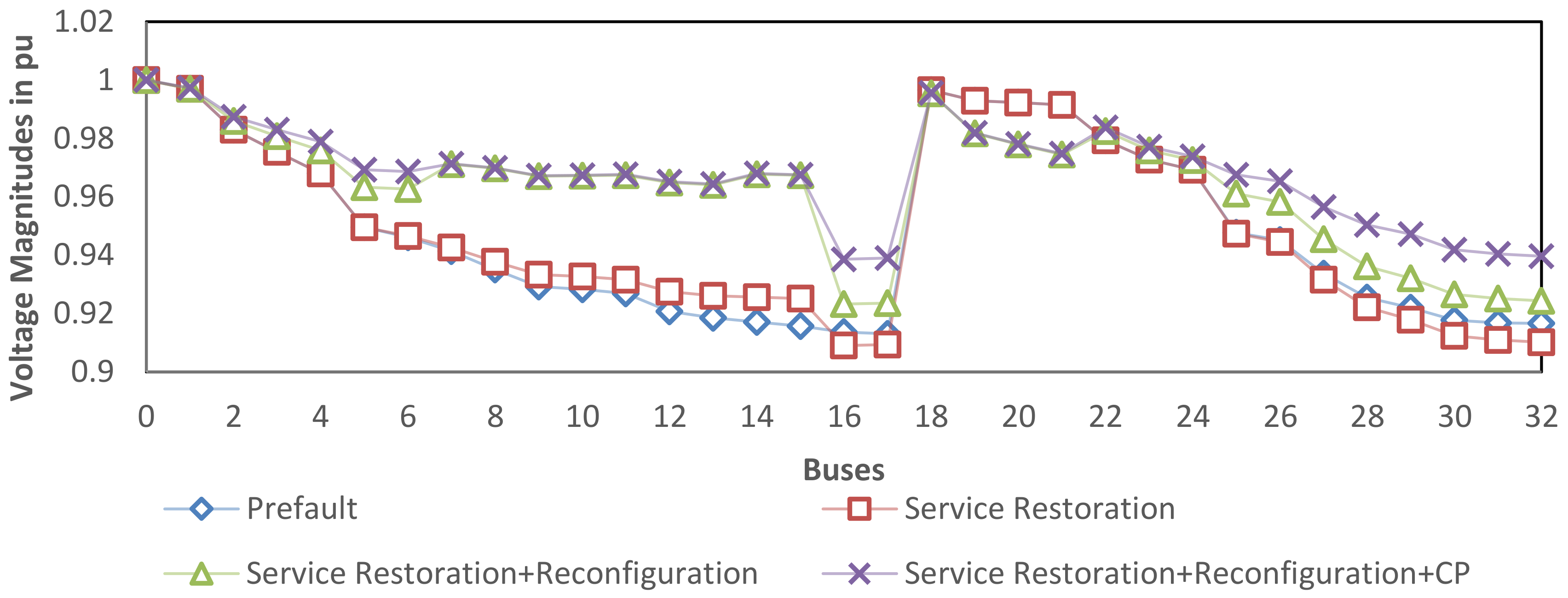
5.1. Test Case 1
5.1.1. Single Fault Condition (SFC)
5.1.2. Multiple Fault Condition (MFC)
5.1.3. Critical Fault Condition (CFC)
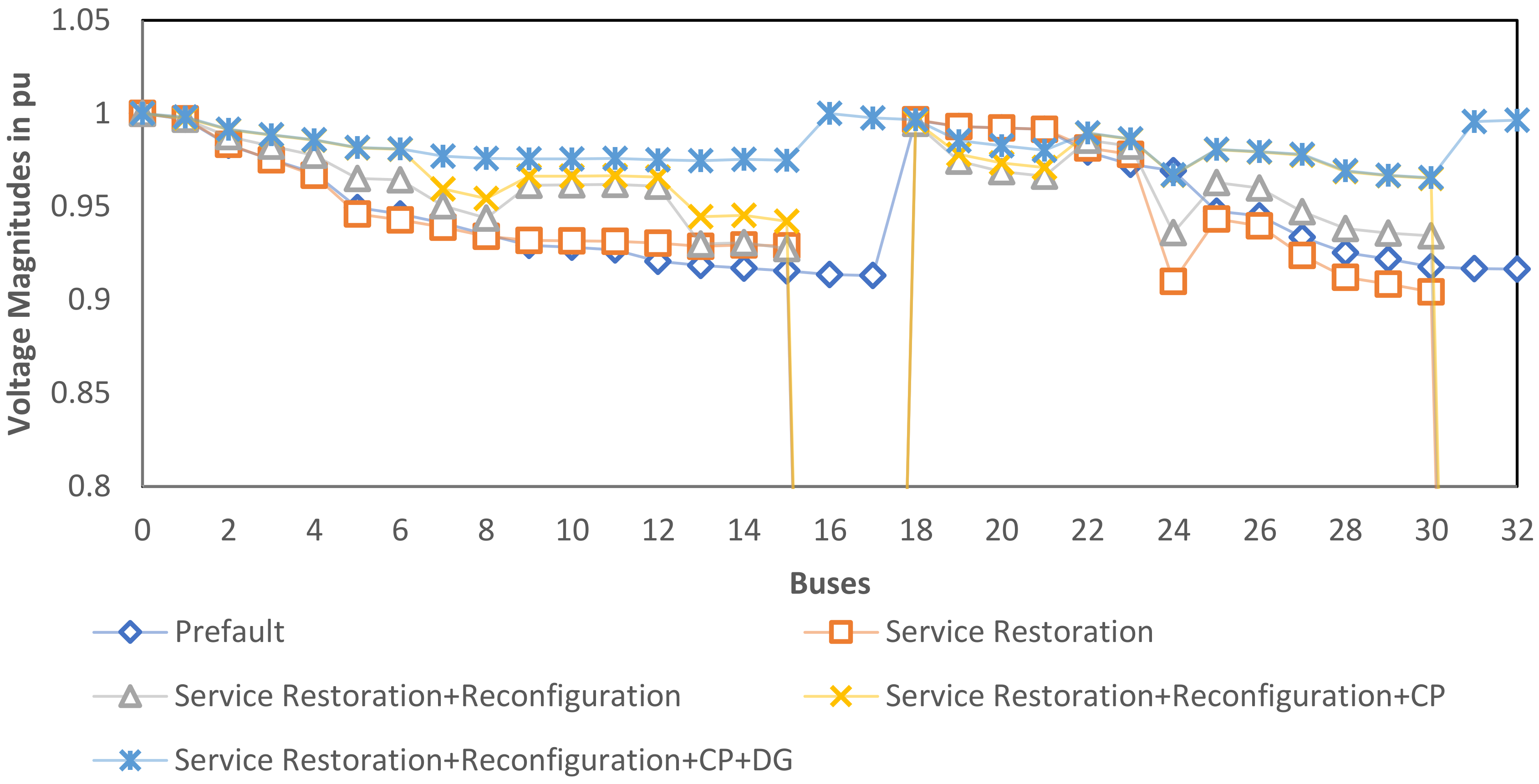
5.2. Test Case 2
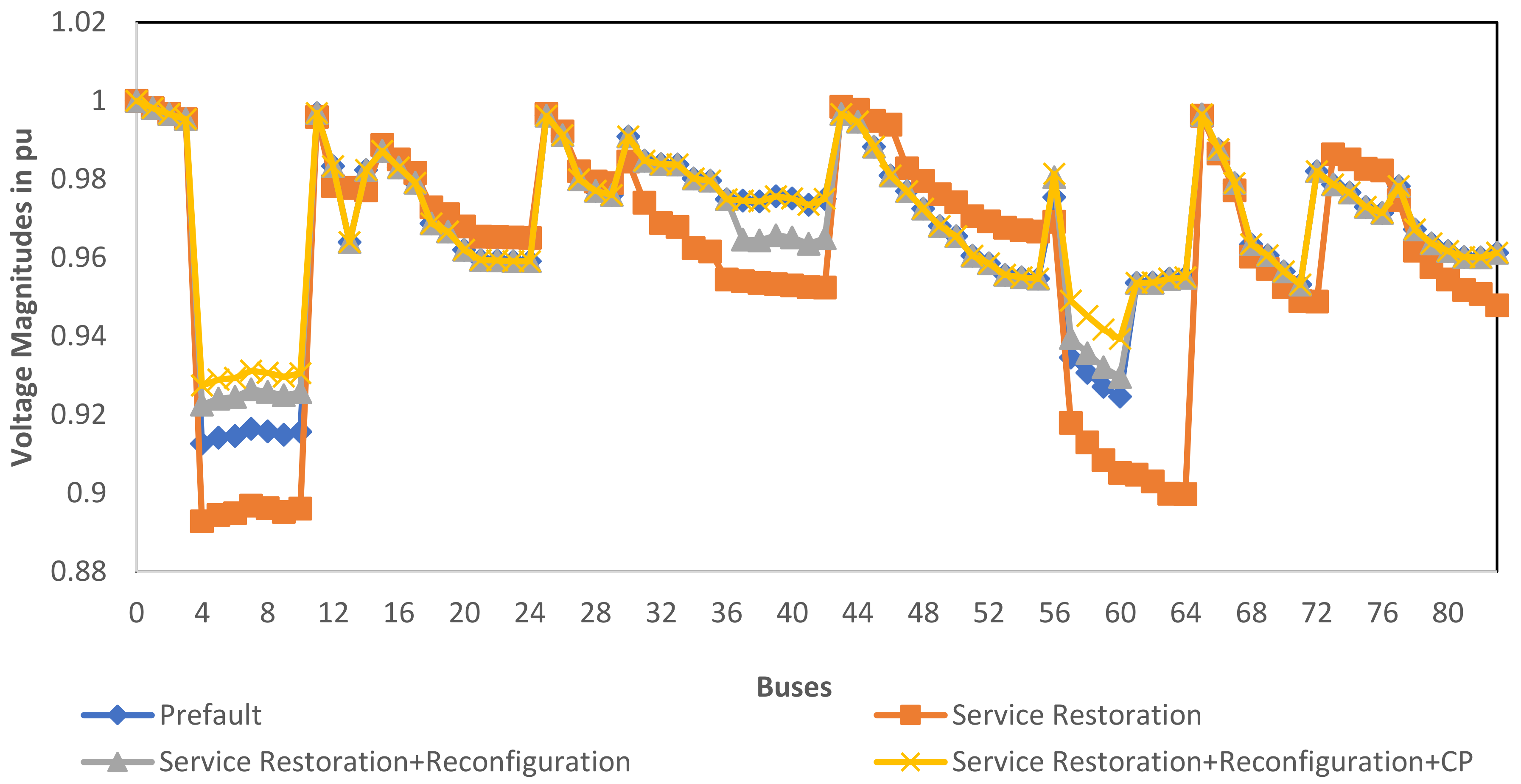
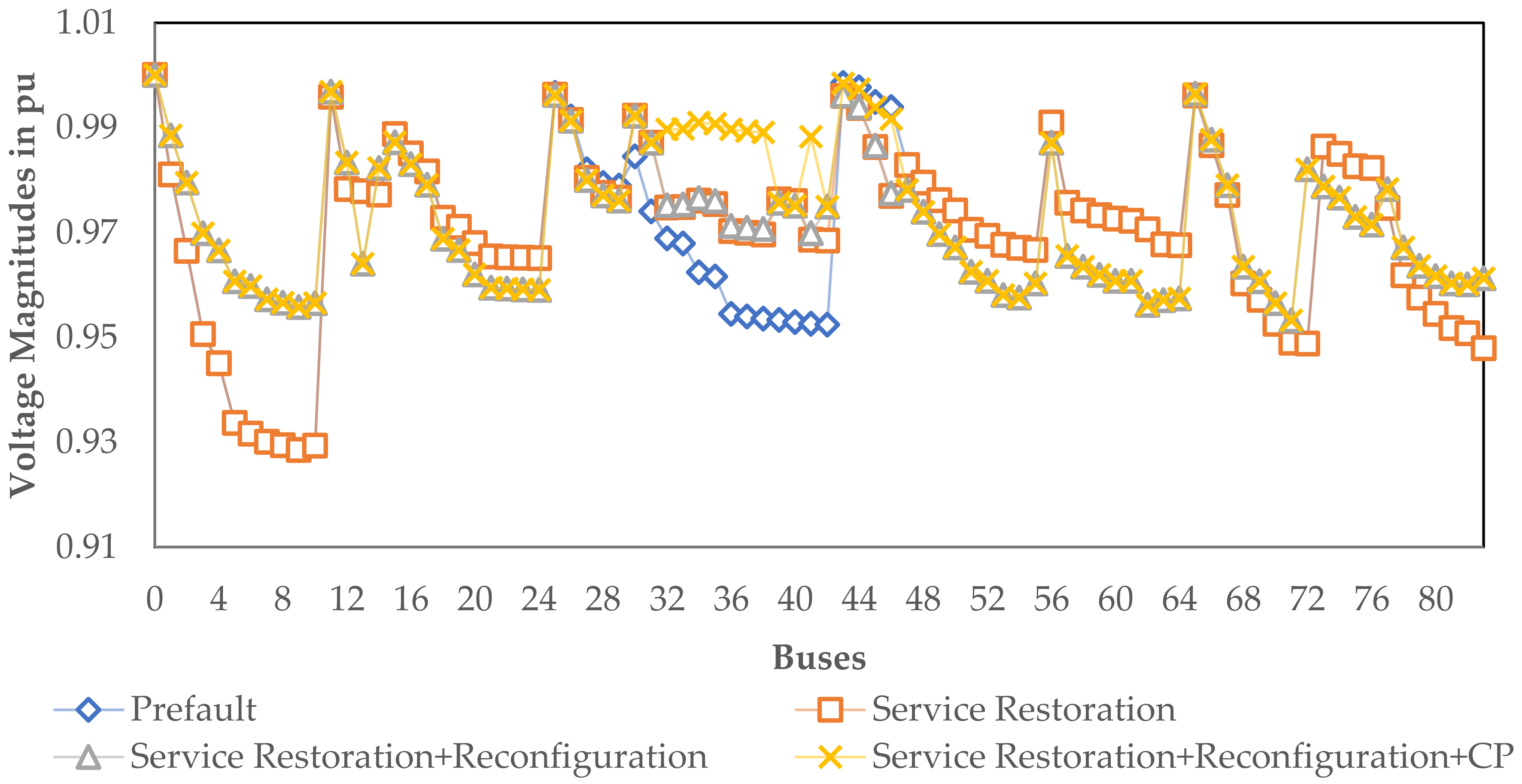
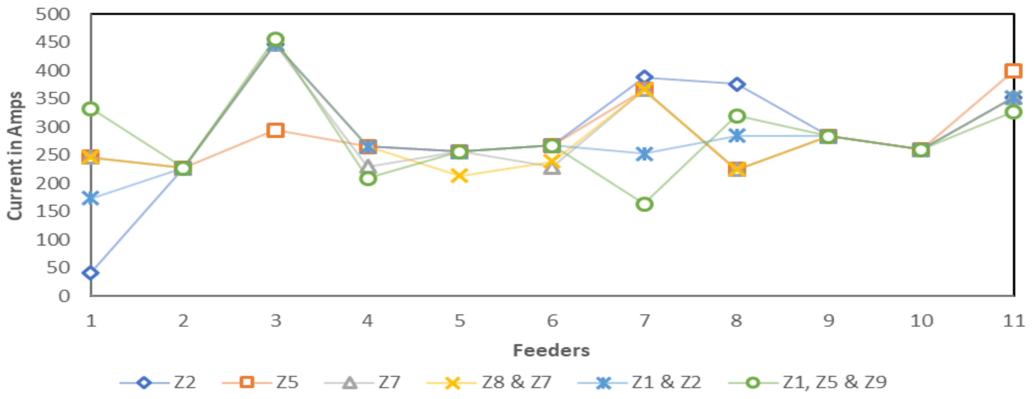
5.2.1. Single Fault Condition
5.2.2. Multiple Fault Condition
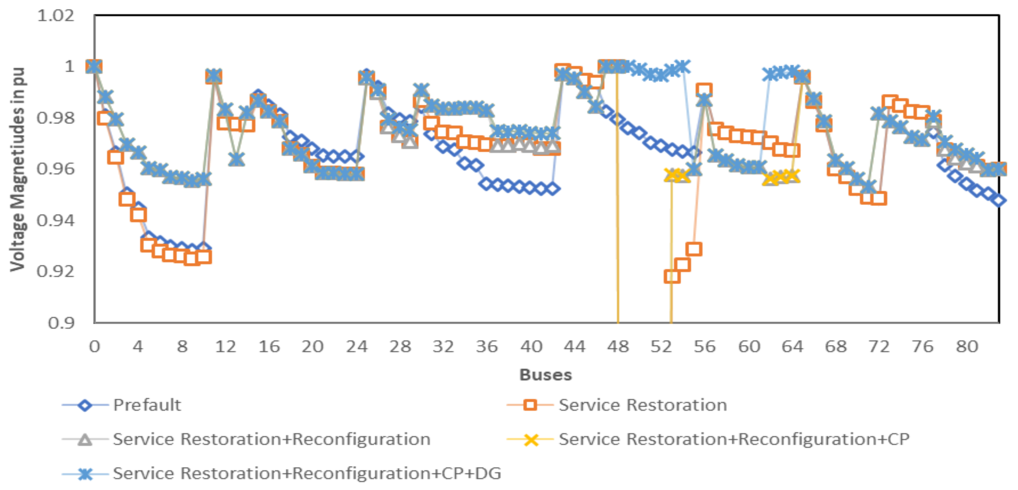
5.2.3. Critical Fault Condition
6. Conclusions and Future Work
Author Contributions
Funding
Acknowledgments
Conflicts of Interest
Abbreviations
| CA | control agent |
| CC | capacitor cost |
| CFC | critical fault condition |
| CP | capacitor placement |
| DER | distributed energy restoration |
| DG | distributed generators |
| DGC | DG cost |
| DSR | distribution system restoration |
| ELC | energy loss cost |
| EVs | electric vehicles |
| LDC | load dispatch center |
| MFC | multiple fault condition |
| MISOCP | mixed-integer second-order cone programming |
| MV | medium voltage |
| NCs | normally closed switches |
| Nos | normally open switches |
| RDS | radial distribution system |
| SFC | single fault condition |
| SRC | service restoration cost |
| TLA | teaching–learning algorithm |
| V2G | vehicle-to-grid |
Indices
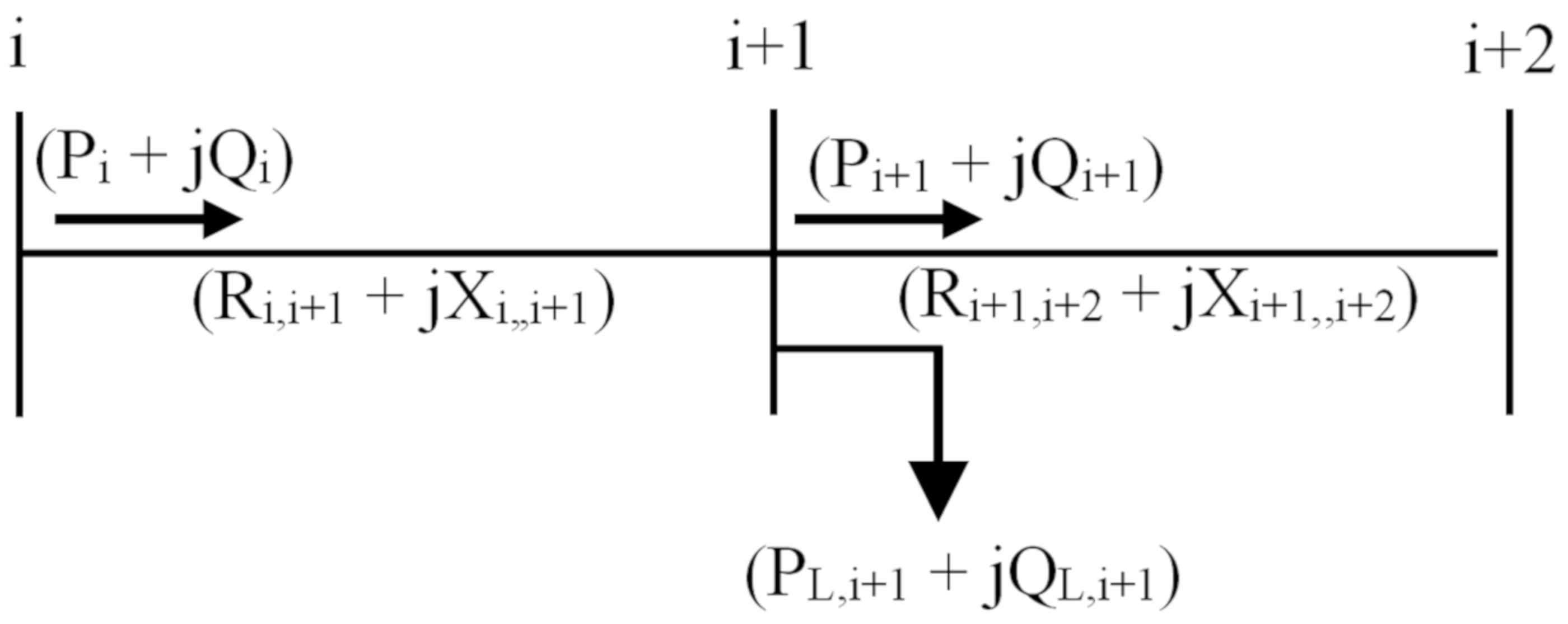
| . | Real and reactive powers that flow out of bus “i” |
| Real and reactive load powers in bus “i + 1” | |
| Resistance and reactance of the line section between buses “i” and “i + 1” | |
| Resistance and reactance of the line section between buses “i + 1” and “i + 2” | |
| Vi and Vi+1 | Voltage at ith and (i + 1)th bus |
| Ploss | Real power transmission loss of the system |
| nl | Total number of transmission lines of the distribution system |
| Real and reactive power demand | |
| PGj and QGj | Real and reactive power generation of jth DG |
| PGj,max and QGj,max | Maximum real and reactive power generation of ith DG |
| Vmin and Vmax | Minimum and maximum bus voltage |
| Ij | Current at jth branch |
| Imax | Maximum current |
| Minimum and maximum frequency | |
| Kp | Equivalent annual cost of power loss in $/(kW-year) |
| Cq,fixed | Fixed cost for the capacitor placement $/year |
| Annual cost for the capacitor installation in $/(kVAR-year) of ith bus | |
| Qcapacitor | Capacitor reactive power in (kVAR) |
| DGcost | Operating cost of DG in $/kW |
| ai, bi and ci | Cost coefficients of ith DG cost function |
References
- Baran, M.E.; Wu, F.F. Network reconfiguration in distribution systems for loss reduction and load balancing. IEEE Trans. Power Del. 1989, 4, 1401–1407. [Google Scholar] [CrossRef]
- Thiruvenkadam, S.; Nirmalkumar, A.; Sakthivel, A. MVC architecture-based Neuro-Fuzzy approach for distribution feeder reconfiguration for Loss reduction and load balancing. In Proceedings of the 2008 IEEE/PES Transmission and Distribution Conference and Exposition, Chicago, IL, USA, 21–24 April 2008. [Google Scholar]
- Wang, C.; Cheng, H.Z. Optimization of Network configuration in Large distribution systems using plant growth simulation algorithm. IEEE Trans. Power Syst. 2008, 23, 119–126. [Google Scholar] [CrossRef]
- Rao, R.S.; Narasimham, S.V.L.; Raju, M.R.; Rao, A.S. Optimal Network Reconfiguration of Large-Scale Distribution System Using Harmony Search Algorithm. IEEE Trans. Power Syst. 2011, 26, 1080–1088. [Google Scholar]
- Fereidunian, H.; Lesani, C. Lucas, Distribution System Reconfiguration Using Pattern Recognizer Neural Networks. Int. J. Eng. (Ije) Trans. B Appl. 2012, 15, 135–144. [Google Scholar]
- Pegado, R.; Naupari, Z.; Molina, Y.; Castillo, C. Radial distribution network reconfiguration for power losses reduction based on improved selective BPSO. Electr. Power Energy Syst. 2019, 169, 206–213. [Google Scholar] [CrossRef]
- Devi, V.S.; Anandalingam, G. Optimal restoration of power supply in large distribution systems in developing countries. IEEE Trans. Power Del. 1995, 10, 430–438. [Google Scholar] [CrossRef] [Green Version]
- Singh, S.P.; Raju, G.S.; Rao, G.K.; Afsari, M. A heuristics method for feeder reconfiguration and service restoration in distribution networks. Electr. Power Energy Syst. 2009, 31, 309–314. [Google Scholar] [CrossRef]
- Song, I.K.; Jung, W.W.; Kim, J.Y.; Yun, S.Y.; Choi, J.H.; Ahn, S.J. Operation Schemes of Smart Distribution Networks with Distributed Energy Resources for Loss Reduction and Service Restoration. IEEE Trans. Smart Grid 2013, 4, 367–374. [Google Scholar] [CrossRef]
- Li, J.; Ma, X.Y.; Liu, C.C.; Schneider, K.P. Schneider, Distribution System Restoration with Microgrids Using Spanning Tree Search. IEEE Trans. Power Syst. 2014, 29, 3021–3029. [Google Scholar] [CrossRef]
- Dimitrijevic, S.; Rajakovic, N. Service Restoration of Distribution Networks Considering Switching Operation Costs and Actual Status of the Switching Equipment. IEEE Trans. Smart Grid 2015, 6, 1227–1232. [Google Scholar] [CrossRef]
- Elmitwally, A.; Elsaid, M.; Elgamal, M.; Chen, Z. A Fuzzy-Multiagent Service Restoration Scheme for Distribution System with Distributed Generation. IEEE Trans. Sustain. Energy 2015, 6, 810–821. [Google Scholar] [CrossRef]
- Sharma, A.; Srinivasan, D.; Trivedi, A. A Decentralized Multiagent System Approach for Service Restoration Using DG Islanding. IEEE Trans. Smart Grid 2015, 6, 2784–2793. [Google Scholar] [CrossRef]
- Wang, S.; Chiang, H.D. Multi-objective service restoration of distribution systems using user-centered methodology. Electr. Power Energy Syst. 2016, 80, 140–149. [Google Scholar] [CrossRef] [Green Version]
- Huang, X.; Yang, Y.; Taylor, G.A. Service Restoration of Distribution Systems under Distributed Generation Scenarios. Csee J. Power Energy Syst. 2016, 2, 43–50. [Google Scholar] [CrossRef]
- Wang, F.; Chen, C.; Li, C.; Cao, Y.; Li, Y.; Zhou, B.; Dong, X. A Multi-Stage Restoration Method for Medium-Voltage Distribution System with DGs. IEEE Trans. Smart Grid 2017, 8, 2627–2636. [Google Scholar] [CrossRef]
- Thurner, L.; Scheidler, A.; Probst, A.; Braun, M. Heuristic optimisation for network restoration and expansion in compliance with the single contingency policy. IET Gener. Transm. Distrib. 2017, 11, 4264–4273. [Google Scholar] [CrossRef]
- Chen, B.; Chen, C.; Wang, J.; Butler-Purry, K.L. Sequential Service Restoration for Unbalanced Distribution Systems and Microgrids. IEEE Trans. Power Syst. 2018, 33, 1507–1520. [Google Scholar] [CrossRef]
- Sharma, A.; Trivedi, A.; Srinivasan, D. Multi-stage restoration strategy for service restoration in distribution systems considering outage duration uncertainty. IET Gener. Transm. Distrib. 2018, 12, 4319–4326. [Google Scholar] [CrossRef]
- Arif, A.; Wang, Z.; Wang, J.; Chen, C. Power Distribution System Outage Management with Co-Optimization of Repairs, Reconfiguration, and DG Dispatch. Trans. Smart Grid 2018, 9, 4109–4118. [Google Scholar] [CrossRef]
- Riahinia, S.; Abbaspour, A.; Moeini-Aghtaie, M.; Khalili, S. Load service restoration in active distribution network based on stochastic approach. IET Gener. Transm. Distrib. 2018, 12, 3028–3036. [Google Scholar] [CrossRef]
- Khederzadeh, M.; Zandi, S. Enhancement of Distribution System Restoration Capability in Single/Multiple Faults by Using Microgrids as a Resiliency Resource. IEEE Syst. J. 2019, 13, 1796–1803. [Google Scholar] [CrossRef]
- Sekhavatmanesh, H.; Cherkaoui, R. Analytical Approach for Active Distribution Network Restoration Including Optimal Voltage Regulation. IEEE Trans. Power Syst. 2019, 34, 1716–1728. [Google Scholar] [CrossRef] [Green Version]
- Hossan, M.S.; Chowdhury, B. Data-Driven Fault Location Scheme for Advanced Distribution Management Systems. IEEE Trans. Smart Grid 2019, 10, 5386–5396. [Google Scholar] [CrossRef]
- Aftab, M.A.; Hussain, S.S.; Ali, I.; Ustun, T.S. IEC 61850 based substation automation system: A survey. Electr. Power Energy Syst. 2020, 120, 106008. [Google Scholar] [CrossRef]
- Srinivasas Rao, R.; Narasimham, S.V.L.; Ramalingaraju, M. Optimal Capacitor Placement in A Radial Distribution System using Plant Growth Simulation Algorithm. Electr. Power Energy Syst. 2011, 33, 1133–1139. [Google Scholar]
- Rao, R.V.; Savsani, V.J.; Vakharia, D.P. Teaching–learning-based optimization: A novel method for constrained mechanical design optimization problems. Comput. Aided Des. 2011, 43, 303–315. [Google Scholar] [CrossRef]
- Rao, R.V.; Savsani, V.J.; Vakharia, D.P. Teaching–learning-based optimization: A novel optimization method for continuous non-linear large-scale problems. Inf. Sci. 2011, 183, 1–15. [Google Scholar] [CrossRef]


| References | Techniques Adapted | Scalability | Robustness | SRC | Optimization | Complexity | ||||
|---|---|---|---|---|---|---|---|---|---|---|
| Small | Medium | Large | SFC | MFC | CFC | |||||
| [11] | Reconfiguration | C | C | C | C | NC | NC | C | NC | Less |
| [12] | Reconfiguration + DG | C | NC | NC | C | NC | C | NC | NC | Moderate |
| [13] | DG + V2G | C | C | C | NC | NC | C | NC | NC | Moderate |
| [16] | Reconfiguration + DG | C | C | NC | C | C | NC | NC | NC | Moderate |
| [17] | Reconfiguration | C | C | C | C | C | NC | C | NC | Large |
| [19] | DG | C | C | C | C | C | C | NC | NC | Less |
| [20] | Reconfiguration + DG | C | C | C | C | C | C | NC | NC | Large |
| Proposed | Reconfiguration + CP + DG | C | C | C | C | C | C | C | C | Less |
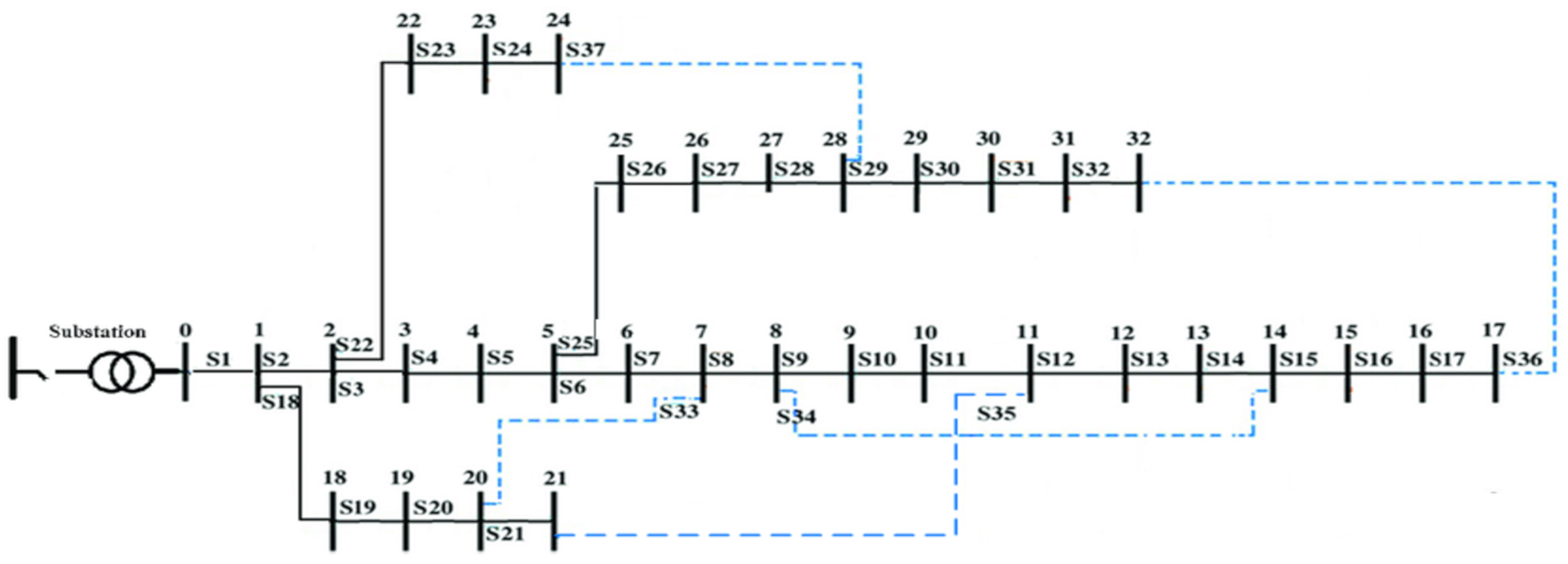
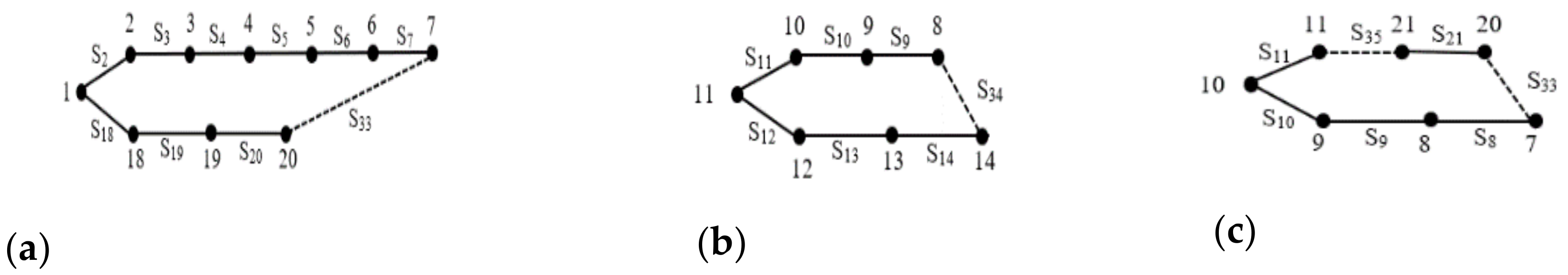
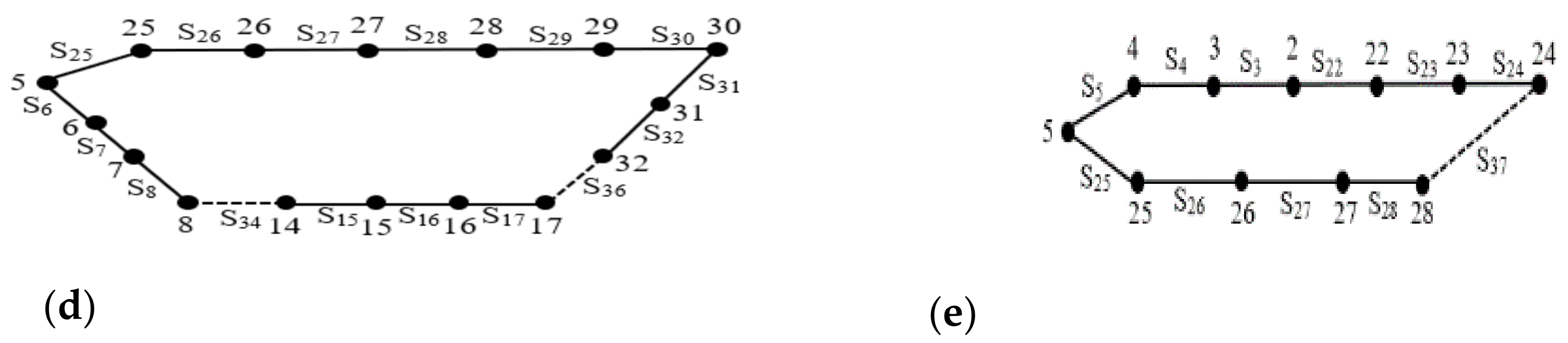
| Zone (Z) | Normally Closed Switches (NCs) | Normally Open Switches (NOs) |
|---|---|---|
| 1 | S4, S5, S6, S7, S19, S20 | S33 |
| 2 | S12, S13, S14 | S34 |
| 3 | S8, S9, S10, S11, S21 | S35 |
| 4 | S15, S16, S17, S29, S30, S31, S32 | S36 |
| 5 | S23, S24, S25, S26, S27, S28 | S37 |
| Faulted Zone | Faulted Switch | Normally Open Switches | Optimal Location of Capacitor | Q in kVAR | Postfault before Optimization | Postfault after Optimization | % Saving | ||
|---|---|---|---|---|---|---|---|---|---|
| Minimum Bus Voltage in pu | Energy Loss Cost in $ | Minimum Bus Voltage in pu | SRC in $ | ||||||
| 1 | S5 | S5, S10, S28, S34, S36 | 5 | 450 | 0.8378 | 57,969.54 | 0.9389 | 27,030.26 | 53.37 |
| 2 | S12 | S7, S9, S12, S32, S37 | 14 | 300 | 0.9167 | 33,152.44 | 0.9379 | 24,250.46 | 26.85 |
| 3 | S8 | S8, S14, S28, S32, S33 | 11 | 700 | 0.9297 | 25,786.38 | 0.9406 | 24,888.02 | 3.48 |
| 4 | S26 | S7, S9, S14, S26, S32 | 23 | 300 | 0.9300 | 30,246.10 | 0.9410 | 24,050.27 | 20.48 |
| 5 | S16 | S7, S9, S14, S16, S37 | 29 | 900 | 0.9090 | 34,273.78 | 0.9501 | 19,321.30 | 43.63 |
| Faulted Zone | Faulted Switches | Normally Open Switches | Optimal Location of Capacitor | Q in kVAR | Postfault before Optimization | Postfault after Optimization | % Saving | ||
|---|---|---|---|---|---|---|---|---|---|
| Minimum Bus Voltage in pu | Energy Loss Cost in $ | Minimum Bus Voltage in pu | SRC in $ | ||||||
| 1 & 3 | S5 & S10 | S5, S10, S28, S34, S36 | 5,11 | 450 750 | 0.8528 | 48,036.70 | 0.9579 | 27,467.61 | 42.82 |
| 2 & 5 | S14 & S31 | S7, S9, S14, S31, S37 | 14,29 | 300 900 | 0.9051 | 33,742.64 | 0.9681 | 18,715.66 | 44.53 |
| 1,2 & 4 | S6, S14 & S24 | S6, S9, S14, S24, S32 | 14, 19, 27 | 900,600 1800 | 0.9213 | 32,175.71 | 0.9762 | 26,968.99 | 16.18 |
| Sl. No. | Line Number | Affected Zone | Fault Category |
|---|---|---|---|
| 1 | 13 | Z2 | Faulted zone |
| 2 | 16 | Z4 | Critical zone |
| 3 | 24 | Z5 | Faulted zone |
| 4 | 31 | Z4 | Critical zone |
| Before Restoration | After Restoration | |||
|---|---|---|---|---|
| Unserved Loads | Unserved Loads | CP Location | DG Location | SRC in $ |
| 16, 17, 31 and 32 | - | 14 & 27 | 16 | 34,652.02 |
| Fault Conditions | Faulted Zone | Faulted Switch | Optimal Location of Capacitor + DG | Value Q in kVAR | Postfault before Optimization | Postfault after Optimization | % Saving | ||
|---|---|---|---|---|---|---|---|---|---|
| Minimum Bus Voltage in Pu | Energy Loss Cost in $ | Minimum Bus Voltage in Pu | SRC in $ | ||||||
| SFC | Z2 | 4 | 57 | 900 | 0.8928 | 110,958.84 | 0.9274 | 91,244.70 | 17.77 |
| Z7 | 37 | 29 | 1850 | 0.9285 | 89,483.27 | 0.9531 | 78,882.78 | 11.85 | |
| Z5 | 20 | 78 | 3150 | 0.9175 | 97,377.49 | 0.9520 | 80,813.86 | 17.01 | |
| MFC | Z8 Z7 | 32 39 | 46 36 | 450 1350 | 0.9285 | 87,027.61 | 0.9531 | 79,426.26 | 8.73 |
| Z1 Z2 | 54 6 | 51 57 | 1650 3300 | 0.9096 | 99,263.97 | 0.9531 | 77,659.92 | 21.76 | |
| Z1 Z5 Z9 | 42 53 82 | 42 53 78 | 600 300 2100 | 0.9014 | 106,541.56 | 0.9383 | 87,788.26 | 17.60 | |
| Zone | Critical Lines | Loads Connected |
|---|---|---|
| Zone 8 | 20–21, 21–22, 21–23, and 23–24 | 21, 22, 23, and 24 |
| Zone 13 | 7–8,7–9, and 7–10 | 8, 9, and 10 |
| Sl. No. | Start Bus | End Bus | Affected Zone | Fault Category |
|---|---|---|---|---|
| 1 | 36 | 37 | 10 | Faulted zone |
| 2 | 48 | 49 | 1 | Critical zone |
| 3 | 52 | 53 | 1 | Critical zone |
| 4 | 81 | 82 | 5 | Faulted zone |
| Before Restoration | After Restoration | |||
|---|---|---|---|---|
| Unserved Loads | Unserved Loads | CP Location | DG Location | SRC in $ |
| 50, 51 and 52 | - | 37 & 78 | 50 | 125,401.95 |
| Test Case | Fault Condition | Number of Learners Considered | Maximum Number of Iterations Considered | Number of Iterations Taken to Reach Optimal Solution | Execution Time in Msec. | ||
|---|---|---|---|---|---|---|---|
| Minimum | Maximum | Minimum | Maximum | ||||
| 1 | SFC | 25 | 50 | 23 | 28 | 482.69 | 559.29 |
| MFC | 50 | 50 | 26 | 34 | 864.94 | 890.45 | |
| CFC | 50 | 50 | 31 | 39 | 988.40 | 1003.05 | |
| 2 | SFC | 75 | 100 | 58 | 72 | 31,498.32 | 31,717.51 |
| MFC | 100 | 100 | 64 | 78 | 42,039.26 | 42,066.82 | |
| CFC | 100 | 100 | 73 | 84 | 42,268.46 | 43,172.34 | |
Publisher’s Note: MDPI stays neutral with regard to jurisdictional claims in published maps and institutional affiliations. |
© 2020 by the authors. Licensee MDPI, Basel, Switzerland. This article is an open access article distributed under the terms and conditions of the Creative Commons Attribution (CC BY) license (http://creativecommons.org/licenses/by/4.0/).
Share and Cite
S, T.; Ra, I.-H.; Kim, H.-J. Cost-Effective Outage Management in Smart Grid under Single, Multiple, and Critical Fault Conditions through Teaching–Learning Algorithm. Energies 2020, 13, 6205. https://doi.org/10.3390/en13236205
S T, Ra I-H, Kim H-J. Cost-Effective Outage Management in Smart Grid under Single, Multiple, and Critical Fault Conditions through Teaching–Learning Algorithm. Energies. 2020; 13(23):6205. https://doi.org/10.3390/en13236205
Chicago/Turabian StyleS, Thiruvenkadam, In-Ho Ra, and Hyung-Jin Kim. 2020. "Cost-Effective Outage Management in Smart Grid under Single, Multiple, and Critical Fault Conditions through Teaching–Learning Algorithm" Energies 13, no. 23: 6205. https://doi.org/10.3390/en13236205