A Mathematical Model of Biomass Combustion Physical and Chemical Processes

Abstract

The numerical simulation of biomass combustion requires a model that must contain, on one hand, sub-models for biomass conversion to primary products, which involves calculations for heat transfer, biomass decomposition rate, product fractions, chemical composition, and material properties, and on the other hand, sub-models for volatile products transport inside and outside of the biomass particle, their combustion, and the char reduction/oxidation. Creating such a complete mathematical model is particularly challenging; therefore, the present study proposes a versatile alternative—an originally formulated generalized 3D biomass decomposition model designed to be efficiently integrated with existing CFD technology. The biomass decomposition model provides the chemical composition and mixture fractions of volatile products and char at the cell level, while the heat transfer, species transport, and chemical reaction calculations are to be handled by the CFD software. The combustion model has two separate units: the static modeling that produces a macro function returning source/sink terms and local material properties, and the dynamic modeling that tightly couples the first unit output with the CFD environment independently of the initial biomass composition, using main component fractions as initial data. This article introduces the generalized 3D biomass decomposition model formulation and some aspects related to the CFD framework implementation, while the numerical modeling and testing shall be presented in a second article.

1. Introduction

Although the mathematical modeling of the thermal biomass conversion phenomena began as early as the 1940s, the progress of theoretical study of biomass thermal decomposition was relatively slow. The introduction of electronic computing systems combined with the development of experimental methods and apparatus brought some much-needed insight on the subject; however, undeniably, there is more improvement to be made still. The main reason for this situation is the outstanding complexity of the process itself: the amount and extent of physical and chemical processes and interactions characteristic to the thermal decomposition of biomass is simply overwhelming. The chemical transformations of the biomass main components, cellulose, hemicellulose, and lignin are governed by reaction mechanisms that have not been fully understood or described yet, either by theoretical or by experimental studies. For example, recent attempts to define kinetic-type mechanisms of increased complexity have demonstrated good accuracy, but their implementation is cumbersome and limited by the available computational resources. It is safe to say even that the full breadth and depth of this process will never get to be captured by mathematical modeling, but also that is equally debatable if such a level of modeling accuracy is really relevant. Nevertheless, the increasing demand for modeling of biomass thermal conversion in engineering applications must be fulfilled while taking into account the limitations of computing power and development time.

Under these circumstances, the mathematical modeling efforts, even of the more recent studies, are generally limited to the implementation of simple methods, which is based on the assumption that the biomass thermal decomposition might be well enough approximated by a few global reactions whose parameters can be determined experimentally. These methods are known as the kinetic modeling methods. The most extensively used form of kinetic modeling involves schemes with only a few reactions expressed as Arrhenius-type equations, especially due to the availability of well-proven and very easy to implement kinetic schemes. These have been tested against a wide range of experimental data and demonstrated acceptable accuracy from an engineering standpoint in predicting decomposition rates and product yields.

One very important and practically universal limitation of the current models for large biomass particles thermal decomposition is their formulation based on isolated particles of regulated shape (mostly spherical or cylindrical). Although this approach allows for a great simplification of the model’s equations due to the use of spherical (1D) or cylindrical (2D) coordinate systems, three-dimensional effects are always present in real-life applications, and quite often, they cannot be neglected. The non-uniformity of radiative or convective thermal loads, the inherent variability in external convective transport of product species and oxygen diffusion, the local or global effects of particle geometrical features and shape, and the mutual influence of clustered configurations are only some of the particularities that call for a true 3D modeling approach.

Taking all of this into consideration, the motivation of the present study was to identify a modeling procedure that is not only simple to implement, easy to use, and computationally efficient, but also sufficiently accurate for engineering design activities and with a spectrum of applications as broad as possible. The procedure devised herein consists of two main stages: the first stage is identified as the static modeling phase, which takes place outside of the actual simulation, with the purpose of generating the algorithm (macro functions) that supplies the CFD platform specific input data, and the second stage is the dynamic modeling phase, where the CFD model is bi-directionally coupled to the biomass decomposition model in the form of a User-Defined Function (UDF). The static modeling phase starts from a slightly modified Miller–Bellan kinetic scheme—although any other scheme could be utilized instead, simpler or more complex—retaining its main assumptions: (1) the biomass composition can be generally described as a homogeneous mixture of cellulose, hemicellulose, lignin, ash, and water, and (2) the superposition principle is valid with respect to the biomass decomposition process. The resulting subsequent derivation of the mathematical model is simple and efficient. The model’s output data contain the primary decomposition product fractions, the chemical composition of the volatile fractions, and the thermodynamic properties of all products and reactants, as functions of temperature only. An important feature of the derived mathematical model is the ability to generate not only the chemical composition of the primary gaseous mixture but also that of the secondary gaseous mixture resulting from tar thermal decomposition, both inside and outside of the particle volume, in the absence of which combustion simulation is not possible. The char residue gasification and combustion modeling process assume a temperature-dependent chemical composition equivalent to a mixture of carbon, hydrogen, and oxygen. The volatiles’ oxidation is accomplished using a simplified reaction mechanism that incorporates only the most relevant reactions due to the inherently high computational effort associated with combustion modeling in unsteady simulations.

2. State of the Art in Numerical Modeling of Biomass Decomposition

The traditional modeling of the biomass thermal decomposition was done by constructing heavily simplified mathematical models, which could be applied to basic geometric shapes and for certain operational conditions.

Biomass fuels are challenging because of the physical and chemical characteristics that affect the thermal conversion process and energy production efficiency [1,2]. Fundamental characterization and the detailed investigation of biomass fuels thermal decomposition under controlled conditions are the keys to understanding the complex phenomena occurring during (full-scale) thermal conversion processes.

Due to the limited understanding of the process, the initial attempts to mathematically model the biomass thermal decomposition proved quite challenging, which resulted in rather simple models [3]. The complexity of the physical and chemical transformations characterizing the thermal decomposition of biomass is so high that even if limiting the study to the devolatilization stage, it is practically impossible to define a complete and correct modeling approach.

2.1. Kinetic Modeling of Biomass Decomposition

Kinetic models are simplified decomposition schemes trying to approximate the real complex phenomenology using empirical global reactions. These reactions describe the conversion of biomass or its main components (cellulose—CL, hemicellulose—HCL, lignin—LG) to primary decomposition products—solid residue (char) and volatiles (gas and tar). The global reactions are most frequently approximated by first-order reactions, where the reaction rate, k, is expressed as a function of temperature, which is represented by an Arrhenius type Equation.

The main kinetic modeling approaches in the art can be classified into five categories: (1) Single global reaction modeling, (2) Multiple parallel reactions modeling, (3) Competitive reactions modeling, (4) Kinetic modeling based on the Distributed Activation Energy method (DAEM) [4,5,6], and (5) Hybrid modeling using different combinations of kinetic models of type (2) and (3) [7,8]. The most promising approaches for future development appear to be the models of type (4) and (5).

The most relevant kinetic mechanisms developed by different authors are (1) the Broido–Shafizadeh scheme [9,10], (2) the Koufopanos–Srivastava scheme [11,12,13], and (3) the Thurner and Man scheme [14]. The hybrid scheme developed by Ranzi et al. must also be mentioned as one of the highest complexity kinetic schemes available in the literature, which was later enhanced by Gauthier et al. [15].

The Miller–Bellan scheme, published in 1997, is one of the few mechanisms for biomass thermal decomposition intended to have general applicability [7]. Based on the effects of superposition assumption, it is a hybrid scheme, with parallel decomposition of the main components through competitive reactions. There were some recent attempts to improve this mechanism by Blondeau et al. in 2011 [8]. Considering all the advantages offered by the Miller–Bellan scheme, it has also been adopted in [16].

2.2. Eulerian–Lagrangian Approach of Gas–Solid Hydrodynamics in Biomass Reactors

Additionally, in the last two decades, significant research efforts have been devoted to the development of numerical models to study the complex hydrodynamics of gas–solid flows in biomass reactors [17]. A good understanding of the hydrodynamic behavior of such systems is important for the design and scale up of new efficient reactors. When employing the Eulerian–Lagrangian approach, the gas is treated as continuous phase and particles are treated as discrete phase. The trajectories of individual particles are tracked in space and time by directly integrating the equation of motion while accounting for interactions with other particles, walls, and the continuous phase. This approach has been much utilized for simulating coal-powered combustion systems, but less published work is to be found for biomass reactors. However, recent model developments have proven promising with good correlations to experimental work on fluidized bed bioreactors [18]. However, a significant challenge arises when such multi-phase flow simulations are combined with realistic and comprehensive kinetic models as described above. This is not only a very physically and chemically complex system to model correctly but necessitates also sophisticated numerical schemes in order to overcome the very high computational requirements.

2.3. Isolated Particle Decomposition Modeling

Most existing numerical models of biomass thermal decomposition are applicable for studying the physical and chemical phenomena associated with a single particle. One of the reasons justifying this approach is that the experimental investigation of an isolated particle is easier to handle than the processes occurring in an entire furnace. From a scientific point of view, it is also safe to assume that the complete understanding of the real phenomenology and the correct numerical modeling of a small isolated particle will implicitly lead to improved calculation methods to be used in industrial applications involving a large number of particles, such as the fixed bed or fluidized bed reactors.

Several extensive reviews of numerical modeling of biomass decomposition are available, including those of Moghtaderi [19] and Di Blasi [20]. According to their work, the existing models can be classified into three main categories based on dimensional complexity:

-

1D models: Originally developed by Bamford et al. in 1946 [3], the one-dimensional model was further improved by Koufopanos et al. [21], Babu and Chaurasia [22,23], Fan et al. [24], Di Blasi and Galgano [25], Villermaux et al. [26], and Bellais et al. [27];

-

2D models: One of the most complete 2D models was published by Di Blasi in 1998 [28]; recently, Blondeau and Jeanmart [29] published a study on such a model;

-

3D models: There are very few 3D models, for example, the model developed by Yuen et al. [30] and the Park model [31] presented in his doctoral thesis (2008).

Some of these models are quite complex and well-performing, but unfortunately, most of them are limited to the drying and devolatilization phases, and only some can be used to quantify the char decomposition phase, too. However, none of these models is capable of in-depth simulation of all the phases associated to biomass combustion. A recent, one-dimensional approach published by Mehrabian et al. [32] covers also the volatiles combustion phase, but it is limited to small, simple-shaped particles.

3. General Combustion Model Overview

As a result of the complex physical and chemical reactions involved in biomass pyrolysis and combustion processes, it is impossible, for the moment at least (with the computational resources available), to address the issue without making certain simplifications. Consequently, two main assumptions have been formulated and used in the development of the numerical model:

(1)

Regardless of origin, all biomass types can be considered as a homogenous mixture of cellulose, hemicellulose, lignin (with three main variations), ash, and water. This idea is supported by technical analysis performed for most biomass sources of practical interest;

(2)

The kinetic model is based on the superposition principle: the biomass decomposition is a linear combination of the three major components decomposition effects, i.e., cellulose (CL), hemicellulose (HCL), and lignin (LG). The three sets of reactions occur in parallel, without influencing each other, irrespective of the pyrolysis conditions. The model presented here is based on a slightly modified Miller and Bellan kinetic scheme, which is one of the few generalized pyrolysis decomposition models [7].

In addition to the Miller and Bellan kinetic scheme, this study considers the initial moisture by means of a separate reaction. The complete kinetic scheme is shown in Figure 1, and the kinetic constants of the Miller and Bellan model are given in

Table 1. Kinetic constants of modified Miller and Bellan model [7].

Reaction	Cellulose	Hemicellulose	Lignin
k1	2.80 × 1019exp (−242.4/RT)	2.10 × 1016exp (−186.7/RT)	9.60 × 108exp (−107.6/RT)
k2	3.28 × 1014exp (−196.5/RT)	8.75 × 1015exp (−202.4/RT)	1.50 × 109exp (−143.8/RT)
k3	1.30 × 1010exp (−150.5/RT)	2.60 × 1011exp (−145.7/RT)	7.70 × 106exp (−111.4/RT)
X	0.35	0.6	0.75
k4	4.28 × 106exp (−108.0/RT)

.

In addition to these two assumptions, the present study has established two properties for the global combustion model:

(1)

It should exhibit such a degree of comprehensiveness that it can be applied to an extensive range of biomass sources with acceptable accuracy without the need for structural or conceptual changes;

(2)

Given the 3D modeling complexity involved, it should be designed in such a way as to require a reasonable calculation effort while its applicability should also include industrial design.

The approach used in most of the existing biomass thermal decomposition models is the development, alongside the thermal decomposition model, of a numerical framework to solve the model equation system.

The aim of this study was to create a model that is comprehensive enough to approach the problem of biomass thermal decomposition while simultaneously including the combustion stage. This implies the ability to simulate both the convection and diffusivity of chemical species in the space around biomass particles and chemical reactions between them throughout the area of interest, plus the dynamic and thermal effects associated with these processes.

The achieved solution consists in the integration/coupling of existing fluid dynamics software with a separate model implemented by an external procedure introducing all the required additional elements in the mathematical and numerical CFD software framework. This integration allows the use of all relevant and available CFD software features, thereby significantly reducing the programming effort.

Among the CFD physical modeling features that have streamlined the global model development, the porous media model is worth mentioning. Obviously, it was the basis for the external thermal decomposition model, allowing direct coupling, including at the equation system level, of solid and volatile fraction parameters and mass transfer (from solid to fluid) and energy (both ways).

The resulting numerical model is basically complete, the amount and impact of simplifications or current limitations being sufficiently low, as suggested by the numerical tests.

4. Biomass Physical Properties Modeling

Biomass is a very complex, inhomogeneous, and anisotropic material and any attempt to numerically represent its exact inner structure and material properties is practically impossible. However, some simplifying assumptions can be made taking into account the scale of decomposition processes in specific systems and the typical size of a biomass particle.

The main material properties considered for biomass modeling, the assumptions and simplifications underlying the mathematical correlations used, and their transfer to the CFD numerical model are presented below.

4.1. Biomass Density and Shrinkage

The cell-wall density of woody biomass was determined to be effectively constant for all types of woods considered. Studies such as [2] and [3] suggest a value of 1530 kg/m³, which was also adopted in this study. Other bibliographic sources mention a value within 1450–1500 kg/m³. Based on this assumption, density variation in natural, dry woods is a consequence of the variation in the total volume of structural voids, pores, and intracellular channels. Conventionally, cell-wall density was considered as effective or reference biomass density (${\rho }_{ef}$), and the density determined by established methods based on biomass volume and weight in a certain state was considered as apparent density. Consequently, using the effective density, which is invariable with biomass conversion processes, all dependent variables can be more easily determined.

During devolatilization, the particle continuously loses mass, and its apparent density and porosity change. In fact, a change (usually a reduction) in particle volume occurs along with biomass drying and decomposition, which is process called “particle contraction”. Subsequently, during char combustion, the particle mass loss rate amplifies even further. Particle volume after each conversion stage depends on several parameters, including initial density (hardwood loses less volume compared to softwood), decomposition conditions (that may influence, for example, the amount of char), ash content, etc.

In a first stage, the change in particle volume occurs because of water loss (biomass drying). During the second stage, biomass loses volume due to structural changes that occur during devolatilization. In the char combustion stage, volume reduction occurs almost exclusively due to oxidation reactions accompanied by the decomposition and oxidation of non-volatile residues, containing hydrogen and oxygen in addition to carbon. The final volume essentially corresponds to ash, namely inorganic salts from biomass initial composition.

The current version of the numerical combustion model does not explicitly include contraction, the discretization mesh remaining fixed. Considering previous research findings [5,10] and the idea that material property with the highest impact on numerical model results is char thermal conductivity, the lack of contraction was compensated by scaling conductivity measured experimentally by a factor equal to the ratio of the apparent char density determined experimentally and the apparent density obtained by numerical simulation.

The concept of concentration is used instead of density in all three components of the combustion model, which is numerically equivalent, and the unit and notation are identical ($\rho$,kg/m³). The initial concentration calculation of solid biomass constituents is done using the apparent density of dry biomass (${\rho }_{db}$) and the corresponding fractions from biomass technical analysis, which are used as model inputs. For example, the initial cellulose concentration is:

$${\rho }_{CL}={\rho }_{db} Y_{CL}$$

(1)

Initial fractions of other components are determined similarly.

Subsequent concentration changes of solid components (CL, HCL, and LG under stable form, then active form, and finally char) depend only on the thermal decomposition (volume being fixed) and are determined using appropriate Equations (22)–(24), according to the Miller–Bellan kinetic scheme.

Biomass reference density (${\mathsf{\rho }}_{\mathrm{ef}}$) is effectively used in a CFD numerical model only to estimate the solid thermal capacity or solid mass calculation, knowing the volume of each individual cell in the computational mesh; then, the result is weighted with the local porosity value. This applies at any time step, even during biomass thermal decomposition, because the above calculation uses current porosity, which is continuously updated by the following equation:

$$\mathsf{\phi }\left(\mathrm{t}\right)=1-\frac{{\sum }_{\mathrm{x}}{\mathrm{C}}_{\mathrm{x}}\left(\mathrm{t}\right)}{{\mathsf{\rho }}_{\mathrm{ef}}}$$

(2)

where the numerator is the sum of solids concentrations (CL, HCL, and LG under stable and active form—x variables, plus char concentration and finally, ash, all local values). Given the biomass volume invariability, the solid mass is calculated by the equation:

$$m_s\left(t\right)= \left[1-\phi \left(t\right)\right]{\rho }_{ef} V_{cel}$$

(3)

where $V_{cel}$ is cell volume (control volume in the computational mesh).

4.2. Thermal Conductivity

As demonstrated experimentally, the thermal conductivity coefficient varies significantly with temperature in all phases. Thermal conductivity values of solids and volatiles are required by the CFD numerical model to assess the heat balance at each time step.

By means of the UDF transfer function, any mathematical relation modeling the thermal conductivity function of temperature may be implemented. Due to the associated flexibility, this method was generally preferred over the alternatives already implemented in the CFD platform, with few exceptions.

4.2.1. Volatiles Thermal Conductivity

Since the thermal conductivity impact of volatiles is generally low (gas thermal conductivity is at least one order of magnitude lower than solids, and the main mechanism of gas heat transfer is convection, particularly in the case of turbulent flow), only constant values—specified individually for each chemical species—have been used, in order to simplify the numerical model.

Volatiles conductivity increases with temperature, but for the maximum temperatures observed during biomass thermal decomposition, conductivity values do not exceed 0.05–0.07 W/m/K for most species listed, condensable fractions included (except hydrogen, which is found in small and unnoticeable amounts).

4.2.2. Thermal Conductivity of Raw Biomass

As for solids, several empirical correlations from experimental measurements of thermal conductivity are available in the literature. Most such correlations are applicable for raw biomass and char. Raw biomass data have been measured at low temperatures, generally not exceeding 100 °C (except [6], where maximum temperature was 240 °C). This explains why practically all correlations are linear temperature functions, as shown in

Table 2. Correlations for the apparent thermal conductivity of dry wood available in literature.

Source/Reference	Mathematical Expression (W/m/K)
Koufopanos et al. [11]	$0.13+0.0003 \left(T-273\right)$
Harada et al. [6]	$0.00249+0.000145 {\rho }_B+0.000184 \left(T-273\right)$
Lu et al. [8]	$0.056+0.00026 T$

, which presents some commonly used correlations for the apparent thermal conductivity of dry wood. All these correlations give apparent thermal conductivity values that only apply to biomass.

Although experiments have demonstrated the dependence of raw biomass thermal conductivity on temperature, many authors still prefer to use constant values. A common example are the values suggested by Thunman et al. [9], who adopted distinct values for the effective conductivity along and respectively perpendicular to the vegetal fibers based on experimental measurements published by other authors.

In report [10], the same Thunman et al. suggest the following equation to estimate the equivalent conductivity if anisotropy modeling is not applicable:

$${\lambda }_s=\frac{1}{3} {\lambda }^{\parallel }+\frac{2}{3} {\lambda }^{\perp }$$

(4)

An equivalent value of 0.602 W/m/K for a density of 1530 kg/m³ (at T = 300 K) results from Equation (4).

The equation used to calculate the actual value used in the CFD numerical model is taken from [11]:

$${\lambda }_{ef}=\phi {\lambda }_f+\left(1-\phi \right) {\lambda }_s$$

(5)

where ${\lambda }_f$ is the gas mixture conductivity and ${\lambda }_s$ is the conductivity of solid porous media. Equation (5) shows that the numerical model automatically weighs fractions conductivity. Consequently, to ensure accurate values, the effective conductivity of the solid medium must be used in the user-defined function (UDF).

The final equation adopted for the modeling of dry raw biomass conductivity is derived from the correlation of Lu et al. (

Table 3. Reactions of the char thermal conversion model [24].

No.	Reaction	$\mathbf{\Delta }{\mathit{H}}_{298\mathit{K}}^0$ (kJ/moll)	Kinetic Parameters/Constants
			A	E (kJ/moll)	B
1	C + CO2 → 2 CO	+172.6	2.600 × 102	122.0	(pCO2/105)0.38
2	C + H2O → CO + H2	+131.4	2.620 × 108	237.0	(pH2O/105)0.57
3	C + 2 H2 → CH4	−75	1.640 × 101	94.8	(pH2/106)0.93
4	C + 0.5 O2 → CO	−110.5	1.112 × 101	131.0	pO2

) [8], which is scaled by the ratio of equivalent value calculated with Equation (5) for reference density (0.602 W/m/K) and the value calculated for a temperature of 300 K using correlation (0.134 W/m/K). The scale factor is approximately 4.493, hence the expression:

$${\lambda }_B=0.2156+0.001168 T$$

(6)

Nevertheless, water in the initial composition of raw biomass influences the value of apparent conductivity. A reference solution was suggested by MacLean [12], who developed two correlations to estimate wood thermal conductivity based on the moisture content in raw wood: one for water fractions less than 0.3 and the other for higher fractions. It should be outlined here that moisture leads to an increase in apparent conductivity in direct proportion to the water fraction.

Since the combustion model considers the concentration of the two species (dry biomass and initial moisture) individually, it was found the equation given in [10] is more appropriate for our purpose:

$${\lambda }_w=0.278+0.00111 T$$

(7)

4.2.3. Thermal Conductivity of Char

The experimental correlation used in this study was taken from [10]. Equation (8) shows the dependence of char thermal conductivity for an effective density of a char cell wall of 1950 kg/m³:

$${\lambda }_C=1.47+0.0011 T$$

(8)

Since the bulk density of char is about 200 kg/m³, weighting the value given by the correlation with local porosity yields realistic apparent conductivity values.

4.2.4. Calculation of Solid/Porous Media Thermal Conductivity in the CFD Numerical Model

As solid fractions of biomass and char are not explicitly used in the CFD numerical model, the equivalent local thermal conductivity considered in the model must reflect the composition variations of the solid mass fraction within the porous media. Thus, assuming a linear dependency of the equivalent conductivity value on the local composition, the following equation is used to calculate the CFD model conductivity:

$${\lambda }_{ech}=\frac{{\rho }_{db}{\lambda }_B+\left({\rho }_C+{\rho }_A\right){\lambda }_C+{\rho }_w{\lambda }_w}{{\rho }_{db}+{\rho }_C+{\rho }_A+{\rho }_w}$$

(9)

where ${\rho }_{db}$ is the density of dry raw biomass, which is given by the equation:

$${\rho }_{db}={\displaystyle \sum }_x{\rho }_x$$

(10)

where $x$ are solid components (CL, HCL, and LG under stable and active form). The thermal conductivity of ash is considered identical to that of char, as the latter still contains the ashes dispersed in the porous structure. Therefore, the concentration of ash (${\rho }_A$), separately considered in the model is added to char concentration (${\rho }_C$) in Equation (9).

4.3. Specific Heat

The specific heat of biomass changes during devolatilization, and the particle temperature increases. The value of the raw biomass specific heat varies not only with temperature but also with water content, although only slightly, depending on the source. Since the moisture impact on biomass thermal capacity is very important, it requires accurate modeling.

4.3.1. Specific Heat Capacity of Volatiles

The specific heat capacity of chemical species in the volatiles non-condensable fraction is well known, with extensive information available in the literature. The most common method for approximating the relationship between specific heat and temperature is the NASA-type polynomial function with up to seven coefficients, which are usually specified for two temperature ranges (below and above 1000 K). Alternatively, simplified polynomial functions with four or five coefficients can be used, which are applicable for wide enough temperature ranges, with acceptable error levels. In the present numerical model, a polynomial approximation with five coefficients is used:

$$f\left(T\right)=a_0+a_{1}T+a_2{T}^2+a_3{T}^3+a_4{T}^4$$

(11)

As for the non-condensable fraction, i.e., tars, no correlations could be identified in the literature; therefore, an approximation was made using known models. A common alternative that has also been applied in this study is the use of existing data for well-known chemical species with structures similar to main tar constituents, such as benzene or toluene.

The equation used to approximate the specific heat of tars is a polynomial function similar to the one used to calculate the specific heat of dry biomass (12), as inspired by [29]:

$$C{p}_T=-2.093\times {10}^5 T^{-2.2}+1.825 [\mathrm{J}/\mathrm{kg}/\mathrm{K}]$$

(12)

The specific heat of raw biomass moisture was added directly to the corresponding source term of the energy equation as a constant value (the specific heat variation with temperature for liquid water is practically negligible within the vaporization range under normal conditions):

$$C{p}_w=4185 [\mathrm{J}/\mathrm{kg}/\mathrm{K}]$$

(13)

4.3.2. Specific Heat of Dry Biomass

There are several experimentally derived published correlations that can be used to calculate the specific heat of dry raw biomass, but they have been determined using datasets based on a rather limited temperature range, leading exclusively to linear regressions.

Following the reasoning presented by Blondeau et al. [29], we developed an equation in the form of a polynomial function, which provides very close results to the ones given by the exponential function of Blondeau et al.:

$$C{p}_{db}=-3.01\times {10}^5 T^{-2.2}+2.35 [\mathrm{J}/\mathrm{kg}/\mathrm{K}]$$

(14)

Equation (14) approximates well Koch’s [29], Gupta et al. [15], and Simpson et al. [16] results at low temperatures, and it is close to Gronli’s correlation results [17] at medium temperatures, while the asymptotic value of 2.3 kJ/kg/K at high temperatures is similar to that used by Miller and Bellan in their own research.

4.3.3. Specific Heat of Char

Experimental measurements for char specific heat were possible for a far wider range of temperatures than in the case of biomass. The correlations taken into consideration in the process of developing our own equation for char specific heat modeling belong to Fredlund [18], Koufopanos et al. [11], Gupta et al. [15], and Gronli [17].

There is a relative consensus between all the considered correlations, at least for low and medium temperatures. The correlation used in the combustion model is similar to that of Gronli, both in form and returned values; however, it was modified to ensure that when extrapolated toward high temperatures (2000 K), it tends asymptotically toward the same value of 2.3 kJ/kg/K, similar to the correlation for the specific heat of dry biomass. The correlation suggested by Gronli was selected due to the extensive and thorough experimental measurements performed on a wide temperature interval 0–1000 °C:

$$C{p}_C=0.45+0.00194 T-5\times {10}^{-7} T^2 [\mathrm{J}/\mathrm{kg}/\mathrm{K}]$$

(15)

Figure 2 shows a graphical representation of the three empirical correlations established for the specific heat modeling of dry biomass, char, and tars used in this numerical combustion model.

4.4. Volatiles Diffusivity and Biomass Permeability

The diffusivity of volatile chemical species within the biomass particle is influenced by the structure and geometry of micro-channels.

The binary diffusivity is calculated in the CFD model using the kinetic theory method, respectively a modified Chapman–Enskog-type Equation [11]:

$$D_{ij}=0.00188 \frac{{\left[T^3\left(\frac{1}{M_i}+\frac{1}{M_j}\right)\right]}^{0.5}}{p{\sigma }_{ij}^2{\mathsf{\Omega }}_D}$$

(16)

The equations of Bellais et al. [19] can be used to estimate relative permeability. Although initially, their model was utilized to calculate the biomass permeability in the CFD numerical model, it was later abandoned due to insurmountable numerical problems involved. However, testing different permeability values in the CFD model, it was found that the only variable visibly affected was the biomass particle internal pressure, while the conversion rate is virtually insensitive to this parameter. Under these circumstances, it was preferred to use a constant value, corresponding to the permeability along the wood fibers ($1\times {10}^{-14}{ \mathrm{m}}^2$), as many other authors have done.

For the char permeability, the following constant value was adopted, $s_C=1\times {10}^{-11}$ m², according to reference [29]. The equivalent permeability is calculated in the CFD model using the relation below, which was taken from [30]:

$$s_{ech}=k_1 exp\left[k_2 \left(1-\frac{{\rho }_{db}}{{\rho }_{db,0}}\right)\right]$$

(17)

where parameters $k_1$ and $k_2$ are selected such that at the time t = 0, the equivalent permeability is equal to $s_B$, and once the whole biomass contained in the respective control volume has turned to char, the local permeability equals $s_C$ (using $k_1=1\times {10}^{-14}$ yields $k_2=6.908$).

5. Modeling Biomass Drying and Devolatilization

Drying and devolatilization are the first stages of biomass thermal decomposition. Considering an infinitesimal control volume of a biomass (macro-) particle, the stages of local decomposition are effectively consecutive. For this reason, in mathematical terms, drying and devolatilization can be studied separately, assuming they are not physically coupled, i.e., not influencing each other.

5.1. Initial Moisture Evaporation Modeling

Numerical modeling of the initial moisture thermal effects (heat accumulation and drying) is quite clear and easy to approach. Since the energy conservation equation is already defined in the porous media model available within the CFD software and used in the numerical combustion model, the modeling effort is reduced to calculating the sum of the source terms in the user-defined function (UDF) and transferring this value to the CFD numerical model. Thus, by including the two source terms for heat accumulation in the mass of water and drying, respectively, the problem is solved:

$$\mathrm{heat} \mathrm{accumulation}: S_{U1}=-\left({\rho }_U V_{cel}\right) C{p}_U \Delta T \frac{1}{\Delta t} [ \mathrm{W}]$$

(18)

$$\mathrm{drying}: S_{U2}=-\left(\frac{d{\rho }_U}{dt} V_{cel}\right)\Delta H_{vap} [ \mathrm{W}]$$

(19)

Modeling of the $d{\rho }_U/dt$ term—the drying rate—is the critical aspect of the drying model. Bellais [19] concluded that for typical conditions, namely high temperatures and thermal gradients, kinetic models are the most convenient. Such models yield drying rates just as accurately as the more sophisticated equilibrium models, and they are both easy to implement and solve numerically.

Kinetic modeling of the drying rate is based on an Arrhenius-type relation, and its parameter values are selected to ensure that the drying rate increases rapidly around 100 °C. By choosing very aggressive values, the drying temperature range can be narrowed as desired/needed. Given these observations, the drying phase was included in the Miller and Bellan kinetic scheme as an additional reaction with the rate $k_0$. The equation of the resulting drying model is

$$\frac{d{\rho }_U}{dt}=-k_0 {\rho }_U$$

(20)

The most common equation for the drying rate $k_0$ in the literature, which was also used in our model, is

$$k_0=5.13\times {10}^{10} exp\left(\frac{88000}{RT}\right)$$

(21)

5.2. Biomass Devolatilization Modeling

Biomass devolatilization is an extremely complex process that is characterized by highly complicated chemical reactions—essentially, the decomposition of polymers and biomass components with high atomic mass into more simple compounds, which are called volatiles (monomers, thermal cracking products, light gases, etc.).

By applying relatively simple mathematical kinetic schemes, kinetic modeling is able to represent with sufficient accuracy (for engineering design requirements) both the global biomass conversion rate and main product fractions under varying conditions (temperature level and gradient).

As mentioned earlier, the kinetic scheme selected for the combustion model developed in this study is that of Miller and Bellan [7] validated by the authors for various independent experimental datasets. The scheme is based on the differentiation of biomass main constituents’ decomposition, namely cellulose, hemicellulose, and lignin, which offers a fundamental property of potentially very broad applicability. The superposition principle forms the very basis of biomass components decomposition differentiation; it is further developed in creating a sufficiently simple and effective formulation for a biomass combustion model that allows the thermal decomposition modeling and simulation for any type of biomass, as long as it can be represented as a mixture of CL, HCL, LG, ash, and water (in any combination).

The differential equations constituting the devolatilization/pyrolysis model formulated according to the Miller and Bellan kinetic scheme are presented below for the $x$ component of biomass:

$$\frac{d{\rho }_x}{dt}=-k_{1x} {\rho }_x$$

(22)

$$\frac{d{\rho }_{xA}}{dt}=k_{1x} {\rho }_x-\left(k_{2x}+k_{3x}\right) {\rho }_{xA}$$

(23)

$$\frac{d{\rho }_C}{dt}={{\displaystyle \sum }}_x{X}_x k_{3x} {\rho }_{xA}$$

(24)

$$\frac{d{\rho }_{Gx}}{dt}={{\displaystyle \sum }}_x\left(1-X_x\right) k_{3x} {\rho }_{xA}+k_4 {\rho }_{Tx}$$

(25)

$$\frac{d{\rho }_{Tx}}{dt}={{\displaystyle \sum }}_x k_{2x} {\rho }_{xA}-k_4 {\rho }_{Tx}$$

(26)

The following symbols have been used in the equation system above: $x$ = CL, HCL, LG, A = active component, C = char, G = gases, T = tar.

This equation system includes global expressions of mass sources and sinks for the main biomass components and thermal decomposition products. Their implementation in the numerical combustion model effectively takes place at the user-defined function level (UDF) and performs components differentiation and source customization for each chemical species considered. Equations (22)–(26) are solved within the CFD numerical model (the third component of functional scheme) for each control volume, using an explicit discretization scheme. These equations have also been used in the chemical–kinetic pyrolysis model but with a different formulation and purpose, as subsequently explained in Section 7.

Equations (22)–(26) are obviously valid only in the biomass volume and their numerical implementation considered this aspect from the very beginning, consequently reducing the computational effort. However, the last term in Equations (25) and (26), representing the thermal decomposition of tar, which is not limited to biomass volume, called for an additional equation:

$$\frac{d{\rho }_{Tx}}{dt}=-k_4 {\rho }_{Tx}$$

(27)

that allows for tar decomposition calculation also outside of the biomass volume.

The most important observation that can be made on the equation system formulation is that the fractions of devolatilization products, i.e., char, gases, and tars, are not constant; they depend on concentrations of raw biomass original components and decomposition conditions (temperature and heating rate). A second important observation is related to the differentiation of tar and gas mixtures based on their origin (marked in equations by adding the $x$ index to all concentrations, i.e., ${\rho }_{Gx}$ and ${\rho }_{Tx}$), which is a detail that significantly contributes to the model comprehensiveness.

Enthalpy/Heat of Pyrolysis

Modeling the thermal effects of pyrolysis has long been a subject of interest in the field of biomass thermal decomposition modeling. When reviewing the values of the so-called “enthalpy/heat of pyrolysis” available in the literature, it is striking to notice the extreme variation of the reported values (−2100… + 2500) kJ/kg.

Since experimentally measuring the heat of pyrolysis is very difficult, many researchers have approached it as a model parameter, adjusting it so that numerical results should match experimental results. Examples of values used are 418 kJ/kg in [21], 150 kJ/kg in [17] or 64 kJ/kg in [31]. Some studies have tried both experimentally and numerically to determine a realistic value. One of the most rigorous studies is that of Lee et al. [23], who concluded that the heat/energy for pyrolysis depends on the following parameters: heating rate, maximum temperature, and biomass anisotropic properties.

Some authors have even concluded that there is a connection between the equivalent (overall average value of) heat of pyrolysis and the char fraction yield. This is probably why the values reported by different researchers are in such a wide range.

Choosing a similar solution for the present combustion model cannot be a valid approach, because even if a calibration for the heat of pyrolysis values corresponding to the experimental data set used in the verification and validation stage could be achieved, there would be no guarantee about its validity under different pyrolysis conditions. Consequently, model comprehensiveness could have been rightly questioned.

The only acceptable alternative is to determine a calculation method for the enthalpy of pyrolysis that takes into consideration both the composition of biomass and resulting products and the pyrolysis conditions. The solution is simpler than it may seem at first glance. From the conceptual point of view, biomass pyrolysis can be considered a single one-step reaction in which biomass components are the reactants and pyrolysis yields are the products. So, enthalpy for pyrolysis can be equated with the overall enthalpy of reaction, which is nothing other than the difference between the total enthalpy of products and the total enthalpy of reactants.

Consequently, the energy conservation equation for a biomass particle in a process of thermal decomposition at constant volume, assuming thermal balance between solid and gaseous phases, can be written like this:

$$\frac{\partial }{\partial t}\left({\displaystyle \sum }_i{\rho }_i{H}_i\right)+\frac{\partial }{\partial x}\left(u{\rho }_V{H}_V\right)=\frac{\partial }{\partial x}\left(\lambda \frac{\partial T}{\partial x}\right)+S$$

(28)

where $i$ = B (biomass); C = char; G = gases; T = tar; V = volatiles (G, T); $S$ = source term; and $x$ is the Cartesian coordinate component.

Developing Equation (28) and maintaining notation B for all three biomass components (CL, HCL, and LG), the energy equation can be re-written as

$$\left[{\rho }_{B}C{p}_B+{\rho }_{C}C{p}_C+\epsilon \left({\rho }_{G}C{p}_G+{\rho }_{T}C{p}_T\right)\right]\frac{\partial T}{\partial t}+u\left({\rho }_{G}C{p}_G+{\rho }_{T}C{p}_T\right)\frac{\partial T}{\partial x}=\frac{\partial }{\partial x}\left(\lambda \frac{\partial T}{\partial r}\right)+S$$

(29)

The first term on the left is the heat accumulation in biomass (B), char (C), gases (G), and tar (T), and the second term is the convective heat transport by the volatile fraction. The first term on the right is the conductive heat transfer (where λ is the equivalent thermal conductivity) and the source term S is the heat of pyrolysis.

Given that S can be represented by the multiplication between the enthalpy of component i and its concentration variation with time, and using the notations in the Miller and Bellan kinetic scheme, results in the following:

$$S\equiv \Delta H_r=H_B\frac{\partial {\rho }_B}{\partial t}+H_B\frac{\partial {\rho }_{BA}}{\partial t}+H_G\frac{\partial {\rho }_G}{\partial t}+H_T\frac{\partial {\rho }_T}{\partial t}+H_C\frac{\partial {\rho }_C}{\partial t}$$

(30)

The general form of enthalpy of pyrolysis comes by further development according to Equations (22)–(26) and neglecting secondary tar decomposition:

$$\begin{gathered} \Delta H_r =H_B\left(-k_1 {\rho }_B\right)+H_B\left[k_1 {\rho }_B-\left(k_2+k_3\right) {\rho }_{BA}\right]+H_G \left[\left(1-X\right) k_3 {\rho }_{BA}\right] \\ + H_T \left(k_2 {\rho }_{BA}\right)+H_C \left(X k_3 {\rho }_{BA}\right) \end{gathered}$$

(31)

which can be written in a more compact form as:

$$\Delta H_r=\underset{{\sum }^{ }{H}_{products}}{\underbrace{{\rho }_{BA} \left\{k_{3 }\left[\left(1-X\right) H_G+X H_C\right]+k_{2 }{H}_T\right\}}}-\underset{{\sum }^{ }{H}_{reactants}}{\underbrace{{\rho }_{BA} \left[\left(k_2+k_3\right) H_B\right]}}$$

(32)

which clearly reveals the natural formulation of the enthalpy of reaction.

A significant simplification has been used in the equations above: the formation enthalpy of active biomass components is considered identical to the formation enthalpy of the stable components, which means that the enthalpy of the transformation reaction is zero. This approximation was needed because appropriate relevant data could not be identified.

Equation (32) can be written for all three biomass components, and their sum yields the total value of the term source for the energy conservation equation for the devolatilization phase.

The capacitive, conductive, and convective terms are resolved using the CFD numerical model, the thermodynamic properties of chemical species (Cp(T), λ(T)) are given by the external UDF function, while the corresponding heat of pyrolysis term must be implemented separately, also through the UDF transfer function as an energy source term in the CFD model, its sign resulting from the calculation. Although not explicitly shown in Equation (32), tar thermal decomposition is also included in the external function as a source term, which is derived in a similar way.

In the above equations, the only unknowns are the total enthalpies (H) of reactants (B = CL + HCL + LG) and products (G, T, C for each biomass component). The total enthalpy of each chemical species was calculated as follows:

$$H\left(T\right)= \Delta H_f^0+\underset{T_{ref}}{\overset{T}{{\displaystyle \int }}}Cp\left(T\right)dT=\Delta H_f^0+\left[H\left(T\right)-H\left(T_{ref}\right)\right]$$

(33)

The standard enthalpies of formation ($\Delta H_f^0$) and the specific heat capacities at constant pressure ($Cp\left(T\right)$) are generally known for most chemical species included in the combustion model, but these properties were not available and had to be estimated both for biomass components and pyrolysis primary products. It should be noted that in most cases, when functions of temperature were used for material properties, they were formulated in such a way as to allow analytical integration and simplify the modeling process.

Specific heat capacities for biomass components (CL, HCL, and LG) have been considered equal, which is a rather forced approximation, but data for a different approach were not available; the relation used is Equation (14). Specific heats for tars and char have also been considered as independent of their composition or origin and calculated by the corresponding Equations, (13) and (15), respectively. Standard enthalpies of formation for CL, HCL, and LG, and for coal and tar have been determined by calculations based on available literature data for their heat of combustion, considering a complete combustion. Standard enthalpies of formation for gas mixtures are available in thermodynamic tables, the mixture enthalpy being calculated as a function of composition. These aspects are presented in more detail in Section 7.

6. Char Combustion Modeling

The final stage of biomass thermal conversion is gasification and char burnout in the presence of oxygen.

Table 3 shows the four heterogeneous reactions for the char thermal conversion model. The reactions of solid carbon contained in char with gaseous species are governed by Arrhenius-type rates:

$$\frac{\Delta \left[C\right]}{\Delta t}=-\left[A exp\left(-\frac{E}{RT}\right)\right]\left[B\right]$$

(34)

where besides known kinetic constants (A—pre-exponential factor and E—the activation energy) parameter B accounts for the dependence of the rate of reaction on the concentration (taken as the partial pressure) of oxidizing/reducing species. In all reactions, the unit for partial pressure is Pa.

Even though the char thermal conversion model could be directly implemented in the CFD numerical model, in this study, it was chosen to introduce it in the external UDF function for increased flexibility. The process consisted of defining source terms for char mass (or concentration) and other chemical species, both reactants and products, and finally in adding/including other source terms in the global energy source term to model the thermal effect of chemical reactions, according to the enthalpies of reaction ($\Delta H_{298K}^0$).

For example, the carbon monoxide source (CO) resulting from char decomposition, according to the model presented in

Table 4. The gas phase reaction mechanism [11,24,28].

No.	Reaction	$\mathbf{\Delta }{\mathit{H}}_{298\mathit{K}}^0$ (kJ/moll)	Kinetic Constants
			A	E (kJ/moll)	-
1.	CH4 + H2O ↔ CO + 3 H2	+206.4	9.100 × 1010	131.0	[CH4]1 [H2O]1
2.	CO + H2O ↔ CO2 + H2	−47.7	2.500 × 108	138.0	[CO]1 [H2O]1
3.	CH4 + 1.5 O2 → CO + 2 H2O	−607.2	5.012 × 1011	200.0	[CH4]0.7 [O2]0.8
4.	H2 + 0.5 O2 → H2O	−241.8	9.870 × 108	31.0	[H2]1 [O2]1
5.	CO + 0.5 O2 → CO2	−283.0	2.240 × 1012	170.0	[CO]1 [O2]0.25 [H2O]0.5
6.	CO2 → CO + 0.5 O2	+283.0	5.000 × 108	170.0	[CO2]1
7.	C2H4 + 3 O2 → 2 CO2 + 2 H2O	−1306.1	1.125 × 1010	125.6	[C2H4]0.1 [O2]1.65

, is calculated by the following equation:

$$S_{CO}={\rho }_C \left(2k_{1C}+k_{2C}+k_{4C}\right) X_{CC} \frac{M_{CO}}{M_C} \phi \left[\frac{\mathrm{kg}}{{\mathrm{m}}^3\mathrm{s}}\right]$$

(35)

$$X_{CC}=\frac{1}{1+H_C+O_C}$$

(36)

where ${\rho }_C$ is the char concentration in the control volume, $X_{CC}$ is the carbon molar fraction in char (see Equation (43)), $M_{CO}$ and $M_C$ are the molecular masses of carbon monoxide and char, and $k_{iC}$ represents the rates for reaction i.

The mass sources for the other chemical species, including char, are determined in the same way:

$$S_{CO2}={\rho }_C \left(-k_{1C}\right) X_{CC} \frac{M_{CO2}}{M_C} \phi \left[\frac{\mathrm{kg}}{{\mathrm{m}}^3\mathrm{s}}\right]$$

(37)

$$S_{H2O}={\rho }_C \left(-k_{2C}\right) X_{CC} \frac{M_{H2O}}{M_C} \phi \left[\frac{\mathrm{kg}}{{\mathrm{m}}^3\mathrm{s}}\right]$$

(38)

$$S_{H2}={\rho }_C \left(k_{2C}-2k_{3C}\right) X_{CC} \frac{M_{H2}}{M_C} \phi \left[\frac{\mathrm{kg}}{{\mathrm{m}}^3\mathrm{s}}\right]$$

(39)

$$S_{CH4}={\rho }_C \left(k_{3C}\right) X_{CC} \frac{M_{CH4}}{M_C} \phi \left[\frac{\mathrm{kg}}{{\mathrm{m}}^3\mathrm{s}}\right]$$

(40)

$$S_{O2}={\rho }_C \left(-0.5k_{4C}\right) X_{CC} \frac{M_{O2}}{M_C} \phi \left[\frac{\mathrm{kg}}{{\mathrm{m}}^3\mathrm{s}}\right]$$

(41)

$$S_C=-{\rho }_C \left(k_{1C}+k_{2C}+k_{3C}+k_{4C}\right) \phi \left[\frac{\mathrm{kg}}{{\mathrm{m}}^3\mathrm{s}}\right]$$

(42)

There is still an issue to be addressed: as previously mentioned, char is a solid component with a complex chemical formula, its equivalent chemical formula in the study is C_xH_yO_z, where x = 1, and y and z (representing the number of moles of H and O that correspond to a mole of C) are determined from equations taken from [25], as functions of temperature:

$$H_C\left(T\right)=\frac{1}{0.55 exp\left[0.0032\left(T-273\right)\right]} ; O_C\left(T\right)=\frac{1}{1.7 exp\left[0.0035\left(T-273\right)\right]}$$

(43)

The classic char decomposition model neglects the presence of H and O fractions. The solution consisted of adopting a fifth fictitious reaction, with the only purpose of ensuring mass conservation:

$$C_x{H}_y{O}_z\to x C+z H_{2}O+\left(\frac{y}{2}-z\right) H_2$$

(44)

This hypothetical reaction is not explicitly considered in the model. Formally, the rate of reaction is assumed to be equal to the rate of char consumption and the enthalpy of the reaction equals zero. In other words, the reaction represented by Equation (44) is equivalent to the release of water and hydrogen from the carbonate structure as soon as the latter is consumed by gasification reactions. Newly formed species may further react with the rest of char or with other species present in the gaseous phase according to the reaction scheme shown in Table 4. Therefore, the model requires two more sources of water and hydrogen, as follows:

$$S_{H2O}={\rho }_C \left(k_{1C}+k_{2C}+k_{3C}+k_{4C}\right) X_{OC} \frac{M_{H2O}}{M_C} \phi \left[\frac{\mathrm{kg}}{{\mathrm{m}}^3\mathrm{s}}\right]$$

(45)

$$S_{H2}={\rho }_C \left(k_{1C}+k_{2C}+k_{3C}+k_{4C}\right)\left(\frac{ X_{HC}}{2}- X_{OC}\right) \frac{M_{H2}}{M_C} \phi \left[\frac{\mathrm{kg}}{{\mathrm{m}}^3\mathrm{s}}\right]$$

(46)

where $X_{OC}$ and $X_{HC}$, oxygen and hydrogen fractions from char, are calculated with relations similar to Equation (36). These sources are added to the ones defined in Equations (38) and (39) to give the final mass fractions for water and hydrogen in the char thermal conversion model.

7. Volatiles Combustion Modeling

The combustion model for volatiles consists of the main constituent species’ chemical reactions with oxygen in the gaseous phase (homogeneous). The model is developed so that it does not restrict the reactions to a particular zone of the computation domain, for example outside of the biomass particle, but it allows their deployment at any point. In this way, it ensures that reactions can occur even in the char layer, which, as discussed in Section 5, according to the model used, generates a mixture of carbon monoxide, water, hydrogen, and methane that can be further oxidized.

For tar combustion, a two-step process was considered:

(1)

The first step is the thermal cracking of tar that can occur anywhere in the computational domain, within the boundaries of biomass particle, or outside of it. The process can be assimilated with a global, kinetically controlled, chemical reaction. This tar decomposition model is widely used and has already been described and discussed in Section 4.2. The difference stems from the fact that the model is not usually applied outside the biomass particle boundary, not even for tar combustion modeling attempts (very few cases anyway). The following aspect should also be noted: this thermal decomposition model is actually intended to “adjust” the ratios of pyrolysis products so that the products distribution at the biomass particle boundary should be more realistic, which is easy to see when analyzing the equation system formulation of the devolatilization model.

(2)

The second stage is the cracking products oxidation, following the same reaction mechanism implemented for the gaseous species resulting directly from the primary decomposition of biomass components.

The process of thermal cracking can be introduced directly in the devolatilization kinetic scheme, which has already been done, but only within the biomass particle boundary (the devolatilization model is only active in this area anyway). The cracking reaction was extended to the rest of the field by using an independent mass source term (see Equation (28)). The composition of cracking products was calculated using exactly the same method as for estimating the primary gas composition.

Reaction Mechanism

Several reaction mechanisms are available in the literature, more or less detailed, which are determined for certain chemical species of general interest, such as hydrogen or methane. Many of these mechanisms are derived from highly detailed reaction mechanisms such as GRI-Mech [26] or San Diego [27] mechanisms. These mechanisms contain hundreds of chemical species and their corresponding reactions and are continuously under development.

During this study, it was observed that the modeling and simulation of chemical reactions in the gaseous phase accounts for most of the computational effort (as much as 90% in combustion simulations), so it was chosen to simplify them as much as possible. In addition to the ISAT (“In Situ Adaptive Tabulation”) algorithm [11], other techniques have been used to reduce the computation time, such as the chemical kinetics agglomeration model (“Chemistry Agglomeration”) [11], which helped maintain the effort within reasonable limits.

The reaction mechanism finally adopted contains six chemical species, undergoing seven reactions. These are the most important and most widely used reactions for the chemical species considered. Table 4 presents the final version of the gas phase reaction mechanism.

The implementation of the gas phase combustion mechanism is based solely on the CFD platform capabilities (ANSYS Fluent^TM) with no contribution from the UDF. Mass and energy source terms associated to the transformations that occur during the reactions shown in

Table 5. Equivalent atomic formulas for biomass major constituents.

Component		Equivalent Atomic Formula
		C	H	O
Cellulose	CL	6	10	5
Hemicellulose	HCL	6	12	6
Lignin	LG-HW	6	8	3.4
	LG-SW	6	6.8	2.3
	LG-G	6	7	1.9

are implicitly defined in the CFD model construction stage and automatically considered by the numerical solver. In this case, external control is limited to the under-relaxation of source terms that can be applied to ensure control over a number of potential problems that may arise due to the strong nonlinearity of chemical species of equations.

8. Detailed Discussion of the Kinetic–Chemical Pyrolysis Model

The idea of this biomass combustion model has taken shape after observing some specific properties of the Miller and Bellan kinetic scheme and realizing the possible coupling between the advantages offered by the simplicity of a zero-dimensional representation and the huge potential of CFD numerical modeling.

As mentioned in the introductory section, two assumptions underlay this model: the first is that any type of biomass (especially vegetable biomass) can be considered a homogeneous mixture of five major constituents—cellulose, hemicellulose, lignin, ash, and water—with known fractions and the superposition principle of thermal decomposition effects of these constituents (i.e., CL, HCL, and LG).

This idea is supported by Hess’s law, which states that the change of enthalpy in a chemical reaction (i.e., the heat of reaction at constant pressure) is independent of the pathway between the initial and final states.

Both states are known well enough for biomass combustion, so the only two important aspects for numerical modeling are (1) the correct estimation of thermal decomposition rate for biomass and char and volatiles fractions, because the accurate prediction of fuel mixture spatial distribution and temporal evolution depends on this (essential for combustion plant design), and (2) the conservation of atomic mass and number of atoms to accurately assess the final system state, on which the global thermal effect, and hence the combustion process performance, depends.

In other words, given the initial biomass composition and its thermodynamic properties (system initial state), as long as the numerical model correctly transforms the system state both physically and chemically (according to known principles and laws), the use of some simplifying assumptions, such as the superposition principle, is perfectly acceptable because it has no influence on the final system state.

The following discussion presents the main components of the chemical–kinetic pyrolysis model and the chronologic phases that provide all input data required by the dynamic component of the combustion model: the external UDF coupled with the CFD numerical model.

8.1. Chemical Kinetic Model Components

The chemical–kinetic pyrolysis model consists of three external routines. The model has been developed such that it can be easily reused without the need for major changes, regardless of the analyzed biomass type. This means that a change in input data (biomass main constituents’ fractions) will simply modify the output coefficients to be used in the corresponding macro functions defined in the UDF.

8.2. Biomass Decomposition Chemical Kinetic Modeling Phases

8.2.1. Phase I: Establishing Biomass Equivalent Atomic Formula

The chemical–kinetic pyrolysis model starts from the biomass composition expressed as mass fractions, which are the only input data required. Knowing the composition, an equivalent biomass atomic formula is calculated based on atomic formulas (C_xH_yO_z) of the main components shown in Table 5, which are determined by normalizing the number of carbon atoms (x = 6).

Lignin has been modeled in some more detail than the other two biomass components. Categorizing lignin as (1) hardwood (LG-HW), (2) softwood (LG-SW), and (3) grass lignin (LG-G) is certainly useful, as it allows a more accurate representation of the biomass chemical composition as a whole. Atomic formulas of the three types of lignin have been estimated based on the chemical formulas of lignin precursors and the information available in the literature on their relative proportions in the main types of biomass used in practice.

For example, for the poplar wood used in the experiments that were considered for pyrolysis model verification and validation [8], with the average composition (mass fractions): CL = 45.5%, HCL = 19.1%, LG-HW = 24.5%, ash = 4.9% and moisture = 6%, the equivalent chemical formula automatically calculated by the model subroutine is C₆H_9.732O_4.674.

8.2.2. Phase II: Computation of Primary Thermal Decomposition Products as Functions of Temperature

Starting from the kinetic scheme of the model and neglecting the initial moisture drying reaction ($k_0$) and tar secondary decomposition ($k_4$), we have obtained the differential equations of the devolatilization model, which are almost identical with Equations (22)–(26), except that the tar cracking terms in Equations (25) and (26) are missing. The equations are written in discrete form, and concentration variations and decomposition rates are expressed as functions of temperature:

$$\Delta {\rho }_{xA}\left(T\right)=k_{1x}\left(T\right) {\rho }_x \Delta t$$

(47)

$$\Delta {\rho }_{Cx}\left(T\right)=X_x k_{3x}\left(T\right) {\rho }_{xA}\left(T\right) \Delta t$$

(48)

$$\Delta {\rho }_{Gx}\left(T\right)=\left(1-X_x\right) k_{3x}\left(T\right) {\rho }_{xA}\left(T\right) \Delta t$$

(49)

$$\Delta {\rho }_{Tx}\left(T\right)= k_{2x}\left(T\right) {\rho }_{xA}\left(T\right) \Delta t$$

(50)

where $x$ = CL, HCL, LG, and ${\rho }_x$ is the concentration of component $x$, which can be initially calculated using the biomass density and the component mass fraction, but considering the final purpose, any positive value can be used for density, for example ${\rho }_B=1$, as the final result of the calculation is unaffected. Consequently,

$${\rho }_x=Y_x \mathrm{where} {{\displaystyle \sum }}_x{Y}_x=1$$

(51)

There are no unknowns in the equation system formed by Equations (47)–(51). Assuming decomposition at constant temperature throughout the control volume on a time interval $\Delta t$ equal to unity, char, gas, and tar yields within the considered time frame can be calculated directly by Equations (48)–(50). Thus, the mass fractions of the primary biomass decomposition products for each biomass component can be calculated:

$$Y_{C,x}\left(T\right)=\frac{\Delta {\rho }_{Cx}\left(T\right)}{\Delta {\rho }_{Cx}\left(T\right)+\Delta {\rho }_{Gx}\left(T\right)+\Delta {\rho }_{Tx}\left(T\right)}$$

(52)

$$Y_{G,x}\left(T\right)=\frac{\Delta {\rho }_{Gx}\left(T\right)}{\Delta {\rho }_{Cx}\left(T\right)+\Delta {\rho }_{Gx}\left(T\right)+\Delta {\rho }_{Tx}\left(T\right)}$$

(53)

$$Y_{T,x}\left(T\right)=\frac{\Delta {\rho }_{Tx}\left(T\right)}{\Delta {\rho }_{Cx}\left(T\right)+\Delta {\rho }_{Gx}\left(T\right)+\Delta {\rho }_{Tx}\left(T\right)}$$

(54)

The results of this calculation, represented by Equations (52)–(54), which express the relation between the mass fractions of primary products and the decomposition temperature for each main biomass component, are very important. They represent the basis of the chemical–kinetic pyrolysis model developed in this study, as further discussed.

Graphical representations of Equations (52)–(54) as functions of temperature are given in Figure 3, Figure 4 and Figure 5.

8.2.3. Phase III: Modeling Decomposition of Primary Pyrolysis Products

If primary product decomposition fractions are known for any given temperature, the primary gaseous fraction compositions and, subsequently, the composition of gaseous fractions resulting from tar decomposition, still need to be determined. The reasoning presented below is exemplified on poplar wood decomposition.

First, the equations for biomass and its components of thermal decomposition under pyrolysis conditions (in the absence of oxygen) are established:

-

General Equation for biomass pyrolysis:

$$C_6{H}_{9.732}{O}_{4.674}\to n_C\times C_6{H}_C{O}_C+n_G\times C_G{H}_G{O}_G+n_T\times C_6{H}_T{O}_T$$

(55)

-

Equation for cellulose pyrolysis:

$$C_6{H}_{10}{O}_5\to n_{C,CL}\times C_6{H}_C{O}_C+n_{G,CL}\times C_{G,CL}{H}_{G,CL}{O}_{G,CL}+n_{T,CL}\times C_6{H}_{T,CL}{O}_{T,CL}$$

(56)

-

Equation for hemicellulose pyrolysis:

$$C_6{H}_{12}{O}_6\to n_{C,HCL}\times C_6{H}_C{O}_C+n_{G,HCL}\times C_{G,HCL}{H}_{G,HCL}{O}_{G,HCL}++n_{T,HCL}\times C_6{H}_{T,HCL}{O}_{T,HCL}$$

(57)

-

Equation for lignin (LG-HW) pyrolysis:

$$C_6{H}_8{O}_{3.4}\to n_{C,LG}\times C_6{H}_C{O}_C+n_{G,LG}\times C_{G,LG}{H}_{G,LG}{O}_{G,LG}+n_{T,CL}\times C_6{H}_{T,LG}{O}_{T,LG}$$

(58)

where $n_{C,x}$, $n_{G,x}$, and $n_{T,x}$ are the number of char, gas, and tar moles in component $x$.

The total number of unknowns in the Equation system (55)–(58) is 10 × 3 = 30. Some additional assumptions are needed to solve the system.

The first component is char, for which the following assumptions have been used:

• Regardless of source, char is assumed to have the same composition;
• Char composition is a function of temperature.

The calculation of char composition is made using Equation (43), which returns the number of moles of atomic hydrogen and oxygen per mole of carbon. Normalizing the atomic proportion of elements in the chemical formula (the number of carbon atoms = 6) as well, it yields the char composition function of temperature given in Figure 6.

A third assumption is used to determine tar composition:

3.

The tar equivalent chemical formula does not depend on temperature.

This assumption was imposed primarily by the unavailability of solid experimental data to support representative correlations, similar to char, and secondly, according to findings published in [25], tar atomic composition seems to depend neither on temperature (although this finding was based on a small number of experimentally observable chemical species) nor on biomass source, the atomic formula found by authors for tar being C_4.5H_6.5O_2.4.

According to this research, based on data available in [29], equivalent formulas for tar (which only consider the main chemical species detected in experiments of controlled pyrolysis at a constant temperature of 500 °C for each biomass components) are shown in

Table 6. Tar atomic formulas for each biomass component.

Component	Cellulose	Hemicellulose	Lignin
Tar calculated equivalent formula	C6H11.07O6.59	C6H8.44O5.71	C6H9.6O3.1
Tar formula used in the model	C6H10O5	C6H12O6	C6H8.6O3.2

. The calculated formulas could not be used in the final model, mainly because of the impossibility of getting a positive atomic balance when calculating the atomic composition of gas yields from primary decomposition of all atomic species and throughout the temperature range taken as a reference. Table 6 shows the final formulas adopted in the model.

They may be justified in the case of cellulose and hemicellulose in that, on the one hand, tar is the main product of high temperatures pyrolysis (i.e., tar formula in these circumstances should be close to its corresponding component) and, on the other hand, the prevalent components in these tars yields, experimentally determined, are levoglucosan (LVG) and xylose (XIL), cellulose and hemicellulose monomers (whose chemical formulas are identical to the original polymers).

For lignin, things are a little more complicated. Due to its characteristic variability, a similar formulation it is not justifiable, so in this case, it was decided to apply a formula closer to the experimental measurements. The final lignin formula used in the model is similar to the calculated one and practically identical (as atomic fractions) with the formula determined in [25], as mentioned above.

Going back to decomposition equations formulated for biomass components, out of 10 initial unknowns for each equation, four have been removed from each. Out of the remaining unknowns, the number of moles of carbon and the number of moles of tar can be easily calculated from the following equations:

$$n_{C,x}\left(T\right)=Y_{C,x}\left(T\right)\frac{M_x}{M_C\left(T\right)}$$

(59)

$$n_{T,x}\left(T\right)=Y_{T,x}\left(T\right)\frac{M_x}{M_{T,x}}$$

(60)

The mass fractions of char and tar are available in Equations (52) and (53), and the molecular weights of biomass char and tar components can be easily calculated with available data.

The last four unknowns in each equation are the number of moles of the gas mixture (where the number of moles refers to a hypothetical composition $C_{G,x}{H}_{G,x}{O}_{G,x}$) and the number of C, H, and O atoms in the atomic formulas of gas mixtures. Applying the conservation principle, it yields:

$$C_{G,x}\left(T\right)=C_x-n_{C,x}\left(T\right)C_C-n_{T,x}\left(T\right)C_{T,x}$$

(61)

$$H_{G,x}\left(T\right)=H_x-n_{C,x}\left(T\right)H_C-n_{T,x}\left(T\right)H_{T,x}$$

(62)

$$O_{G,x}\left(T\right)=O_x-n_{C,x}\left(T\right)O_C-n_{T,x}\left(T\right)O_{T,x}$$

(63)

where $C_x$, $H_x$, and $O_x$ represent the number of C, H, and O atoms in component $x$, iar $C{\left(H,O\right)}_C$, $C{\left(H,O\right)}_G$, and $C{\left(O,H\right)}_T$ are the number of C, H, and O atoms in char, gases, and tar.

Finally, we can calculate the number of moles of the undefined gas mixture, which always equals one, naturally:

$$n_{G,x}\left(T\right)=Y_{G,x}\left(T\right)\frac{M_x}{M_{G,x}}$$

(64)

Thus, all initial unknowns of the biomass decomposition equations have been identified. As discussed earlier, the most important objective, to determine the gas mixture composition as a function of temperature (Equations (61)–(63)), has been met in a simple and effective way. Graphical representations of the composition for each of the three components of biomass can be analyzed in Figure 7, Figure 8 and Figure 9.

Figure 7, Figure 8 and Figure 9 also show the temperature range for the respective component decomposition with a safety margin on both sides. These limits have been considered in determining the reference range for the interpolation functions.

One particular aspect needs further explanation for a better understanding of the model, as presented so far: as shown in Figure 3, Figure 4, Figure 5, Figure 6, Figure 7, Figure 8 and Figure 9, the gaseous yields significantly decrease with increasing temperature; this effect is essentially correct in case of very fast pyrolysis (“flash”) followed by the sudden cooling of volatiles—this can be observed experimentally. However, in reality, biomass heating occurs instantly (or almost instantly) only in very special circumstances (small particles, very aggressive thermal conditions—particularly strong radiant heat flow). In most situations, even in combustion applications, beyond a certain temperature, the amount of gas increases again, which is due to the thermal decomposition of tar. This phenomenon is not replicated by the chemical–kinetic pyrolysis model (reaction $k_4$ was intentionally removed), but it is reproduced by the CFD numerical model, tar decomposition being implemented in the external UDF. Given that macro-particles tar thermal cracking does not occur immediately, not even under high temperatures, this approach is expected to produce more realistic results.

Composition of Gases

Once the gas fraction atomic formula is known for each of the three major biomass components, the next step is to establish a probable chemical composition. Assuming chemical equilibrium at any time and temperature, the Gibbs free energy principle can be applied to the mixture to predict its composition, based on some sample chemical species input.

Experimental measurements have shown that the dominant chemical species in the gas phase are carbon monoxide (CO), carbon dioxide (CO₂), water (H₂O), hydrogen (H₂), and methane (CH₄). Ethylene (C₂H₄) was included in the list of probable species initially, but because the algorithm yielded very low or even close to zero values, it has been removed eventually. The Gibbs free energies, $\mathsf{\Delta }{G}^0\left(T\right)$ for these chemical species, as functions of temperature, are available in the literature, mainly in tabular form. For this study, discrete values were generated using the NIST Refprop™ program for several thermodynamic quantities of interest, including the Gibbs free energy. Using the discrete values, a series of 5th degree polynomial interpolation functions of temperature have been generated to simplify their further use.

The Gibbs free energy minimization is numerically a conditional optimization problem. Since it is a nonlinear problem, solving it involves a numerical iterative solver coupled with a suitable search algorithm. A dedicated script has been developed for the minimization of the following objective function:

$$f= {\displaystyle \sum }_i{n}_i\left[\frac{\Delta G^0\left(T\right)}{RT}+\ln \left(\frac{n_i}{n}\right)\right]$$

(65)

where n_i is the number of moles of i species, and n is the total number of moles with the following constraints:

• $n_i\ge 0$ (number of moles cannot be negative)
• $A{n}_i=b$ (conservation of number of moles)

where A is the atomic matrix of the gas mixture, and b is the vector storing the total number of C, H, and O atoms in the mixture.

By running this script for a large enough number of temperature values covering the whole range of values possible during the numerical calculations, a stoichiometry matrix is created containing the number of moles of CO, CO₂, H₂O, H₂, and CH₄ at chemical equilibrium corresponding to the atomic composition calculated in the previous step. To simplify the use of these results, continuous functions are preferable instead of discrete values. Moreover, this is the least expensive solution during numerical simulation; any other similarly accurate solution takes a longer calculation time. Consequently, a third script has been developed, which has been used to calculate interpolation functions coefficients.

During the nonlinear regression algorithm design attempts, the distribution of discrete values has been found impossible to fit with acceptable accuracy even by using higher-degree (7, 8) polynomial functions. Big problems have been encountered for chemical species with values close to zero at extreme temperatures but otherwise available in significant quantities, where typical oscillations have invalidated the use of polynomial functions. As a very accurate interpolation alternative, suggested by a careful inspection of the general form of the data to be fit, trigonometric function fit models have been implemented. The general form of this type of models, of order n, is shown below:

$$f_{SS}^n\left(T\right)={\displaystyle \sum }_{k=0}^n{C}_{nk} sin\left(C_{nk+1} T+C_{nk+2}\right)$$

(66)

Some of the most interesting properties of this type of interpolation function are (1) its ability to accurately represent multiple inflection point functions and (2) the trigonometric fitting functions do not induce oscillations with order increase, the representation accuracy being limited in practice by the computational effort required to obtain the coefficients (which increases exponentially with order increase).

So, knowing the mixture molar composition and the total molecular weight of the mixture and of each component, the composition in mass fractions is readily obtained, the result being represented in Figure 10, Figure 11, Figure 12 and Figure 13 (points are exact calculated values and curves are the result of interpolation).

Taking into account only the results up to a temperature of approximately 700 K, it should be noted first that three specific chemical species amount for 95% by mass fraction of the total quantity of gas, regardless of the biomass composition: CO₂, H₂O, and CH₄. The proportion of carbon dioxide is between 50% and 70% of the mass of primary gases, cellulose generating the highest relative ratio, which is in good agreement with experimental results [29]. Water ranges between 10% and 40%, in which primary gases from lignin decomposition contain the highest amounts. Methane is produced in the lowest average amount, with the exception of cellulose, where it is twice the amount of water, the percentages falling between 10% and 20%.

The situation changes significantly at temperatures above 700 K; species absent so far, such as CO and H₂, now become noticeable. In the case of cellulose, there is a rapid drop in the amount of carbon dioxide and a simultaneous increase in the percentage of carbon monoxide (> 70% at T = 1000 K). For lignin, the fraction of carbon monoxide does not reach such high values, and the percentage of carbon dioxide does not show significant variations. In all cases, there is a continued decline in the percentage of methane as temperature increases. The hydrogen mass fraction does not exceed 5% for any of the biomass components within the temperature range tested. However, the volume fraction can be important as demonstrated by Figure 11 (curve marked with arrow).

Determining the Composition of Secondary Gases from Tar Cracking

As previously discussed, tar thermal decomposition is treated separately in the combustion model. Dedicated mass sources for tar species in the external function (UDF) are used to model tar thermal cracking. The main reason for selecting this method is that tar decomposition does not generate a fixed gas composition, which may vary greatly with temperature; this is impossible to implement in the CFD model using only one reaction for each species of tar.

The composition of gases from tar cracking varies the most in the 700–1100 K range, which are the usual temperatures for combustion processes, and their composition changes entirely, making this phenomenon impossible to neglect.

Using exactly the same methodology as for primary gas composition (estimating the chemical composition based on the Gibbs free energy minimization principle) in a sufficiently wide temperature range (500–1500 K), the composition in mass fractions for thermal cracking products of tars resulting from cellulose and hemicellulose was calculated, as shown in Figure 14 and Figure 15.

The plots above show massive transformations in the composition of gases, carbon monoxide being prevalent at higher temperatures. The formation of methane and carbon dioxide is characteristic for decomposition at lower temperatures, and the presence of hydrogen is only noticeable at high temperatures.

Due to the particular distribution of discrete values, the interpolation has been performed piecewise, as shown below:

$$\begin{gathered} f_1\left(T\right)=C_1=ct. \mathrm{for} T\le 600 \left[K\right] \\ {f}_2\left(T\right)={\displaystyle \sum }_{k=0}^3{C}_{2k} sin\left(C_{2k+1} T+C_{2k+2}\right) \mathrm{pentru} 600\le T<900 \left[K\right] \\ {f}_3\left(T\right)={\displaystyle \sum }_{k=0}^3{C}_{3k} sin\left(C_{3k+1} T+C_{3k+2}\right) \mathrm{pentru} 900\le T<1200 \left[K\right] \\ {f}_4\left(T\right)=C_4=ct \mathrm{pentru} T\ge 1200 \left[K\right] \end{gathered}$$

Only very small quantities (traces) of water could be detected in the equilibrium chemical composition calculations, which allowed its elimination from the sample composition and problem simplification.

In the case of lignin tar, it was impossible to identify a combination of carbon oxides, hydrogen, and methane to meet required conditions, so ethylene (C₂H₄) was re-introduced. In this new configuration, hydrogen becomes noticeable only at high temperatures (above 1000 K), but still in very limited amounts, and carbon dioxide and water are absent, lignin (LG-HW) tar decomposition being practically independent of temperature and well approximated by the equation

$$C_6{H}_{8.6}{O}_{3.2}\to 3.2 CO+1.5 C{H}_4+0.65 C_2{H}_4$$

(67)

which yields the following composition in mass fractions: 0.68 CO; 0.182 CH₄; 0.138 C₂H₄.

8.2.4. Phase IV: Calculation of Thermodynamic Properties of Biomass and Pyrolysis Products

Developing models for the variation of thermodynamic properties (enthalpy variation, to be precise) for biomass and decomposition products raised a few issues. One such problem was the estimation of standard enthalpies of the formation for cellulose, hemicellulose, and lignin, on the one hand, and then char and tar, on the other hand. Standard enthalpies of formation for gaseous species are known.

The only information available in the literature on biomass and char components was related to combustion heat, namely the gross calorific value (GCV) both for biomass and char components. Based on these data, the enthalpies of combustion and then the enthalpies of formation were calculated. It is worth mentioning that the gross calorific value was extensively determined experimentally, some studies including very comprehensive databases for various biomass types [30].

Standard enthalpies of formation for biomass components were determined assuming a complete, stoichiometric combustion reaction, whose products are exclusively carbon dioxide and water. Knowing the standard enthalpies of formation of the reaction products, the enthalpy of the biomass component can be easily determined from the difference between the total enthalpies of products and the enthalpy of the reaction:

$${{\displaystyle \sum }}^{ }{H}_{reactants}^0={{\displaystyle \sum }}^{ }{H}_{products}^0-\Delta H_{reaction}^0$$

(68)

Knowing that the enthalpy of the reaction is the difference between the gross calorific value and net calorific value, Equation (68) can be rewritten for an equivalent formula component $C_x{H}_y{O}_z$ as:

$$\Delta H_{f,B}^0=\left(x \Delta H_{f,CO2}^0+\frac{y}{2} \Delta H_{f,H2O}^0\right)+\left(GCV-\frac{y}{2} \Delta H_{vap}\right)$$

(69)

where $\Delta H_{vap}$ is the enthalpy of vaporization for water. Equation (69) yields the values shown in

Table 7. Standard enthalpies of formation for biomass components and tars [29].

Biomass Component	Gross Calorific Value (kJ/kg)	Enthalpy of Formation (kJ/kg)
		Raw Component	Tar
CL	17,394	−7260	−5188.9
HCL	17,787	−7404	−3522.2
LG	26,657	−9748	−1484.1

.

Tars standard enthalpies of formation could not be determined in a similar way, since the data were not available. The values shown in Table 7 are taken from [29] for cellulose and hemicellulose tars, applying the values of enthalpies of formation of xylose levoglucosan, respectively (in accordance with the assumptions on which their equivalent formulas were set). In case of tar from lignin decomposition, an approximate value determined based on a probable composition has been used, which was calculated as an average of the enthalpies of formation of mixture species, weighted by the mass fraction of each species. The included species (eight compounds) and their mass fractions have been extracted from the same source.

The char gross calorific value depends, naturally, on its composition, and because it is not constant, it was necessary to adopt a correlation to estimate $GC{V}_C\left(T\right)$. The empirical correlation was taken from [25], the same reference source used for the correlation showing char composition as a function of temperature (Equation (43)):

$$GC{V}_{ C}\left(T\right)=31810 Y_{C,C}+14230 Y_{H,C}+15400 Y_{O,C} \left[\frac{\mathrm{kJ}}{\mathrm{kg}}\right]$$

(70)

where $Y_{x,C}$ are the mass fractions of C, H, and O in char (see Figure 6).

The net calorific value as a function of temperature can be estimated from Equation (71):

$$NC{V}_C\left(T\right)=\left[GC{V}_{ C}\left(T\right)-\Delta H_{vap} \frac{H_C\left(T\right)}{2}\right] \frac{M_C\left(T\right)}{1000} \left[\frac{\mathrm{kJ}}{\mathrm{kmol}}\right]$$

(71)

and the enthalpy of char formation as a function of temperature:

$$\Delta H_{f,C}^0\left(T\right)=\left[\left(C_C \Delta H_{f,CO2}^0+\frac{H_C\left(T\right)}{2}\Delta H_{f,H2O}^0\right)+NC{V}_C\left(T\right)\right]\frac{1000}{M_C\left(T\right)} \left[\frac{\mathrm{kJ}}{\mathrm{kg}}\right]$$

(72)

Equation (72) could not be used as such in the numerical combustion model and it was converted into a simple correlation:

$$\Delta H_{f,C}^0\left(T\right)=-3.4\times {10}^4 exp\left(-0.0028 T\right)-9.8\times {10}^2 \left[\frac{\mathrm{kJ}}{\mathrm{kg}}\right]$$

(73)

Figure 16 shows this correlation along with $GC{V}_{ C}\left(T\right)$ and $NC{V}_{ C}\left(T\right)$.

The values yielded by Equations (72) and (73) are realistic: at low temperatures, the percentages of hydrogen and oxygen in char are significant, the enthalpy of formation at 500 K is about −10,000 kJ/kg, and as the temperature increases, the proportion of carbon is getting closer to 100% and the enthalpy of formation tends asymptotically to the value of about −980 kJ/kg. For maximum rigor, it can be argued that the enthalpy of char formation at high temperatures should tend to zero (as pure carbon would be generated). The deviation comes from the empirical correlation for gross calorific value (Equation (70)) which, at very high temperatures, should tend to the enthalpy of combustion for carbon equal to −32,791 kJ/kg, the value yielded being equal to the char fraction coefficient, i.e., −31,810 kJ/kg, hence the difference.

The enthalpy of formation for gas mixtures from primary decomposition is the sum of standard enthalpies of formation for all chemical species. Knowing the gas composition at any temperature, the following equation applies:

$$\Delta H_{f,mixture}^0\left(T\right)={\displaystyle \sum }_i{Y}_i\left(T\right) \Delta H_{f,i}^0$$

(74)

where i = CO, CO₂, etc., according to the previously determined composition.

Enthalpy variation, respectively the term ${\int }_{T_{ref}}^{T}Cp\left(T\right)dT$ in Equation (33), can also be written as $H\left(T\right)-H\left(T_{ref}\right)$, so it can be immediately calculated if the enthalpy is known; alternatively, the specific heat expression can be integrated. Since all specific heats formulas were selected to allow analytical integration, integrals evaluation for biomass, char, and tar is straightforward:

$$\Delta H_B\left(T\right)=2.508\times {10}^{5 }{\left(T-T_{ref}\right)}^{-1.2}+2.35 \left(T-T_{ref}\right) \left[\mathrm{kJ}/\mathrm{kg}\right]$$

(75)

$$\Delta H_C\left(T\right)=0.45 \left(T-T_{ref}\right)+9.7\times {10}^{-4 }{\left(T-T_{ref}\right)}^2-1.667\times {10}^{-7 }{\left(T-T_{ref}\right)}^3 \left[\mathrm{kJ}/\mathrm{kg}\right]$$

(76)

$$\Delta H_T\left(T\right)=1.744\times {10}^{5 }{\left(T-T_{ref}\right)}^{-1,2}+1.825 \left(T-T_{ref}\right) \left[\mathrm{kJ}/\mathrm{kg}\right]$$

(77)

To calculate enthalpy variation for gases, polynomial functions $H\left(T\right)$ were introduced, whose coefficients were calculated by interpolating data available from NIST Refprop™.

At this point, all data needed to calculate the total enthalpy as a function of temperature are available (Equation (33), the summation of enthalpy of formation and enthalpy variation) for all system components: biomass fractions (CL, HCL, and LG), char, tars, and primary and secondary gas mixtures.

Gases yield the most interesting variations in total enthalpy. Figure 17 shows the total enthalpy of primary decomposition gases, three distinct mixtures, one for each biomass component. The figures show both the discrete values calculated with corresponding equations and interpolation functions.

Figure 18 shows the total enthalpy of gases from tar decomposition. Interpolation functions have been determined in this case, too.

All interpolation functions and corresponding empirical correlations for thermodynamic quantities were transferred as shown to the external function (UDF). Under this form, the functions were used to dynamically calculate the relevant material properties as well as the mass and energy sources for biomass components and decomposition products within each control volume.

8.2.5. Final Discussion on Kinetic–Chemical Model Properties

A careful analysis of the kinetic–chemical model formulation as presented reveals one of its most important advantages, which was derived from the very basic assumptions of the model. The differentiation of biomass components first, and then of primary and finally secondary products—even if the primary and secondary products contain essentially the same chemical species—confer to the interpolation functions that approximate each component variation with temperature the property of unique determination. In other words, the function form is independent of the biomass type, as long as the assumption to model its composition as a mixture of cellulose, hemicellulose, and lignin (three types) remains valid.

In conclusion, it is possible to consider the problem of chemical kinetic modeling as an initialization step closed, i.e., integrating all possible functions in the external UDF and eliminating the chemical–kinetic pyrolysis model from the modeling and simulation algorithm, provided that the functions can be considered complete and correct. This is one of the aspects that needs further analysis, along with the impact of certain assumptions used for simplification and for determination of unknowns. Nevertheless, the general structure of the chemical–kinetic pyrolysis model was established and can be used as a basis for further development.

9. Conclusions

Biomass thermodynamic properties are of great importance, especially considering the impact of the degree of accuracy involved in their specification on the numerical results reliability. However, an accurate and detailed description of these properties is not always possible. The complexity of chemical composition of raw biomass and the variety of physical and chemical transformations involved in biomass thermal conversion make the modeling process extremely difficult. Current approaches require the use of empirical correlations determined based on experimental measurements. However, the variety of biomass types and the impossibility to accurately determine the temperature dependence of the physical and chemical properties of a material that undergoes continuous transformations when heated challenge the validity and generality of these correlations. In the absence of alternative approaches, the most appropriate correlations have been selected from the variety available in the literature.

Among the physical properties discussed, the most sensitive issue is density. A biomass characteristic, particle contraction during drying, devolatilization, and finally char burnout phase, is only partially accounted for in the current model. Due to the impact of this phenomenon on the thermodynamic and porous solid media transport properties, the future model development will focus mainly on the study of contraction. The problem is more or less corrected at this stage by scaling some correlations, namely the thermal conductivity of the solid fraction and by adjusting values for apparent conductivity.

The modeling process for initial moisture drying and biomass devolatilization are performed separately. Kinetic modeling was used in the case of drying, as it effectively yields accurate results for the decomposition regime being taken into consideration. Devolatilization is described by the Miller and Bellan kinetic scheme, from which the tar secondary decomposition equation has been removed and implemented separately. Decomposition products are determined separately for each biomass component, although most studies do not make this differentiation. Process enthalpy, which is identified in the literature as an “enthalpy of pyrolysis”, is formulated thermodynamically correct as a function of temperature and not as a constant or an adjustable parameter for model tuning, as in many previous studies.

Char combustion is performed by using a specifically developed model implemented in the external user-defined function (UDF), which is based on data available in the literature that assume char as a complex compound, not only pure carbon. Due to this particular aspect, in the char decomposition process, some “trapped” chemical species have been considered, which were released only after the carbon structure degradation. The volatiles combustion mechanism includes six chemical species and seven reactions, which is the very minimum possible in this case. The use of a more sophisticated mechanism was not yet possible due to the computational effort involved particularly in three-dimensional CFD simulations.

To develop the global combustion model, the chemical–kinetic model was used. The biomass modeling process includes the following: (1) determination of an equivalent chemical formula for biomass and its components, (2) the calculation of primary products fractions as functions of temperature, (3) modeling the decomposition of primary products, and (4) calculation of thermodynamic properties of biomass and decomposition products. The essential idea of the approach is that the superposition principle can be extended to all levels of biomass modeling and any of the phases involved. The ultimate goal of the modeling method was to develop functions for the numerical representation of all variables required in the dynamic model, depending only on temperature.

The use of these functions leads to a great simplification of the numerical implementation, and their particular formulation for each biomass main component ensures their invariance or unique determination. This last characteristic allows the construction of a global model by creating a macro function—a combination of all individual functions, using only the mass fractions of the original/initial components and temperature as inputs.

The described modeling approach addresses several important shortcomings of the previous efforts made in this field. Most remarkably, it achieves a very high degree of generality—as long as its underlying assumptions are valid. It can be used, presumably without modification, for the numerical simulation of biomass thermal decomposition regardless of the biomass source, and implicitly, biomass composition. It is valid for any biomass particle shape and size, and, in principle, for any thermal decomposition regime (heating rate). In addition, it can be applied for both non-oxidizing (pyrolysis) and oxidizing (combustion) environments, separately or in combination. The ability to seamlessly reproduce the processes development both inside and outside of the biomass particle is another limitation that it overcomes.

Admittedly, the model’s performance significantly depends on the properties of the adopted chemical–kinetic scheme (Miller–Bellan, in this case). However, the methodology used to derive the model can be easily adapted to a different scheme—a simpler one, if so desired, or dictated, for example, by computational limitations, or a more complex, and possibly more capable, scheme.

In our view, the integration with CFD technology is a great feature, as it offers numerous new possibilities for improving the model’s predictive capabilities, but more remarkably, it creates the opportunity to expand its applicability and to develop numerical solutions for solving engineering problems related to biomass thermal decomposition.
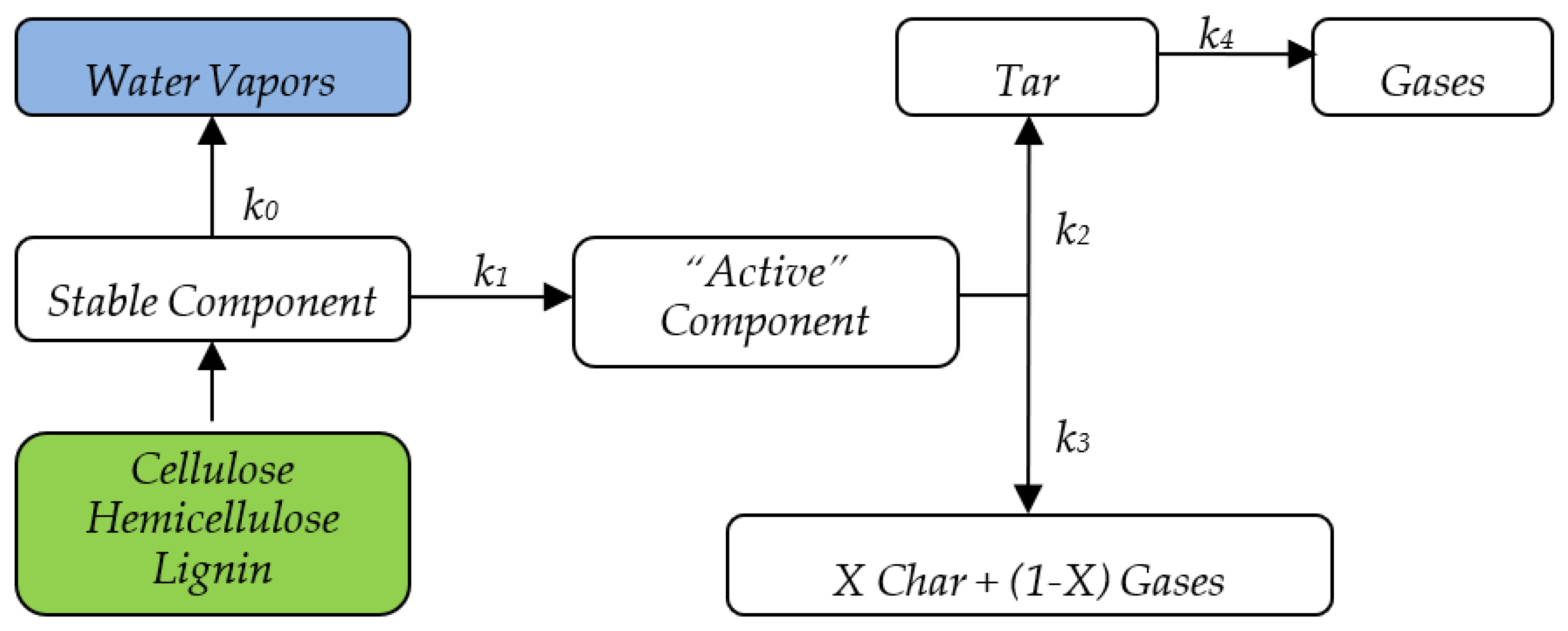