Article

The Effects of the Presence of a Kitchen House on the Wind Flow Surrounding a Low-Rise Building

by
Siti Noratikah Che Deraman
1,†,
Saddam Hussein Abo Sabah
2,†,
Shaharudin Shah Zaini
3,*,
Taksiah A. Majid
3,* and
Amin Al-Fakih
4
1
Department of Civil Engineering, Faculty of Engineering, International Islamic University Malaysia, Jalan Gombak, Selangor 50728, Malaysia
2
Jamilus Research Centre, Faculty of Civil Engineering and Built Environment, Universiti Tun Hussein Onn Malaysia, Batu Pahat, Johor 86400, Malaysia
3
School of Civil Engineering, Engineering Campus, Universiti Sains Malaysia, Nibong Tebal, Penang 14300, Malaysia
4
Department of Civil and Environmental Engineering, Universiti Teknologi PETRONAS (UTP), Bandar Seri Iskandar, Perak 32610, Malaysia
*
Authors to whom correspondence should be addressed.
These authors contributed equally to this work.
Energies 2020, 13(23), 6243; https://doi.org/10.3390/en13236243
Submission received: 7 October 2020 / Revised: 1 November 2020 / Accepted: 21 November 2020 / Published: 26 November 2020
(This article belongs to the Section A3: Wind, Wave and Tidal Energy)

Abstract

:
Most Malaysian rural houses are categorized as non-engineered buildings and vulnerable to damage during events such as windstorms due to the fact that these houses lack engineering considerations. These houses are characterized by having an attached kitchen house, and many of these houses were previously damaged by thunderstorms. The current research investigated the air flow characteristics changes surrounding these houses as a result of the presence of the kitchen. The roof pitch, position, gap height, and overhang were investigated using computational fluid dynamics (CFD) simulations. The results showed that the kitchen position at the center resulted in a slight increase in the suction on the ridge of the roof; however, it significantly altered the flow pattern in the windward and leeward directions. The results also showed that the roof overhang, roof pitch, and kitchen position contributed severely to the damage of the rural house. Moreover, the highest suction occurred at the roof ridge when the kitchen was located at the center of the rural house (Cp = −2.28). Therefore, the authors believe that it is more advantageous to have a kitchen connected to the core as it reduces the pressure on the roof of the core during thunderstorm events.

1. Introduction

Natural events such as hurricanes (tropical cyclones), tornadoes, thunderstorm, downburst, monsoon, and gale are always the main causes of extreme winds [1,2,3,4]. According to Aly [4], it is the wind velocity and the structure properties that influence the behavior of any structure during a wind event.
Tropical cyclones occur in the coastal regions of the tropics and have the tendency to travel for hundreds of kilometers in land. Aly [4] stated that tropical cyclones are the most destructive and powerful storm systems on the face of the earth mentioning the catastrophe caused by hurricane Katrina in 2005, which caused property damage worth more than $75 billion. Fisk [5] concluded that it is most likely that tropical cyclones are going to increase towards the end of the 21st century as this trend has been increasing over the past 20 years. Thus, cyclones have the potential to uproot buildings, trees, and rooftops and cause casualties.
Many researchers such as Xing et al. [6], Irtaza et al. [7], Ozmen et al. [8], and Tominaga et al. [9] have studied the flow characteristics around low-rise buildings. Irtaza et al. [7] described the effects of several factors such as overhang, roof pitch, roof geometry, and surroundings interference on the air flow around low-rise buildings as complicated.
The geometry of the roof plays an important role in the wind load exerted on a structure. Meecham et al. [10] investigated the magnitude and distribution of the exerted wind pressure on both hip and gable roofs using the wind tunnel to measure the fluctuating pressure on the surfaces of the two roofs. The results showed that the distributed pressure on the gable roof was two times higher than the pressure on the gable roof due to the different shapes of the roofs. Ahmad and Kumar [11] tested a Texas Tech University building model under atmospheric boundary layer conditions with various overhang ratios. They concluded that the overhang and aspect ratios of the hip roofs greatly influenced the pressure magnitude and distribution.
The roof pitch is another factor that affects the wind flow surrounding a low-rise building [9,12]; though the exact pitch angle is still a matter of disagreement. Ahmad and Kumar [12] and Xu and Reardon [13] experimentally studied the effect of roof pitch on the pressure distribution of hip roofs for various roof pitches varied between 10 and 40° via the wind tunnel test. The results showed that the 30° roof pitch produced the worst peak suctions. Tominaga et al. [9], Takano and Moonen [14], and Tsuchiya et al. [15] concluded that the flow distribution around a low-rise building is critically influenced by the 20° pitch angle. In addition, Holmes [16] reported that the roof pitch has a significant effect on the roof pressures, especially when the wind is perpendicular to the ridge.
The surroundings such as structures, trees, walls, etc., also affect the air flow around buildings. Generally, low-rise buildings in urban or rural areas are surrounded by various obstructions. Buildings in urban areas are surrounded by neighboring houses and other structures while buildings in the rural area are surrounded by trees. Surry and Lin [17] suggested that the presence of these obstructions reduces the suctions on the roof. Chang and Meroney [18] pointed out that the shielding effects mainly rely on the ratio of spacing distance to building height and the number of upstream buildings.
Due to the location of Malaysia, it is extremely vulnerable to tropical cyclones. Wan Chik et al. [19] reported that several locations all over Malaysia were severely struck by windstorms between 2000 and 2012. According to Bachok et al. [20], these events occurred in a short-time life cycle, typically less than 30 min, and struck the rural areas in terrain Category 1 as classified by the Malaysian Standard (MS 1553:2002) [21]. Generally, this type of terrain is covered with grass and agricultural lands such as the paddy field [19].
Figure 1 depicts some of the rural houses, which were damaged during a windstorm event in Kepala Batas, Penang.
The roofs of rural houses in Malaysia are basically designed and built based on the environmental characteristics of the region, nature, and climatic factors [22,23,24,25]. The construction is solely initiated by the owner who brings a local carpenter without following any proper design or code of practice [26,27]. Therefore, almost all the rural houses in Malaysia are not professionally designed (non-engineered) and are built using readily available local materials matching the local climatic and environmental conditions. Wan Chik e al. [19] reported that most of Malaysian rural low-rise buildings are built of wood and that exposes them to great damage during a wind event. The roof is the weakest link in the structural system of these rural houses due to the weakness of the connections and roofing materials [19]; thus, they are more vulnerable to damage. The damage mechanism of the roof system of rural low-rise buildings in Malaysia were studied by Majid et al. [28]. According to Majid et al. [28], the damage is attributed to the high uplift pressure developed in the house roof.
The typical features of a Malaysian rural house consist of a kitchen house with an overhang roof as shown in Figure 2. Majid et al. [28] reported that such houses get damaged during thunderstorms, especially with the increase of thunderstorms events lately in Malaysia [28]. Several studies were carried out to determine the air flow characteristics of low-rise building using computer simulation or wind tunnel test facilities. The effects of balconies on the airflow of single low-rise buildings via computational fluid dynamics (CFD) were investigated by Ai et al. [29]. The numerical results showed that the addition of balconies increased the mass flow rate and reduced the average velocity in most rooms. Ozmen et al. [8] also studied experimentally and numerically the flow characteristics over the low-rise building models with gabled roofs of different pitch angles and concluded that the mean velocity and turbulence kinetic energy are influenced by the roof pitch. Kumar [30] stated that most of the wind damage he noticed during his study on low building roofs was on the building envelope. Ginger and Letchford [31] performed point and area-averaged pressure measurements for edge regions on a low-rise building roof in a wind tunnel. It was found that fluctuating pressures were measured within regions of flow separation on the roofs of low-rise building. Alemu et al. [32] and Pietrzyk and Hagentoft [33] both developed models to integrate airflow components into single low rise buildings.
As aforementioned, several studies have investigated the air flow characteristics of high-rise and low-rise building using computer simulation or wind tunnel test facilities; however, they focused on the direct air flow characteristics with 0 degrees of a single structure core house without any extensions because most of the data collection from the site were perpendicular to the kitchen house. In other words, the wind flow pattern of rural low-rise buildings when an extension (kitchen) is added has not been investigated, and the effect of overhang and gap formation between the core and kitchen house is not fully understood. Thus, the main objective of this study is to numerically explore the effect of a kitchen addition on the wind flow surrounding a typical rural house in Malaysia.

2. Research Methodology

This research was conducted in different stages as will be explained in this section.

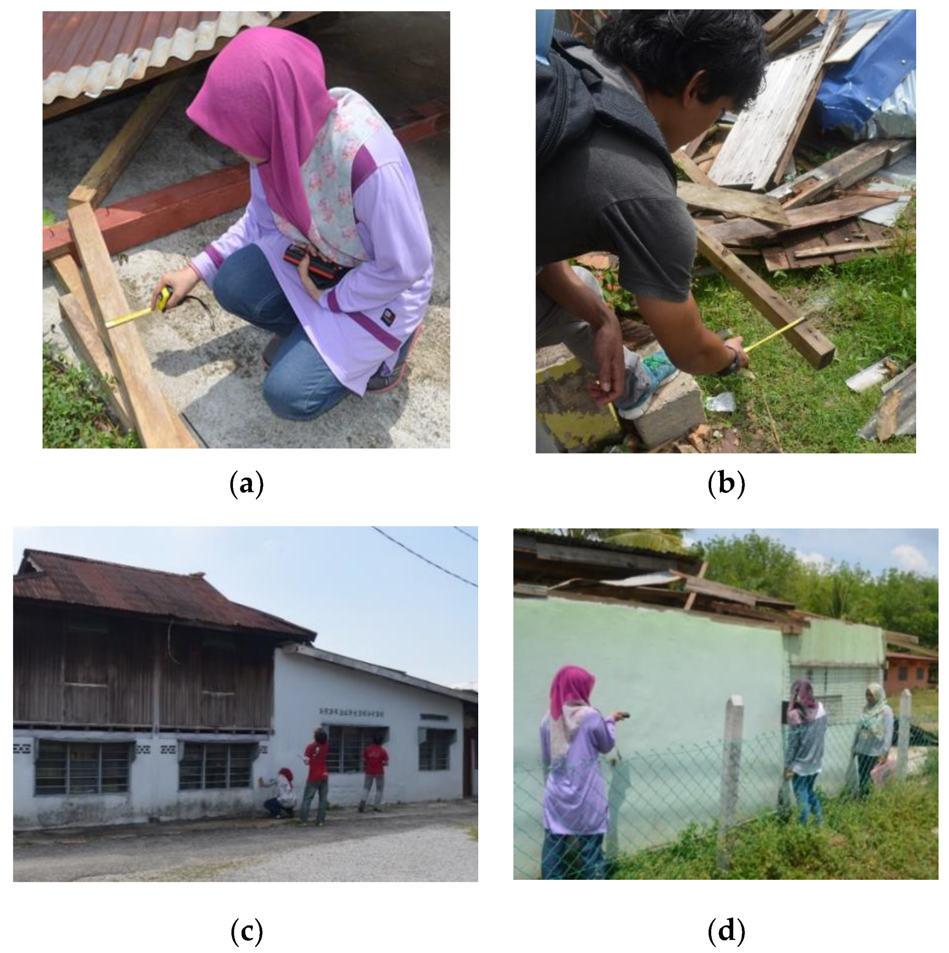
2.1. Post Windstorm Site-Survey

According to Khanduri and Morrow [34], in order to evaluate the vulnerability of buildings in the absence of detailed data, one or both of the following two methods can be employed: applying engineering principles and judgment or observations of post-event damage surveys. In the current study, the observation of post windstorm site-survey was adopted. The survey was carried out to obtain useful information on the building damage and the dimension of the rural house. Such information was extremely essential for the development of the studied house computational model. The survey was aimed to cover only the Northern Region of Peninsula Malaysia because this region was shown to be the most affected by the windstorm event [19]. The data was collected over a period of 20 months, and a total of 35 houses that underwent significant damage to the claddings of the roof, walls, and trusses were taken into consideration in this survey. Different activities were carried out during the post windstorm site-survey such as site visualization, site assessment, and interview sessions with the houses’ owner and the villagers.
The site assessment measured the dimension of the structural elements of the affected houses using a measuring tape and a handheld digital laser distance meter, which can measure a distance up to 100 m in both the horizontal and vertical direction. The measurement of the structural elements included the dimension of purlins, rafters, fasteners’ size, spacings of purlin-rafter, spacing of purlins, and spacing of rafters. In addition, the dimension of the house including length, width, height, roof overhang, and gap height were also measured. Figure 3 shows some of the measurement taken at the site. Finally, the rural house model dimensions were derived using a normalization approach based on the dimensions of rural houses in the Northern Region of Peninsula Malaysia.
The survey showed a specific feature of a rural house that has a kitchen house and a core. It was noticed that there was a gap between the ridge of the kitchen house roof and the leading edge of the core house roof. This gap has the possibility to interfere with the flow characteristic compared to a single core house structure. Thus, the dimension of the gap was taken as one of the parameters in the current study and termed as the “gap height”. Figure 4 shows the cross-section of a rural house depicting the location of the roof pitch, roof overhang, and gap height.

2.2. Numerical Modeling

In this study, the computational fluid dynamic (CFD) simulation consisted of two stages: preprocessing and post-processing employing commercial software GAMBIT 2.4.6, ANSYS Fluent 14.0, and Tecplot 360 freeware.
Moreover, the grid sensitivity analysis was conducted for three different grid schemes namely coarse, medium and fine grids based on the information gained from the post windstorm site survey. The validation of the results of the current study was based on the wind tunnel test (WTT) data of Tominaga et al. [35].

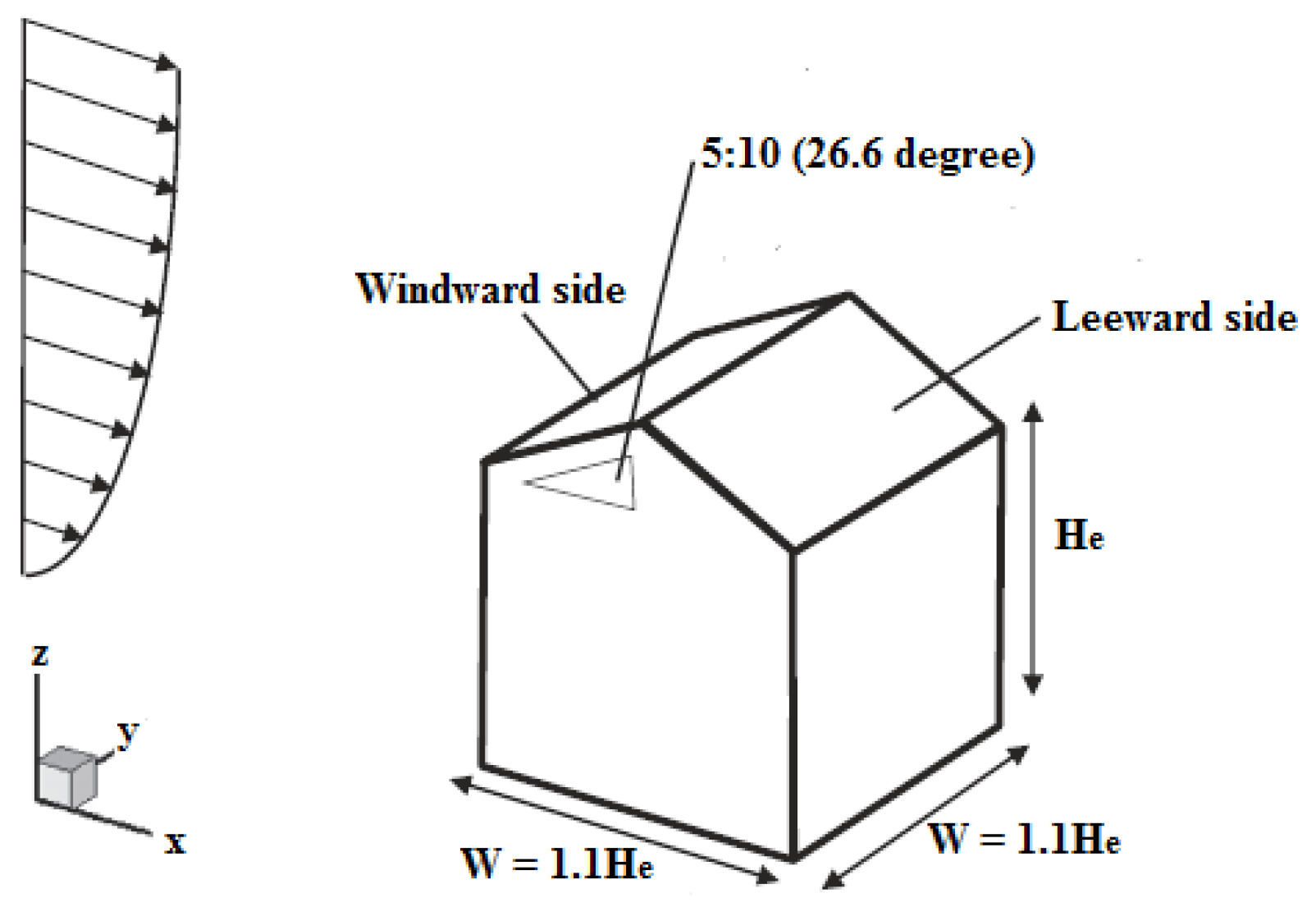
2.3. Validation Model

The validation in this study was based on the wind tunnel test (WTT) and CFD simulation results Tominaga et al. [9] due to the following reasons:
(i)
Tominaga et al. [9] conducted both experiments and CFD.
(ii)
Their isolated low-rise model has strong resemblance of a Malaysian rural house.
(iii)
They conducted their CFD work using the ANSYS Fluent software package, which was used in the current study.
The model used for the validation was an isolated gable-roof building with 1:30 scale following Tominaga et al. [9] with a roof pitch of 26.6°. They based the width and length of the model on the height of the building (He), which was 200 mm. The dimensions of the building model are shown in Figure 5.
In this study, the validation model was developed in a similar manner as the main house model, which will be explained in the following sections using the GAMBIT Graphical User Interface (GUI). The pressure coefficient (CP) results were compared with the CP results of Tominaga et al. [9]. The statistical analysis was performed using the ANOVA test with the aid of SPSS software and error measures.

2.4. Numerical Methods for the House Model

2.4.1. Preprocessing for the House Model

The geometric models for the house were developed based on the geometry of the rural houses in the Northern Region of Peninsula Malaysia. The heights of core house (HC) and kitchen house (HK) were 4 m and 2 m, respectively. The model was perpendicular to the flow within the surface boundary layer. The length, width, and height of the house model were set to be within the ratio of 3:2:1 using the normalizing method as suggested by Zaini et al. [36]. The models were constructed with different parameters of the core and kitchen as summarized in Table 1.
By considering all the variables, a total of 48 different models were generated and analyzed. Figure 6 depicts the used schematic view of the building model.
The model was developed by creating the vertices, straight lines, surfaces and volumes via GAMBIT GUI. After completing the model, the computational domain was formed by creating several volumes using GAMBIT as shown in Figure 7a. Six boundary conditions (Figure 7b) were implemented on the surface of the domain including the surface of the rural house as done by Tominaga et al. [9]. The outlet boundary of the model was set to be 16 H C (minimum 15 H C ), lateral boundary 8 H C (minimum 5 H C ) while the vertical domain and the inlet boundary were set as 9 H C and 6 H C .
A turbulent flow was generated for the model at the inlet boundary condition, and the vertical wind profile was set as the velocity inlet using the power law equation:
V z =   V z r e f ( z z r e f ) α
where V z is the wind velocity at height z, V z r e f is the wind velocity at reference height, z is the height above the ground, z r e f is the reference height (building height), and α is the power-law exponent based on terrain roughness taken as 1/7. For the inlet boundary condition, the wind velocity was calculated following the recommendation of Zhang [37] as follows:
u = u κ l n ( z r e f z 0 )
where u is the wind velocity (m/s), u is the friction velocity (m/s), κ is the Von Karman constant equals to 0.04, and z 0 is the terrain roughness length (m) taken as 0.035 m.
The turbulent kinetic energy was obtained as suggested by Richard and Hoxey [38] and Zhang [37]:
k = u 2 C μ
where k is the turbulent kinetic energy (m2/s2) and C μ is the Kolmogorov constant with the value of 0.09. The turbulence model used in this study was RNG k-ε.
Table 2 presents the air properties for the turbulence flow used in this study.
Figure 8 illustrates the five zones (A to) that were considered to obtain the height of the first cell (2 z p ), where the center must be bigger than the roughness height (KS) as recommended by Zhang [37].

2.4.2. Post-Processing for the House Model

This was the last step in the CFD simulation where the contour, CP values and streamlines were analyzed. Equation (4) was used to calculate the CP value.
C P = ( P S   P r e f ) 0.5 ρ U H e 2
where P S is the static pressure at the middle of wall surfaces, P r e f is the reference pressure, which is at the reference height (the building height), ρ is the air density, and V H e is the velocity at the building height.
In addition, the results of the contour and streamlines were presented using Tecplot 360 EX 2014 software. Upon obtaining the CP values, the percentage difference at each zone was calculated.
The pressure coefficient at the roof overhang was assigned at different locations. The locations and numbers of the cut sections were set differently for overhang lengths of 0.5 m, 0.75 m, and 1.0 m. These cut sections were important to obtain the precise CP values on the overhang. This study also monitored the net pressure at the overhang roof. The net pressure is defined as the total combination of pressure acting on the roof overhang.

3. Experimental Results and Discussions

3.1. Validation Model

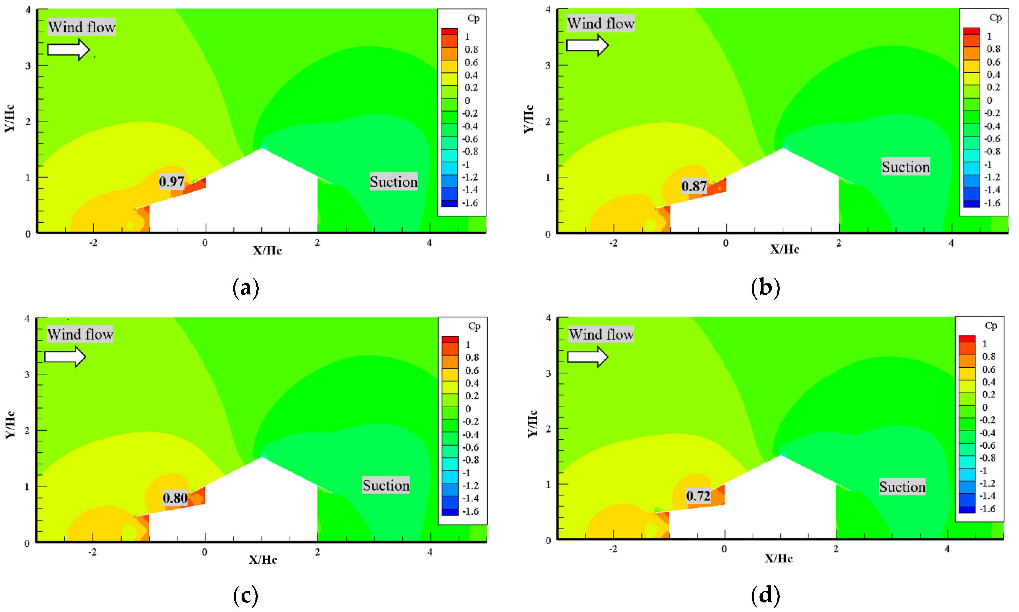
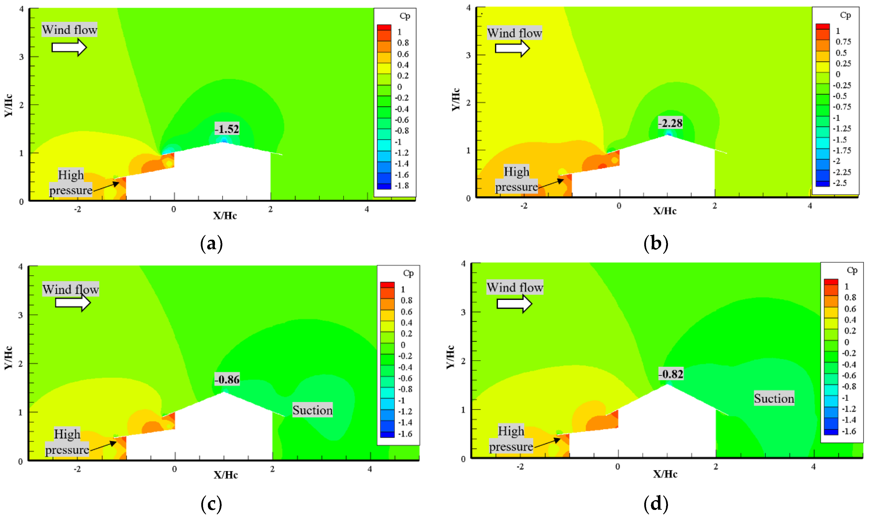
3.1.1. Comparison of Pressure Coefficient

Figure 9 shows that the current study distribution of CP matches those of Tominaga et al. [9] at all zones. It is noticed that the windward wall (Zone A) had the highest-pressure coefficient, especially as it reached Zone B. A sudden drop was experienced in Zone B causing the values of CP to become negative. The CP values then increased and became positive; however, they started to move into negative as they reached the roof apex. In Zones C and D, the pressure then continued to be negative.
The slight variations observed in the results can be associated to the total number of meshed elements used in this study, which were more than those used in the CFD of Tominaga et al. [9].

3.1.2. Comparison of Pressure Coefficient

ANOVA test was conducted to define the similarity of the mean CP between the two studies. In addition, for each case, three error types were measured to obtain the lowest error. These errors were the mean absolute error (MAE), the root mean square error (RMSE), and the normalized absolute error (NAE).
The Games–Howell method was performed on a one-way ANOVA to determine the difference between all unique pairwise comparisons as presented in Table 3. It is obvious that the difference for all cases was insignificant, and the p-values were more than 0.05.
Table 4 summarizes the MAE, the NAE, and the RMSE. For MAE and RMSE, the results show that the smallest errors were seen between this study and WTT. However, the smallest NAE error was experienced between WTT and CFD.
Thus, the overall validation results proved that the outcome of the current study was nearly similar to the numerical and experimental results of Tominaga et al. [9].

3.2. Numerical Simulation of the Rural House Using CFD

3.2.1. Grid Sensitivity Analysis

Prior to the actual simulation, a grid sensitivity analysis (GSA) was performed in order to determine the most suitable meshing scheme [9] that enhances the accuracy and computational time of the numerical results. The analysis was carried out based on three meshes: coarse (2,837,900 cells), medium (4,968,000), and fine (8,154,800 cells) using a structured hexahedral element type. The average y+ values over the windward and the leeward roofs were in the range of 300–1000 for the coarse mesh, and 0–10 for the fine mesh. The medium mesh gave the best range of y+ values compared to those of the coarse and fine meshes; thus, it was adopted in this study. The computational grid consisted of 4,968,000 cells for all models, and the computational time was around 13 h.

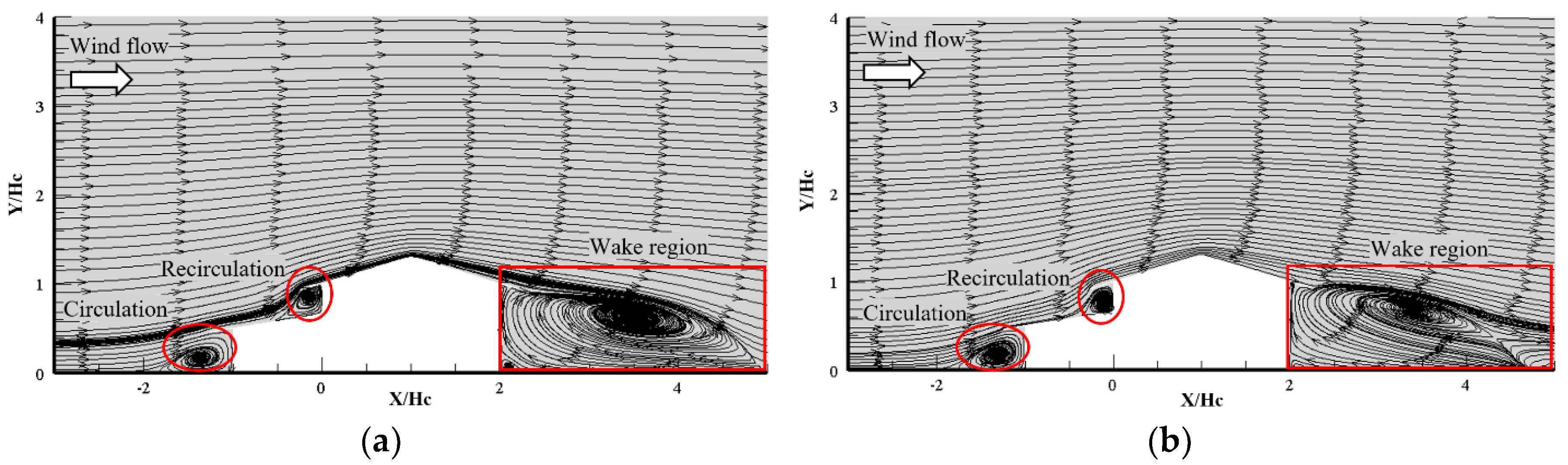
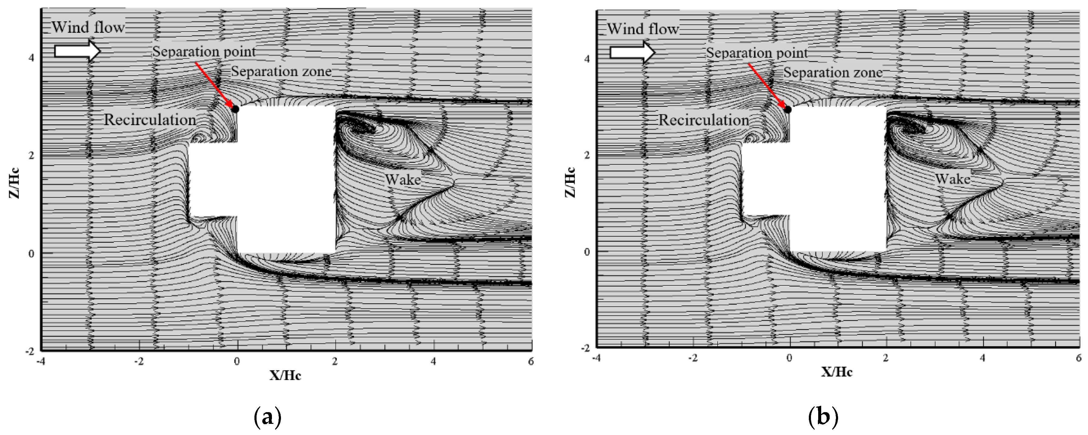
3.2.2. Rural House with and without Kitchen House

This section compares the changes in the airflow properties between models with (kitchen house) and without (core house) a kitchen. The discussion focuses on the general pattern of the streamlines and pressure contours along the transverse profile of the models with roof pitches of 12°, 17°, 22°, and 27°, roof overhang of 0.5 m, and gap height of 0.5 m.
Figure 10 shows the pressure coefficient distribution contours along the transverse profile for the two models. The positive pressure developed on the windward side and caused a high pressure in the wall frontage while the negative pressure developed on the windward wall frontage of the kitchen house. The CP pattern was almost identical for all models with the same roof pitch. Hence, a large upward lift force developed on the underside of the overhang due to the stagnation point generated beneath the overhang. In addition, the kitchen house experienced positive pressure underneath the kitchen and core overhangs. With the wind progression along the roof surface, the suction developed on the upper side of the overhang at the windward side for the core house. At the ridge of the roof, the suction developed on both the roof and downwind slope of the roof.
From the pressure coefficient contours, it is clear that the area of the high positive pressure of the kitchen house model was larger than that of the core house. This is due to the direct impingement of the flow onto the kitchen and the facade behind it that yielded a large stagnation area. In other words, the kitchen acted as a compartment with a nearly constant area. Thus, it can be concluded that the kitchen resulted in high CP values at the windward side.
According to Ozmen et al. [8], the streamline patterns can explain the behavior of the airflow around the rural house. The streamlines for the two models obtained from the CFD analysis are depicted in Figure 11. Larger eddies were formed in front of the core house compared with the kitchen house for the same roof pitch. This effect is due to the large surface area of the wall exposed to the wind flow, which affected the stagnation area. It is worth mentioning that other eddies circulated at the gap height of the kitchen house.
The air pressure on the windward wall was higher than the ambient pressure. The pressure fluctuations on the windward wall were due to the turbulence carried in the approaching flow. However, on the windward surface, the streamlines were only diverted under the kitchen house overhang. For the kitchen house, two stagnation points were developed compared to only one for the core house.
In the roof and near the side walls (the two walls parallel to wind), the air movements were highly turbulent causing a backflow near the surface. The strongest turbulence was generated at the sides of the side wall of the kitchen house resulting in the fluctuation of the negative pressure (suction) due to the separation point at the sharp edge of the kitchen house.
Furthermore, the kitchen presence blocked the wind flow at the windward side. In addition, the kitchen induced the multitude of flow separation and recirculation areas. Montazeri and Blocken [39] stated that the presence of balconies blocks the wind flow at the windward side of the building. Thus, in this study, the presence of the kitchen drastically changed the flow pattern and the overall pressure distribution on the facade.
The wake region behind the roof of the kitchen house was larger than that of the core house creating different flow patterns. In addition, the center of the recirculation eddies behind the roof moved away from the house for the kitchen house making the reattachment length of the eddies become larger. For the core house, it is clear that the recirculation region behind the house became larger with the increase of the roof pitch.

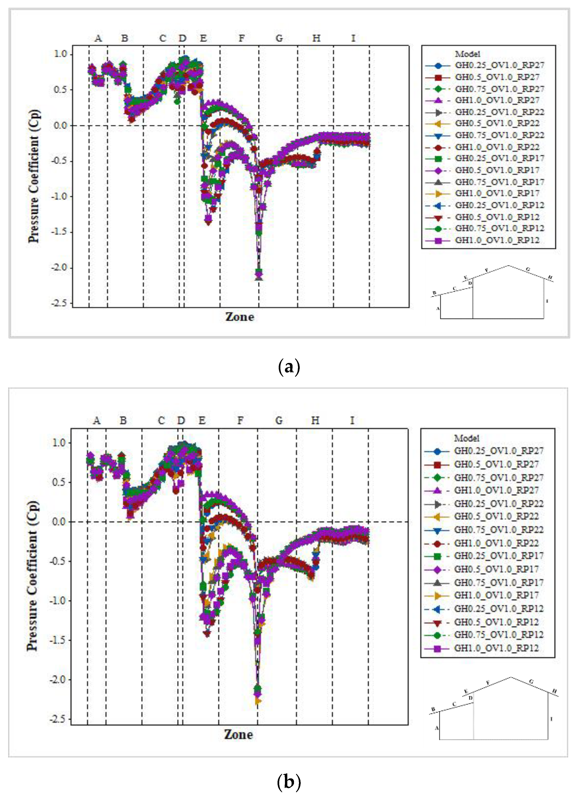
3.3. Factors Affecting the Wind Flow Around a Rural House

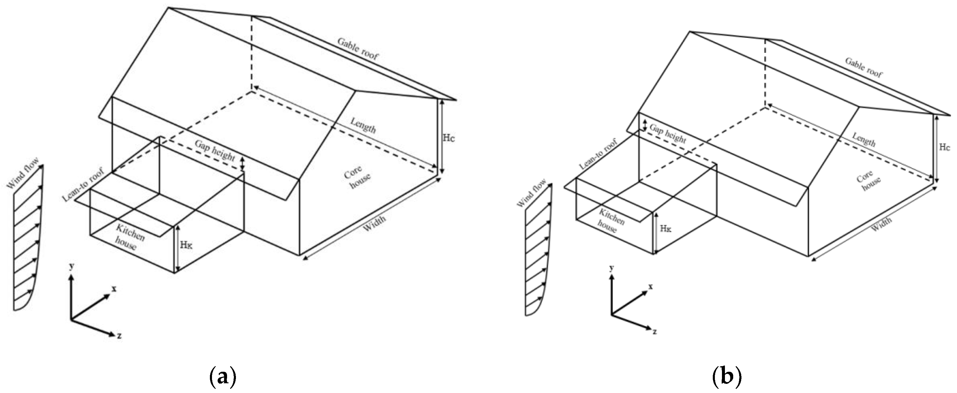
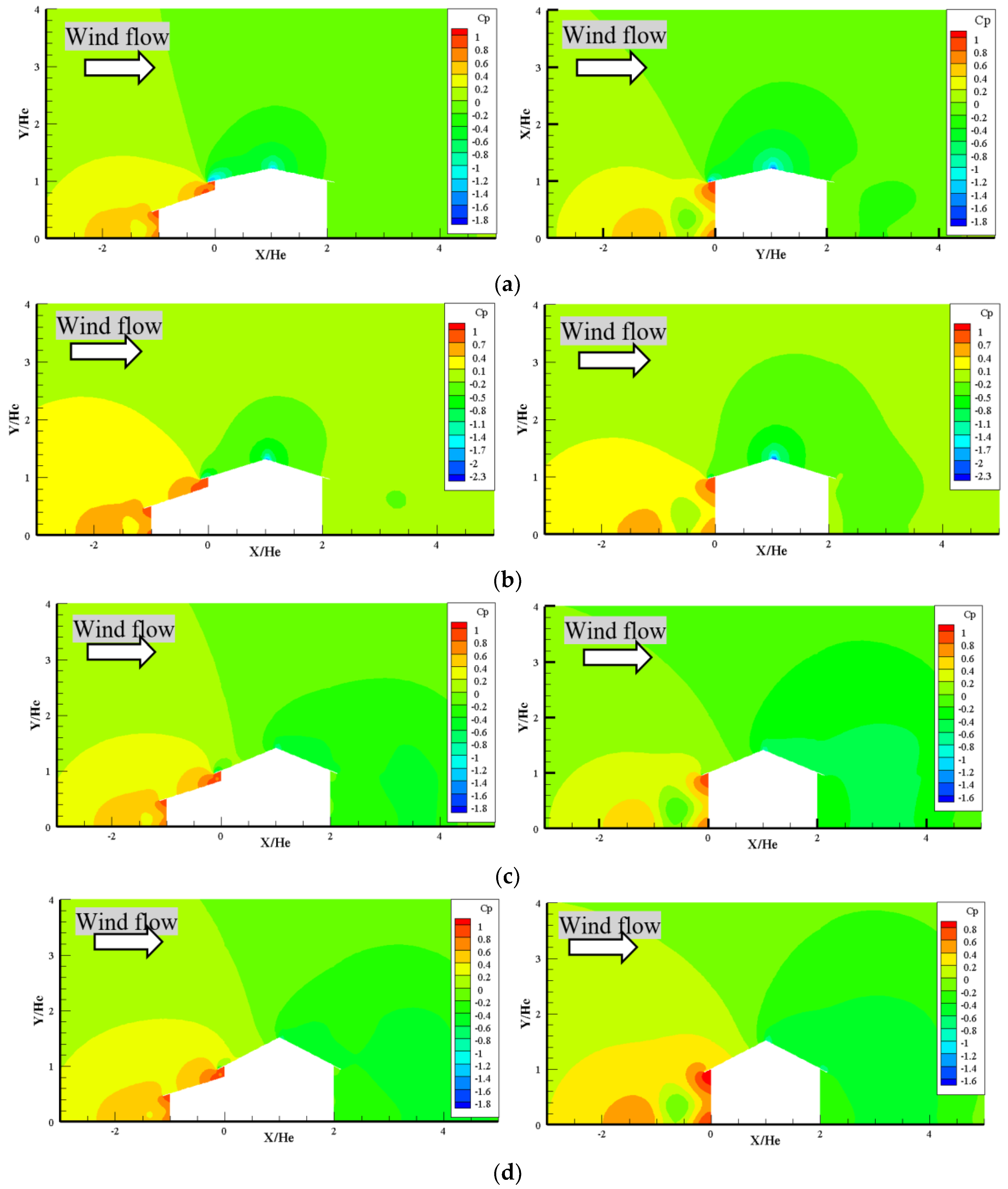
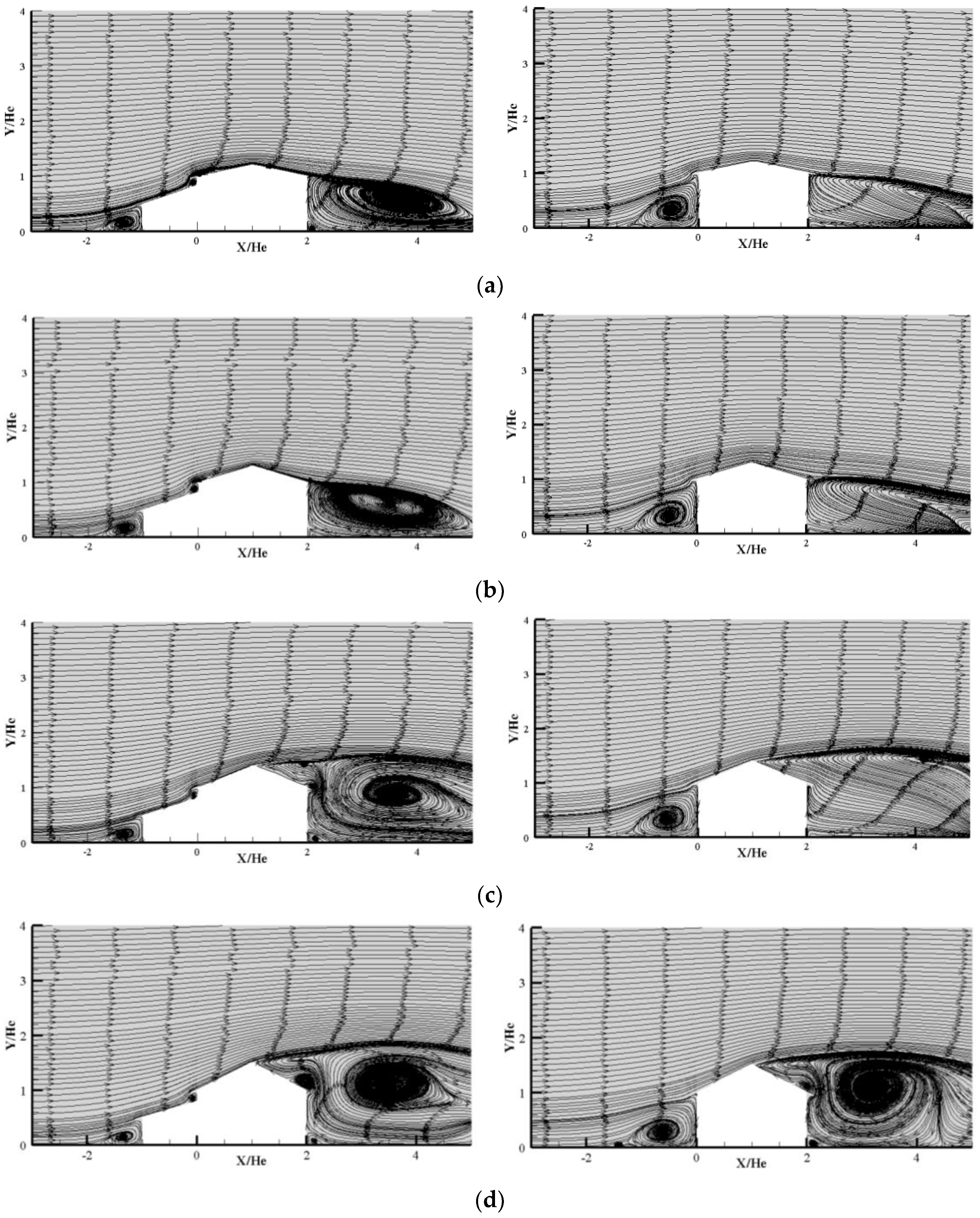
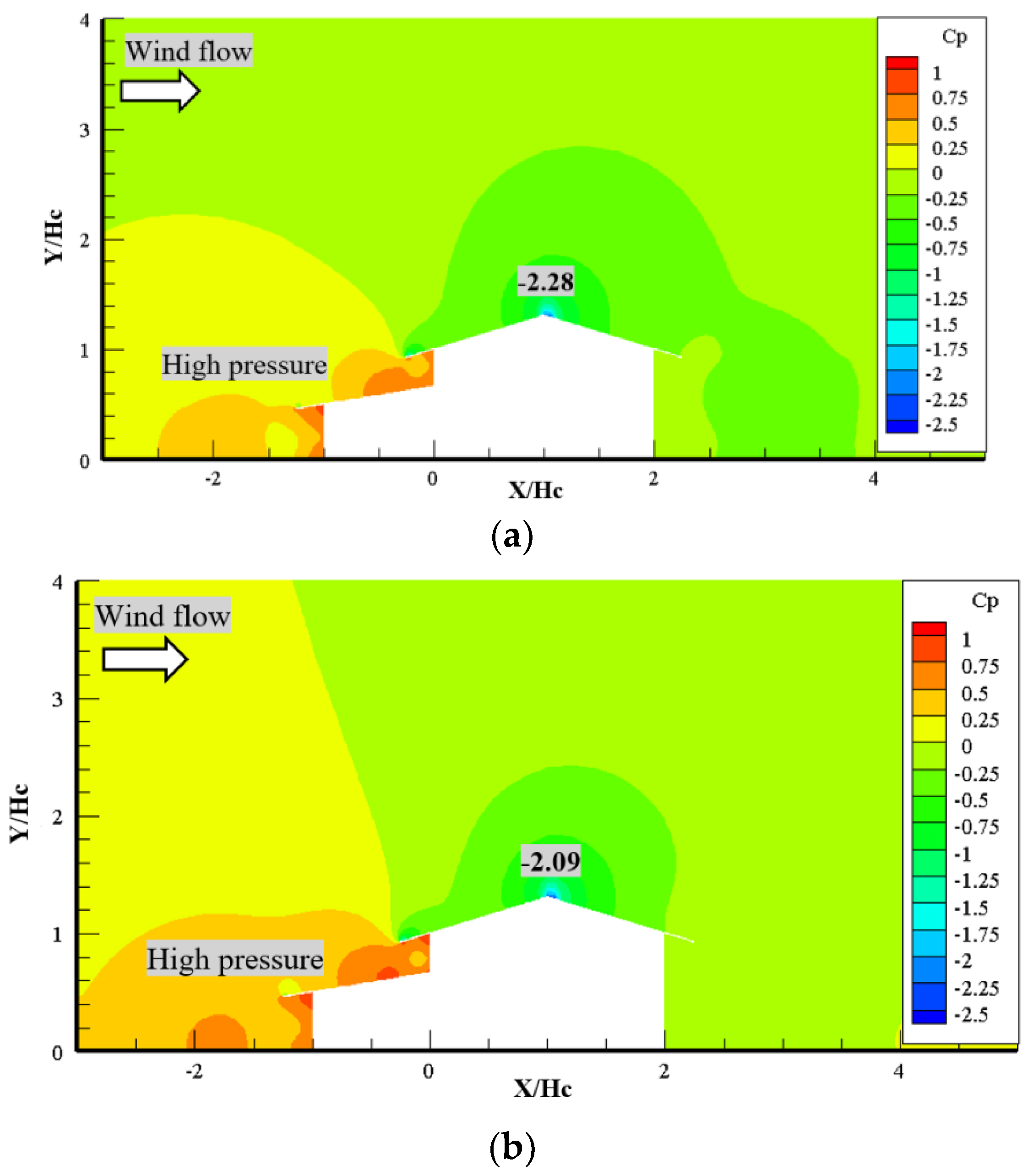
3.3.1. Kitchen Position
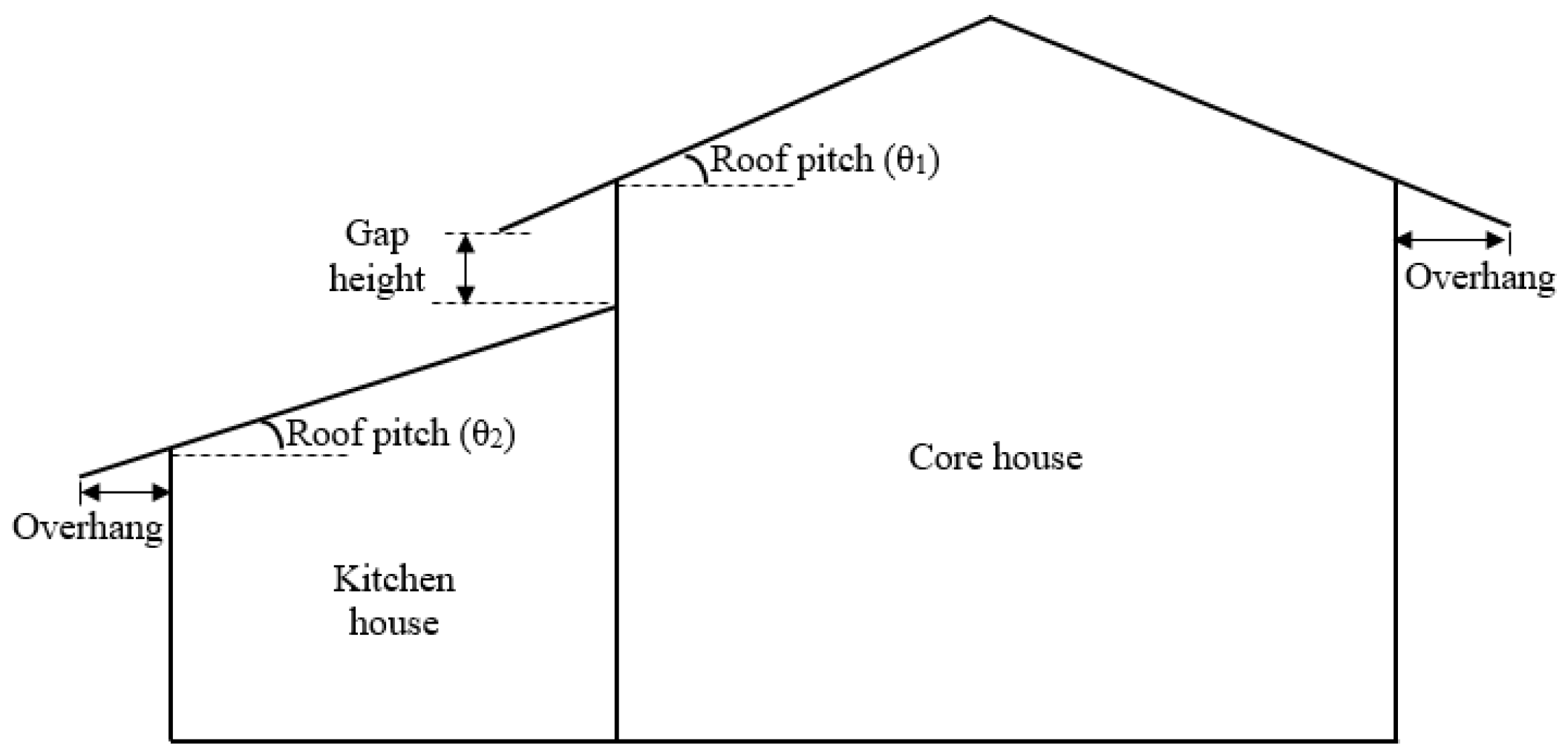
Figure 12 depicts the pressure distribution of the kitchen model when the kitchen is located at the edge and center of the core house for different gap heights. For both positions, the CP started with positive values in Zone A. The positive pressure slightly dropped at the middle of the wall and increased as it approached the upper side of the kitchen house roof. There was a sudden drop on the upper side of Zone B, and the minimum values were close to the edge of the overhang roof.
In Zone C, the CP gradually increased, and the maximum pressure was observed in Zone D. The magnitudes of the positive CP seem to be dependent on the gap height; the higher the gap height, the lower the CP. The positive CP extended to the lower side of the overhang roof of the core in Zone E. Then, a rapid drop was observed on the upper side of Zone E (second pressure drop) transforming the CP values into negative. The maximum suction was localized close to the edge of the overhang roof of the core. The negative CP reduced when approaching the upwind roof of Zone F. However, some models clearly exhibited positive CP, especially for models with roof pitch 22° and 27°.
As the air flow approached the ridge of the roof, the third pressure drop occurred. At this location, all models exhibited the highest suction at roof pitch 17°. The suction reduced again as the air flow passed through the ridge in Zone G and H. The suction became constant in Zone I.
Figure 13 shows that the positive pressure developed at the windward side and upwind slope of the kitchen while the negative pressure (suction) developed at the edge of the overhang. The edge of the overhang became as the separation point and led to the formation of the separation zones along the roof. The separation zones mainly involved the windward portion of the roof. As the wind moved to the upwind slope of the core, the positive pressure changed to negative. The pressure then started to decrease and reached a minimum value at the roof ridge. As the wind approached the downwind slope, the negative pressure developed at the leeward side as well.
The model with the kitchen located at the center underwent higher suction at the leeward side compared to that of the one with the edged kitchen due to the stagnation of eddies at the central part after passing over the house. However, a high positive pressure developed at the windward side of the edged-kitchen model.
Table 5 presents the percentage differences of CP for both kitchen positions at five critical locations (Zone B, Zone D, Zone E, Zone F, and roof ridge). The CP at each zone for the model with the kitchen at the center was set as a reference. The percentage difference in Zone B was significant for both models (340.0%). As the overhang length increased to 0.75 m and 1.0 m, it decreased to 118.0% and 9.0%, respectively. In Zone D, the trend continued to decrease for the overhang lengths of 0.5 m and 0.75 m to 8.0% and 20.6%, respectively. However, the percentage difference for the 1.0 m overhang length increased from 9% to 16.7%. In Zone F, the CP values for the kitchen at the center were greater than those of the edged one and the difference varied between 21.2% and 31.6%. It is also noticed that the highest percentage difference in the windward region was observed in Zone B due to the effect of stagnation pressure at two areas in front of the core generating high pressure at the windward side.
The streamlines for both positions are shown in Figure 14 and Figure 15. It is obvious that a stagnation pressure was generated beneath the overhang as the wind flow impinged the house model. The windward wall deflected the wind flow beneath the overhang roof and circulated as highlighted in the red circle. The wind flow then got separated from both the top and bottom edges of the overhang roof causing a turbulent wake on the upwind side of the roof and produced high pressure. The flow separation continued until the streamlines reached the roof ridge. The size of recirculation under the model overhang roof with the kitchen at the edge was thicker (red circle) resulting in a low pressure underneath the overhang. However, the recirculation behind the core shows different patterns for both models as highlighted in the red rectangle. The thickness of the recirculation eddies for the model with a kitchen at the center was thicker. Moreover, the distance of the recirculation for the centered kitchen was closer to the downwind slope.
Figure 15 shows the plan view of the streamlines for both models. The pattern of the streamlines at the windward side and leeward side were clearly influenced by the position of the kitchen. A small recirculation occurred in front of the windward wall of the core at one side while the other side showed that the streamline flowed away before reattaching with the side wall of the model when the kitchen was at the center. As the wind flowed behind the house, the recirculation happened at one side of the core.
For the kitchen at the edge, this position created a larger recirculation region in front of the core windward wall compared to that of the kitchen at the center due to the large area exposed to the wind flow. As the flow approached the edge of the side wall, it got separated from the edge of the side wall and did not attach itself to the side wall for both models. The vortices were spread through the back of the house model. The mixing layer also formed at the house model leeward side and a region of reverse flow occurred behind the house. The same results were observed by Ozmen et al. [8].
The suction occurred at both sides of the kitchen and core side walls. This phenomenon occurred due to the separation point at the sharp edge of the kitchen, which contributed to the separation zone at that area. The reattachment point occurred at 2/3 of the house width, which experienced the suction zone, and this phenomenon is called reattachment. The air movements were highly turbulent near the side walls (the two walls parallel to wind) causing the backflow near the surface, and this zone is called the separation zone. In addition, the flow at the leeward region (the wake) was highly turbulent.

3.3.2. Gap Height

The CP distribution contours along the transverse profile of the model with different gap heights (0.25 m, 0.5 m, and 1.0 m) are depicted in Figure 16. For 0.25 m (Figure 16a), it is seen that the positive CP developed at the windward side and upwind slope of the kitchen while the negative CP (suction) developed at the edge of the overhang of the core. Moreover, a large area of positive CP developed at the windward side, and the highest CP occurred underneath the kitchen overhang roof. As the wind moved to the upwind slope of the core, the positive CP gradually transformed into suction due to the upward deflection of wind by the windward wall. The flow separation did not occur until the streamlines reached the ridge of the roof. A wake region developed at the leeward side causing fluctuations of the negative CP (suction).
As the gap height increased to 0.5 m, the positive CP developed at the windward side, and the upwind slope became smaller. On the contrary, the negative CP (suction) developed at the edge of the core overhang. However, the suction developed at the upper edge of the kitchen overhang for gap heights of 0.75 m and 1.0 m.

3.3.3. Roof Pitch

Figure 17 shows the pressure coefficient (CP) distribution contour along the transverse profile of the model with different roof pitches when the kitchen was at the center and edge of the core, respectively. The gap height and the overhang were fixed at 1.0 m each.
For the 12° roof pitch, the positive CP developed at the windward side and upwind slope of the kitchen. High CP occurred under the roof overhang of both the core and kitchen. A small area of suction developed at the upper side edge of the kitchen roof overhang. As the wind progressed to the upwind slope of the core, the positive CP gradually transformed into suction due to the wind upward deflection by the windward wall. This situation subjected the entire roofs to suction and strong fluctuations of negative CP. The highest suction developed at the edge of the core roof overhang and the roof ridge shown in the blue color. A wake region developed at leeward side.
When the roof pitch increased to 17°, the positive CP also developed at the windward side and upwind slope of the kitchen. A small suction area developed at the upper side edge of the kitchen roof overhang. As the wind progressed to the upwind slope of the core, the positive pressure gradually transformed into suction. This was due to the wind upward deflection of wind by the windward wall causing the entire roof to be surrounded with a flow separation zone. The highest negative pressure developed at the ridge of the roof shown in the blue color. The entire region at the leeward side developed a wake region, which was less turbulent than that of the 12° roof pitch.
In the case of roof pitch 22°, positive CP developed at the windward side and upwind slope of the kitchen. High pressure also occurred under the roof overhang of both the core and kitchen but the area of positive pressure in the windward side was smaller than that of the roof pitch 17°. As the wind flow progressed to the upwind slope of the core, the entire roof was exposed to suction and strong fluctuations of negative pressure. The entire zone of the leeward experienced higher suction than the previous two roof pitches.
Finally, for the roof pitch 27°, the positive pressure area in the windward side became larger due to the roof pitch increase. The suction developed at the upper side of the kitchen roof overhang. The flow separation did not occur until the streamlines reached the ridge of the roof. Therefore, only the leeward half of the roof experienced the flow separation. The area of leeward side experienced the highest suction.

3.3.4. Roof Overhang

The effects of the overhang (0.5 m, 0.75 m, and 1.0 m) on the CP distribution contours when the kitchen was positioned at the core center are illustrated in Figure 18. The gap height and the roof pitch were fixed at 1.0 m and 12°, respectively.
In the case of the 0.5 m roof overhang, the positive CP developed at the windward side and upwind slope of the kitchen. This area was loaded severely due to the wind impingement on the house model causing high pressure under the roof overhang of both the core and kitchen. A small suction area developed at the edge of the upper side of the kitchen overhang roof. With the wind progression to the upwind slope of the core, the positive CP gradually turned into suction. The wind flow also deflected from the windward wall and increased the pressure on the lower eave surface, which reinforced the high negative pressure on the upper eave surface after separation immediately. This situation subjected the whole roof to strong fluctuations of suction. The highest suction developed at the edge of the core overhang and the roof ridge as shown in the blue color. The entire region at the leeward side developed a wake region, and the pressure of air was below the ambient pressure with strong turbulences.
As the overhang length increased to 0.75 m and 1.0 m, the area of positive CP in front of the kitchen was similar to that of the 0.5 m. The significant effect was observed at the windward side, especially under the core overhang. As the blockage area increased, the area of high pressure underneath the core overhang became larger.
Overall, the results proved that the position of the kitchen at the center slightly increased the negative pressure on the ridge of the roof; however, it significantly changed the pattern of the flow in the windward and leeward directions. The results also showed that the roof overhang, roof pitch, and kitchen position contributed severely to the damage of the rural house. Moreover, the highest negative pressure occurred at the roof ridge when the kitchen was located at the center of the rural house (Cp = −2.28). Therefore, the authors believe that it is more advantageous to have a kitchen connected to the core as it reduces the pressure on the roof of the core during thunderstorm events.

4. Conclusions

The post windstorm survey evaluated the house features that affected the wind flow surrounding a typical Malaysian rural house. The validation results were in good agreement with those of Tominaga et al. [9].
The kitchen presence strongly influenced the wind flow surrounding the rural house causing a succession of zones with low and high pressures. The highest negative pressure developed at the ridge when the position of kitchen was at the edge (Cp = −2.09), but more suction was experienced around the house when the kitchen was located at the center of the core (Cp = −2.28). This was due to the symmetric distribution of the pressure.
The results also showed that as the gap height increased, the pressure increased; however, it did not significantly affect the overall wind flow around the house.
The roof pitch significantly influenced the wind flow surrounding the house, in particular at the rear of the house. The highest negative pressure (Cp = −2.28) occurred at the roof ridge with the 17° roof pitch. As the roof pitch got steeper, the wind flow moved away from the downwind slope causing a large wake region behind the house.
Overall, the attachment of the kitchen to the core of a rural low-rise building helped reduce the pressure on the roof of the core during storm events. Hence, this will minimize the damage to the core house.

Author Contributions

The work presented here was carried out through the cooperation of all authors. S.N.C.D., S.H.A.S., S.S.Z., and T.A.M. conducted the research and wrote the paper. They edited the manuscript including the literature review. A.A.-F. helped during the revision stage. All authors have read and agreed to the published version of the manuscript.

Funding

“This research was funded by Universiti Sains Malaysia, grant number 1001/PAWAM/8014023” and “The APC was funded by Universiti Sains Malaysia”.

Acknowledgments

The authors express their gratitude for the financial support of the Research University Grant from Universiti Sains Malaysia. The authors also thank Universiti Tun Hussein Onn Malaysia for the support of a postdoctoral fellowship.

Conflicts of Interest

The authors declare no conflict of interest.

References

  1. Henry, L. Wind Engineering: A Handbook for Structural Engineers; Prentice-Hall: Englewood Cliffs, NJ, USA, 1991. [Google Scholar]
  2. Henderson, D.; Ginger, J. Role of building codes and construction standards in windstorm disaster mitigation. Aust. J. Emerg. Manag. 2008, 23, 40. [Google Scholar]
  3. Xing, F.; Mohotti, D.; Chauhan, K. Experimental and numerical study on mean pressure distributions around an isolated gable roof building with and without openings. Build. Environ. 2018, 132, 30–44. [Google Scholar] [CrossRef]
  4. Aly, A.M. Atmospheric boundary-layer simulation for the built environment: Past, present and future. Build. Environ. 2014, 75, 206–221. [Google Scholar] [CrossRef]
  5. Fisk, W.J. Review of some effects of climate change on indoor environmental quality and health and associated no-regrets mitigation measures. Build. Environ. 2015, 86, 70–80. [Google Scholar] [CrossRef] [Green Version]
  6. Xing, F.; Mohotti, D.; Chauhan, K. Study on localised wind pressure development in gable roof buildings having different roof pitches with experiments, RANS and LES simulation models. Build. Environ. 2018, 143, 240–257. [Google Scholar] [CrossRef]
  7. Irtaza, H.; Javed, M.; Jameel, A. Effect on wind pressures by variation of roof pitch of low-rise hip-roof building. Asian J. Civ. Eng. 2015, 16, 869–889. [Google Scholar]
  8. Ozmen, Y.; Baydar, E.; Van Beeck, J. Wind flow over the low-rise building models with gabled roofs having different pitch angles. Build. Environ. 2016, 95, 63–74. [Google Scholar] [CrossRef]
  9. Tominaga, Y.; Akabayashi, S.-I.; Kitahara, T.; Arinami, Y. Air flow around isolated gable-roof buildings with different roof pitches: Wind tunnel experiments and CFD simulations. Build. Environ. 2015, 84, 204–213. [Google Scholar] [CrossRef]
  10. Meecham, D.; Surry, D.; Davenport, A. The magnitude and distribution of wind-induced pressures on hip and gable roofs. J. Wind Eng. Ind. Aerodyn. 1991, 38, 257–272. [Google Scholar] [CrossRef]
  11. Ahmad, S.; Kumar, K. Effect of geometry on wind pressures on low-rise hip roof buildings. J. Wind Eng. Ind. Aerodyn. 2002, 90, 755–779. [Google Scholar] [CrossRef]
  12. Ahmad, S.; Kumar, K. Wind pressures on low-rise hip roof buildings. Wind Struct. 2002, 5, 493–514. [Google Scholar] [CrossRef]
  13. Xu, Y.; Reardon, G. Variations of wind pressure on hip roofs with roof pitch. J. Wind Eng. Ind. Aerodyn. 1998, 73, 267–284. [Google Scholar] [CrossRef]
  14. Takano, Y.; Moonen, P. On the influence of roof shape on flow and dispersion in an urban street canyon. J. Wind Eng. Ind. Aerodyn. 2013, 123, 107–120. [Google Scholar] [CrossRef]
  15. Tsuchiya, M.; Murakami, S.; Mochida, A.; Kondo, K.; Ishida, Y. Development of a new k− ε model for flow and pressure fields around bluff body. J. Wind Eng. Ind. Aerodyn. 1997, 67, 169–182. [Google Scholar] [CrossRef]
  16. Holmes, J.D. Wind pressures on tropical housing. J. Wind Eng. Ind. Aerodyn. 1994, 53, 105–123. [Google Scholar] [CrossRef]
  17. Surry, D.; Lin, J. The effect of surroundings and roof corner geometric modifications on roof pressures on low-rise buildings. J. Wind Eng. Ind. Aerodyn. 1995, 58, 113–138. [Google Scholar] [CrossRef]
  18. Chang, C.-H.; Meroney, R.N. The effect of surroundings with different separation distances on surface pressures on low-rise buildings. J. Wind Eng. Ind. Aerodyn. 2003, 91, 1039–1050. [Google Scholar] [CrossRef] [Green Version]
  19. Wan Chik, F.; Che Deraman, S.; Noram, I.R.; Muhammad, M.; Majid, T.; Zulkarnain, N. Development of Windstorm Database System for Wind Damages in Malaysia. J. Civ. Eng. Res. 2014, 4, 214–217. [Google Scholar]
  20. Bachok, M.F.; Shamsudin, S.; Abidin, R.Z. Effectiveness of Windstorm-Producing Thunderstorms Early Warning Issues in Peninsular Malaysia. Int. J. Environ. Sci. Dev. 2015, 6, 635. [Google Scholar] [CrossRef] [Green Version]
  21. MS 1553:2002. Malaysia Standard Code of Practise on Wind Loading for Building; Department of Standards Malaysia: Selangor, Malaysia, 2002. [Google Scholar]
  22. GhaffarianHoseini, A.; Berardi, U.; Dahlan, N.D.; GhaffarianHoseini, A. What can we learn from Malay vernacular houses? Sustain. Cities Soc. 2014, 13, 157–170. [Google Scholar] [CrossRef]
  23. Ghaffarianhoseini, A.; Berardi, U.; Ghaffarianhoseini, A. Thermal performance characteristics of unshaded courtyards in hot and humid climates. Build. Environ. 2015, 87, 154–168. [Google Scholar] [CrossRef]
  24. Kubota, T.; Zakaria, M.A.; Abe, S.; Toe, D.H.C. Thermal functions of internal courtyards in traditional Chinese shophouses in the hot-humid climate of Malaysia. Build. Environ. 2017, 112, 115–131. [Google Scholar] [CrossRef]
  25. Kyritsi, E.; Michael, A. An assessment of the impact of natural ventilation strategies and window opening patterns in office buildings in the mediterranean basin. Build. Environ. 2019, 175, 106384. [Google Scholar] [CrossRef]
  26. Roosli, R.; Bakar, A.H.A.; Abas, N.F.; Ismail, M.; Abdullah, S.; Yusuf, M.N. Criteria and determinants for assessing the sustainability of conservation management and process of Malay Vernacular House. Adv. Environ. Biol. 2015, 59–63. [Google Scholar]
  27. Lim, J.Y. The Malay House: Rediscovering Malaysia’s Indigenous Shelter System; Institut Masyarakat: Kuala Lumpur, Malaysia, 1987. [Google Scholar]
  28. Majid, T.; Ramli, N.I.; Ali, M.; Saad, M.S.H. Malaysia Country Report 2012: Wind Related Disaster Risk Reduction and Wind Environmental Issues. In 7th Workshop on Regional Harmonization of Wind Loading and Wind Environmental Specifications in Asia-Pacific Economies; Universiti Malaysia Pahang: Kuantan, Pahang, Malaysia, 2012; pp. 12–13. [Google Scholar]
  29. Ai, Z.; Mak, C.; Niu, J.; Li, Z.; Zhou, Q. The effect of balconies on ventilation performance of low-rise buildings. Indoor Built Environ. 2011, 20, 649–660. [Google Scholar] [CrossRef]
  30. Kumar, K.S.; Stathopoulos, T. Computer Simulation of fluctuating wind pressures on low building roofs. Concordia University. J. Wind Eng. Ind. Aerodyn. 1997, 69, 485–495. [Google Scholar] [CrossRef]
  31. Ginger, J.; Letchford, C. Pressure factors for edge regions on low rise building roofs. J. Wind Eng. Ind. Aerodyn. 1995, 54, 337–344. [Google Scholar] [CrossRef]
  32. Alemu, A.T.; Saman, W.; Belusko, M. A model for integrating passive and low energy airflow components into low rise buildings. Energy Build. 2012, 49, 148–157. [Google Scholar] [CrossRef]
  33. Pietrzyk, K.; Hagentoft, C.-E. Probabilistic analysis of air infiltration in low-rise buildings. Build. Environ. 2008, 43, 537–549. [Google Scholar] [CrossRef]
  34. Khanduri, A.; Morrow, G. Vulnerability of buildings to windstorms and insurance loss estimation. J. Wind Eng. Ind. Aerodyn. 2003, 91, 455–467. [Google Scholar] [CrossRef]
  35. Tominaga, Y.; Stathopoulos, T. Numerical simulation of dispersion around an isolated cubic building: Comparison of various types of k–ɛ models. Atmos. Environ. 2009, 43, 3200–3210. [Google Scholar] [CrossRef]
  36. Zaini, S.S.; Majid, T.A.; Deraman, S.N.C.; Chik, F.A.W.; Muhammad, M.K.A. Post Windstorm Evaluation of Critical Aspects Causing Damage to Rural Houses in the Northern Region of Peninsular Malaysia. In MATEC Web of Conferences, 2017; EDP Sciences: Ulis, France, 2017; p. 03016. [Google Scholar]
  37. Zhang, X. CFD Simulation of Neutral ABL Flows; Risø National Laboratory: Roskilde, Denmark, 2009. [Google Scholar]
  38. Richards, P.; Hoxey, R. Appropriate boundary conditions for computational wind engineering models using the k-ϵ turbulence model. J. Wind Eng. Ind. Aerodyn. 1993, 46, 145–153. [Google Scholar] [CrossRef]
  39. Montazeri, H.; Blocken, B. CFD simulation of wind-induced pressure coefficients on buildings with and without balconies: Validation and sensitivity analysis. Build. Environ. 2013, 60, 137–149. [Google Scholar] [CrossRef]
Figure 1. Tropical cyclones damage in rural areas in Malaysia.
Energies 13 06243 g001
Figure 2. A typical rural house in Malaysia.
Energies 13 06243 g002
Figure 3. Measurements of the (a) roof truss width; (b) roof truss thickness; (c) height of the house; and (d) width of the house.
Energies 13 06243 g003
Figure 4. A typical cross section of a rural house.
Energies 13 06243 g004
Figure 5. A Schematic diagram of the validation model [9].
Energies 13 06243 g005
Figure 6. A diagram of a Malaysian rural house with a kitchen at the (a) center and (b) edge.
Energies 13 06243 g006
Figure 7. (a) Computational domain and (b) boundary conditions of the rural house model.
Energies 13 06243 g007
Figure 8. A diagram of the sections generating the grid at the bottom of the computational domain for each section.
Energies 13 06243 g008
Figure 9. Comparison of pressure coefficients.
Energies 13 06243 g009
Figure 10. The pressure coefficient contours with roof pitch (a) 12°; (b) 17°; (c) 22°; and (d) 27° (note: right side = core house, left side = kitchen house).
Energies 13 06243 g010
Figure 11. The streamline patterns with roof pitch (a) 12°; (b) 17°; (c) 22°; and (d) 27° (note: right side = core house, left side = kitchen house).
Energies 13 06243 g011
Figure 12. Pressure distribution profiles based on the kitchen location: (a) edge and (b) center.
Energies 13 06243 g012
Figure 13. Pressure contours along the transverse profile of the house model with the kitchen at the (a) center and (b) edge.
Energies 13 06243 g013
Figure 14. The streamlines for the model with kitchen at the (a) center and (b) edge.
Energies 13 06243 g014
Figure 15. The streamlines plan view with kitchen at the (a) center and (b) edge.
Energies 13 06243 g015
Figure 16. The pressure coefficient contours along the transverse profile with gap heights of (a) 0.25 m; (b) 0.5 m; (c) 0.75 m; and (d) 1.0 m.
Energies 13 06243 g016
Figure 17. The pressure coefficient contours for model with kitchen at the center with a roof pitch of (a) 12°; (b) 17°; (c) 22°; and (d) 27°.
Energies 13 06243 g017
Figure 18. The pressure coefficient contours with an overhang length of (a) 0.5 m; (b) 0.75 m; and (c) 1.0 m.
Energies 13 06243 g018aEnergies 13 06243 g018b
Table 1. Parameters of the rural house.
ParametersCore HouseKitchen House
House dimension12 m (L) × 8 m (W) × 4 m (HC)6 m (L) × 4 m (W) × 2 m (HK)
Overhang (OV)0.5 m, 0.75 m, 1.0 m0.5 m, 0.75 m, 1.0 m
Gap height (GH)0.25 m, 0.5 m, 0.75 m, 1.0 m-
Roof pitch (RP)12°, 17°, 22°, 27°Varies with gap height
Table 2. Air properties.
ParametersValue
Air density, ρ1.172 kg/m3
Dynamic viscosity, μ1.8628 × 10⁻⁵ kg/m.s
Reference temperature, T28 °C
Wind speed, V26.4 m/s
Table 3. ANOVA test results.
(I) Group(J) GroupMean Difference (I-J)p
Games–HowellCurrent studyWTT [9]
CFD [9]
−0.0938
−0.0246
0.891
0.987
WTT [9]Current study
CFD [9]
0.0692
0.0938
0.891
0.837
CFD [9]Current study
WTT [9]
−0.0246
−0.0938
0.987
0.837
Table 4. Error measures.
WTT [9]–CFD [9]WTT [9]–Current StudyCFD [9]–Current Study
MAE0.1129170.0989840.130353
NAE0.2219490.2336590.307706
RMSE0.1821490.112218 0.154472
Table 5. Percentage difference of pressure coefficients for different kitchen positions.
Overhang Length (m)Percentage Difference CP (%)
Zone B Zone D Zone E Zone F Ridge
Position of Kitchen HousePosition of Kitchen HousePosition of Kitchen HousePosition of Kitchen HousePosition of Kitchen House
CenterEdgeCenterEdgeCenterEdgeCenterEdgeCenterEdge
0.50−340.00−8.00−27.3031.60−9.0
0.750−118.00−20.6043.8025.001.0
1.00−9.0016.707.4021.208.3
Note: A negative value indicates a decrease in the percentage difference.
Publisher’s Note: MDPI stays neutral with regard to jurisdictional claims in published maps and institutional affiliations.

