Article

Nature-Inspired Algorithm Implemented for Stable Radial Basis Function Neural Controller of Electric Drive with Induction Motor

Department of Electrical Machines, Drives and Measurements, Wroclaw University of Science and Technology, Smoluchowskiego 19, 50-372 Wroclaw, Poland
Energies 2020, 13(24), 6541; https://doi.org/10.3390/en13246541
Submission received: 23 October 2020 / Revised: 4 December 2020 / Accepted: 8 December 2020 / Published: 11 December 2020
(This article belongs to the Section A1: Smart Grids and Microgrids)

Abstract

:
The main point of this paper was to perform the design process for and verify the properties of an adaptive neural controller implemented for a real nonlinear object—an electric drive with an Induction Motor (IM). The controller was composed as a parallel combination of the classical Proportional-Integral (PI) structure, and the second part was based on Radial Basis Function Neural Networks (RBFNNs) with the on-line recalculation of the weight layer. The algorithm for the adaptive element of the speed controller contained two parts in parallel. The first of them was dedicated for the main path of the neural network calculations. The second realized the equations of the adaptation law. The stability of the control system was provided according to the Lyapunov theorem. However, one of the main issues described in this work is the optimization of the constant part of the analyzed parallel speed controller. For this purpose, the Grey Wolf Optimizer (GWO) was applied. A deep analysis of the data processing during the calculations of this technique is shown. The implemented controller, based on the theory of neural networks, is an adaptive system that allows precise motor control. It ensures the precise and dynamic response of the electric drive. The theoretical considerations were firstly verified during the simulations. Then, experimental tests were performed (using a dSPACE1103 card and an induction machine with a rated power of 1.1 kW).

1. Introduction

Over the years, induction motors have been the dominant elements of energy conversion systems. The reasons for this are the low costs of the machines, dynamic features and high reliability [1,2,3]. Currently, the parameters of electric machines have significantly improved; this is the result of new technology in material fabrication and the presently popular numerical tools used for the design process. Moreover, cheap programming devices with high computational power are generally available. The above facts and the large number of industrial applications have led to increased requirements for drive systems with induction motors. A significant group of this devices needs precision of work (the dynamic control of speed or position) under disturbances, a simplified design methodology and the reduction of implementation costs [4,5]. However, meeting the above assumptions can be problematic in the real use of electrical machines. The operation of the electrical drive is often realized under the following conditions: the presence of parameter changes, measured disturbances, delays in signal processing, problems with proper identification, etc. The nonlinearity of the object is another factor that impedes the effective control of the drive.
Theoretical considerations in the field of control theory (control methods or observer algorithms) in applications to practical problems are more complicated. This is caused by the nonlinearity of plants. Linear models have significant limitations, resulting from the linear combination of input signals, in the representation of certain features of the analyzed phenomena. In such cases, nonlinear algorithms should be applied. However, there are problems with the complex design of control systems for such electric drives. In addition, there is a need to perform additional tasks related to the identification of nonlinear elements. In addition, attention should be paid to possible changes in nonlinear phenomena during the work of the drive [6,7,8].
Classic control systems based on PI controllers are still very often used in industry. These methods allow the effective control of state variables, and also do not require significant computing power for the microcontrollers [9]. However, when disturbances occur, the convergence between the reference signal and the output variable can decrease significantly [10]. However, some of the above-mentioned expectations can be obtained through the use of control algorithms based on the theory of artificial intelligence. After careful analysis of the available publications, two dominant trends can be observed. The first group is focused on fuzzy logic. The most characteristic element of these algorithms is the fuzzification of the processed data and operation according to a defined base of rules [11]. These solutions are treated as robust control methods. However, the seemingly simplified design process (rule base) is associated with the troublesome determination of the coefficients used in the controllers. This is problematic, because it is difficult to find the equations describing these parameters. Stability analysis is also a complicated process. The second group, among modern algorithms, is based on neural networks. These models can be successfully tuned, in the training process, to the task. However, the design problems concern the selection of the structure and the development of the training data (which describe the problem with sufficient accuracy) [12].
Due to the above-mentioned characteristic properties of plants and control methods, the application of adaptive neural control seems to be appropriate. Tuning the parameters of the neural model implemented in the speed control loop, aimed at reducing the speed control error of the drive, generates a command signal. The neural network has variable parameters (weights) adjusted during training (the adaptation process). This means that the controller can be modified in response to changes in the object. With such assumptions (of the analyzed control structure), fast responses to disturbances are possible. Moreover, the direct identification of the object is not necessary, which is very beneficial in industrial conditions [13,14,15,16,17,18,19,20,21].
The applications of adaptive neural controllers are often described in journals focused on electric drives and artificial intelligence. These issues are related to the development of theoretical rules, and a separate part presents hardware implementations. Various controller topologies (based on many types of neural networks, e.g., feed-forward networks or those containing internal feedback—recurrent networks) have been analyzed [22,23,24]. For adaptive controllers based on neural networks, algorithms with gradient calculations are most often used [25]. The hardware part of the setups can be classified according to the following (dominant) issues: the applications for miscellaneous types of electrical machines [26,27], the purpose of the application (e.g., in robotics) [28,29,30], problems related to the mechanical part (nonlinearities—backlash or shaft elasticity) [31], programmable devices used for the implementation of the control part of the drive (digital signal processors, Field Programmable Gate Array (FPGA), etc.) [32,33] and fault-tolerant control [34].
By analyzing the publications presenting concepts and applications in various areas of nature-inspired optimization algorithms, it is possible to observe an increasing interest in these methods. It should be noted that most of them have been invited in the last few years. However, the first definitions related to swarm intelligence (Swarm Intelligence) were defined in the article [35]. A characteristic feature of these techniques is the use of the observation of groups of organisms. Behaviors are the basis for the calculations. Limiting considerations to applications for electric drives and power systems, the most popular and effective methods include Particle Swarm Optimization [36,37], the Artificial Bee Colony [38,39], the Firefly Algorithm [40] and the Flower Pollination Algorithm [41]. The growing popularity of these methods is due to the characteristic concepts and advantageous features in practical application. The corrections of the coefficients, achieved in the classical optimization algorithms, are often calculated using the values of the derivative of the cost function according to the modified parameter. These basic optimization assumptions can be difficult in real implementation for a specific task, especially with the assumption of on-line data processing (parallel to the work of the whole process). A suitable example of such a task is application adaptation controllers (weight optimization) based on neural models [42]. Sometimes, even second-order methods are applied. In the analyzed optimization methods (based on biological phenomena), the assumptions are opposite. One of the most important advantages in the application of SI methods is a lack of the need to determine the gradient of the cost function. It is also possible to observe that elementary operations, during several iterations, are very simple. The most important elements determining the complexity of the entire data processing and, as a result, also the time of the operation are the number of population individuals and the length of the data vector describing the process. Through the appropriate definition of the objective function, various factors describing the state of the object can be included in the optimization process. Moreover, the limitations of the signals can be taken into account.
In this article, based on the analysis of the problem and the available tools (derived from artificial intelligence theory), the application of the grey wolf optimizer for adaptive speed controller optimization is proposed. The most important arguments that prompted the author to apply the Grey Wolf Optimizer (GWO) algorithm are the following: the source publication having presented an in-depth comparison of the GWO with other popular techniques (the grey wolf optimizer method turned out to be very competitive); the growing interest in the scientific world regarding theoretical modifications (e.g., binary and multiobjective) and implementations in various fields; the reduced number of parameters, defined a priori (in the optimization algorithm); and the high repeatability of the final results. Details of the grey wolf optimizer are presented later in the article.
This paper presents a combination of theoretical considerations, numerical tests and laboratory verification (using rapid prototyping methods). The content of this article is constructed as follows. The first section presents an introduction—the subject of the article, the analyzed problem and the proposed methods. Then, the plant is briefly shown. A detailed mathematical description of the neural structure, the algorithm for the coefficient adaptation and the stability analysis are presented in the next chapter of this publication. The next part contains a description of the GWO algorithm and a proposal to use this method in the design of a part of the speed controller (with fixed parameters), especially in the context of using such calculations in application to the speed control loop of an electric drive. Examples presenting the GWO data processing and simulation results prepared for of the drive model can be found further in the paper. Then, the laboratory stand and the results of experimental tests were described. The article ends with a short summary.

2. Field-Oriented Control of the Induction Motor (IM)—Short Description

The fundamental element of the analyzed system is a parallel neural controller. The plant is an induction motor powered by a voltage inverter. The overall control structure is based on the Direct Field Oriented Control (DFOC) concept [43]. Using this method, the continuous (smooth) control of speed can be achieved. Moreover, precise changes in the state variables are possible. As a result, the external reference signal ωref can force the acceleration of the drive (speed) without overshoots and oscillations. In the vector control technique, a variable frequency control signal is generated for the motor. The main assumption, that allows obtaining the mentioned properties, introduces two control paths (corresponding to the rotor flux and electromagnetic torque). This can be obtained through the representation of the stator current using two orthogonal components. The alpha–beta coordinates were used in the analysis. In this way, similarity to DC motor control (a cascade control structure) is achieved.
The overall control structure applied for most electrical machines is based on the cascade connection of two control circuits. The internal part is used for the dynamic shaping of the electromagnetic torque. It contains the following elements: a current controller, current sensors and power electronic devices. Some parts of the machine can also be considered as elements of the torque generation system. The second of them is related to the speed control. The dominant time constant tm is related to the mechanical part. Therefore, it can be concluded that the data processing in the torque control loop is much faster than that in the external part of the control structure. The internal part of the control system is a delay for the speed control part [44]. Thus, for the simplification of the design process, this part is often assumed as ideal (tTe = 0 s). It leads to a reduction of calculations and parameter identification (nonlinear elements should be taken into account). The analyzed simplification is beneficial; however, it obviously introduces some limitations. Omitting this point (precise information about the element of the current control loop) in the speed controller optimization process may introduce constraints related to the control dynamics. With very high dynamic changes in the reference signal or high values of the controller, oscillations of the state variables may appear.
In the analyzed structure, the speed and currents were measured. The rotor flux estimator was applied. For this purpose, the current model was used [45]:
Ψ e r i = ( R r L r ( L m i s Ψ e r i ) + j p b ω Ψ e r i ) d t
where: Ψeri—the estimated signal, Rr—the rotor resistance, Lr the rotor inductance, Lm—the magnetizing inductance, is—the stator current, pb—the number of pole pairs, and ω—the rotor speed.
The model of torque control loop is based on the transfer function described by the equation:
G e ( s ) = 1 t T e s + 1
where: s is the Laplace operator and tTe is the total time constant of the torque control part.
In the second part of the drive, the mechanical time constant tm is dominant:
G m ( s ) = 1 t m s
The formula below describes the motion of the rotor, neglecting the friction torque:
J d ω d t = T e T L
where: J—the moment of inertia, Te—the electromagnetic torque, and TL—the load torque.
The schematic diagram of the DFOC is presented in Figure 1. Based on the described configuration, the simulation model described in the next part of this article was performed.

3. Design Process for Parallel Neural Controller

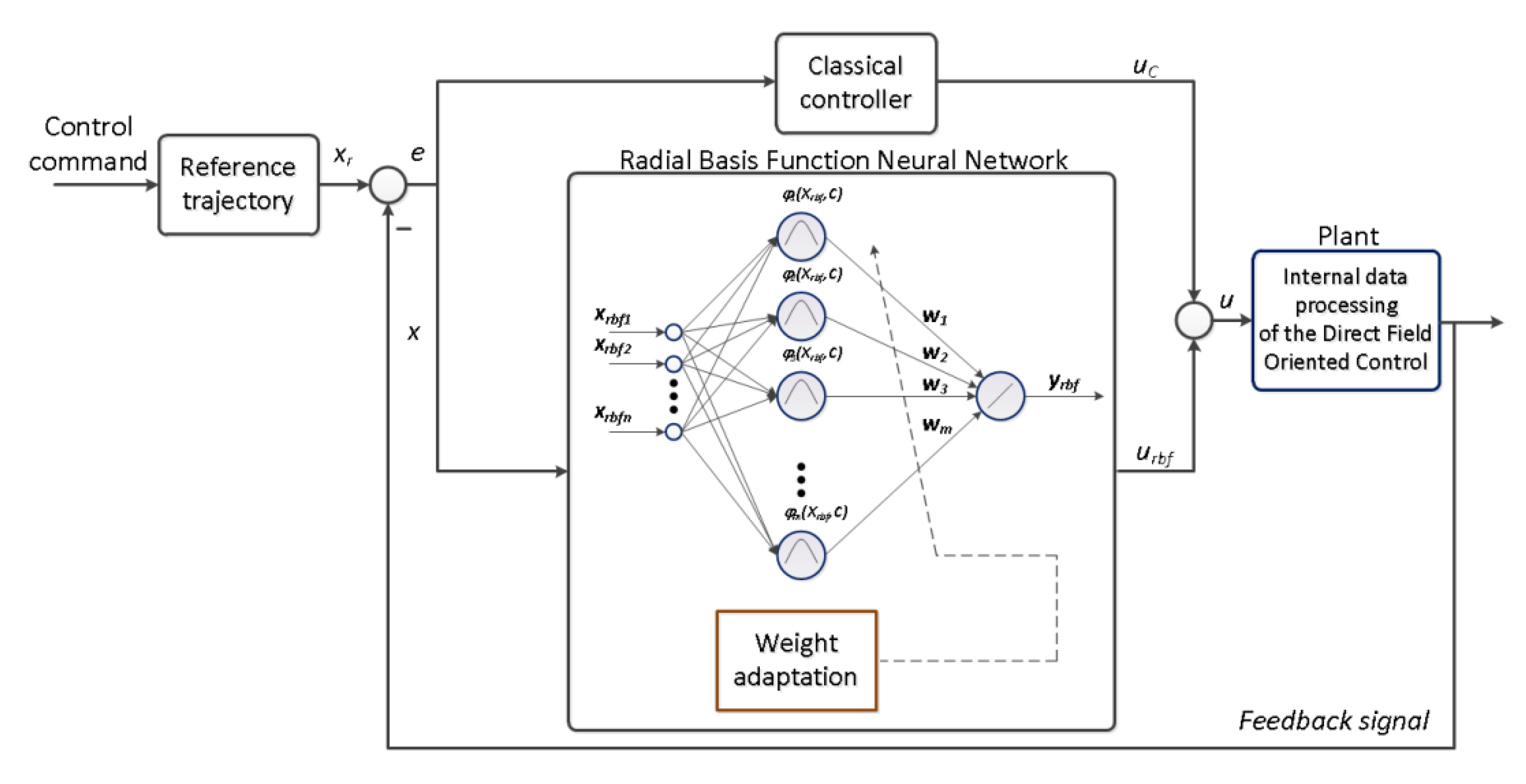
The analyzed speed controller was based on the neural network, with a radial basis activation function applied in the hidden layer. The input vector contained two signals: the speed error and the same signal from the previous step of calculations (a unit delay was applied). The goal during the on-line training (according to the rules described in this section) was minimizing the cost function that described the difference between the input signal and the actual speed trajectory. The Radial Basis Function Neural Network (RBFNN) controller was connected to the rest of the system in series. This meant that the object was a disturbance for the network. However, the adaptation law aims to obtain the set value at the output of the system. Therefore, the output of the net was a part of the control signal; it was a component of the reference value for the internal part of the FOC algorithm. The overall algorithms consisted of a PI controller and a neural network combined in parallel. The centers in the RBFNN were constant. However, assuming a fast update of the weights, the controller was able to adjust the operation to the nominal parameters of the object. Occurring disturbances were also quickly eliminated. In this case, the neural network was an adaptive compensation element. A mathematical description of the calculations performed in the speed controller is presented below. Moreover, the stability analysis was an important element of the design process described in this article.
The simplified topology of the controller is presented in Figure 2. The general form of the object can be assumed as:
x ˙ ( t ) = f ( x ) + g ( x ) u p
where: f(x) and g(x)—the plant and control functions, respectively, x—the state vector and up—the input of the plant.
The error changes during the control system calculations can be described with the below expressions:
e = x r x
e ˙ = x ˙ r x ˙
where: xr is a reference state of the plant.
Using (7) and the additional assumptions ( t , e ( t ) 0 , e ˙ ( t ) 0 ), the calculations presented below can be performed [14]:
x ˙ = x ˙ r + u r
where: ur(t)—the reference (desired) control signal.
By combining (8) and (5), the following formula is achieved (the symbol ^ means estimation):
x ˙ ( t ) = f ( x ) + x ˙ r ( t ) + u r ( t ) f ^ ( x )
Based on the above, the error dynamics are defined by the below expression:
e ˙ = f ( x ) u r ( t ) + f ^ ( x )
The signals from the classical PI controller uc and the neural model urbf are combined in the analyzed control structure (applied in the speed loop of the induction motor):
u r u = u c + u r b f
where:
u c = k p e ( t ) + k i e ( t ) d t
and kp—the gain of the proportional part and ki—the gain of the second path of the controller (kp > 0, ki > 0).
In this work, for neural calculations, the RBFNN model was applied. Several nodes of a hidden layer contain assigned centers (for the k-th element) [46]:
C k = [ c k 1 , c k 2 , c k 3 c k n ]
Additionally, the width of the Gaussian function can be scaled using the parameters b (bk > 0):
b = [ b 1 , b 2 , b 3 b m ] T
Thus, for the input vector (n-size):
X r b f = [ x r b f 1 , x r b f 2 , x r b f 3 x r b f n ] T
the outputs of the following radial neurons are described by the expression:
φ k = exp ( X r b f C k 2 2 b k 2 ) , k = 1 , 2 , 3 , m
where: . means the distance between the input values and the centers of the neurons.
In the last part of neural processing, the values φk are multiplied by the matrix of weights:
W = [ w 1 , w 2 , w 3 w m ] T
and the output is calculated as:
y r b f = k = 1 m w k exp ( X r b f C k 2 2 b k 2 )
The considered application assumes on-line data handling (including the weight adaptation, described below), so for the i-th step of calculations, the RBFNN output is achieved using the equation:
y n n ( i ) = y r b f ( i ) = W ( i ) T φ ( i ) = w 1 ( i ) φ 1 ( i ) + w 2 ( i ) φ 2 ( i ) + w 3 ( i ) φ 3 ( i ) + + w m ( i ) φ m ( i )
and the adaptation of the neural network weights, in several iterations i, can be described as:
w ^ k ( i + 1 ) = w k ( i ) + Δ w k ( i )
Concluding, the real output of the RBFNN can be formulated using the expression:
u r b f = W ^ T φ
where: W ^ and φ—matrices of the calculated weights and hidden layer outputs, respectively.
Then, Equation (10) is modified as below:
e ˙ = f ( x ) u c u r b f + f ^ ( x )
Defining the error (using matrix):
E = [ e e ]
Then, (22) is represented as:
E ˙ = Λ E + B ( f ^ ( x ) f ( x ) u r b f )
where:
Λ = [ 0 1 k i k p ]
and
B = [ 0 1 ]
The purpose of the RBFNN application is the reduction of the error applied in the control signal calculation. It works like a compensator:
Δ = f ^ ( x ) f ( x ) = u r b f o + ε
where: urbfo—the optimal signal of the RBFNN (with the precise weight matrix Wo):
u r b f o = W o T φ
Precise control means a significant reduction of the training error ε; thus, the bounds of the mentioned error should be assumed [47]:
ε b Δ _ _ sup X r b f f ^ ( x ) f ( x )
Then, using (27) in (24), the following formula is obtained:
E ˙ = Λ E + B ( u r b f o u r b f + ε )
The following definitions of errors should also be introduced:
W ˜ = W o W ^
W ˜ ˙ = W ˙ o W ^ ˙
After the next update, Equation (30) has form:
E ˙ = Λ E + B ( W ˜ T φ + ε )
A stable adaptation law can be derived after the Lyapunov function assumption:
L = 1 2 E T P E + 1 2 t r ( W ˜ T Ξ W ˜ )
where: P—a positive definite matrix, Ξ is a non-negative matrix and tr means the trace of the matrix.
The derivative of the Lyapunov function is calculated below:
L ˙ = 1 2 E ˙ T P E + 1 2 E T P ˙ E + 1 2 E T P E ˙ + t r ( W ˜ T Ξ W ˜ ˙ )
By using the derivative of the error (33), the above formula can be recalculated (for the next part of the calculations, the sizes of the matrices are neglected—to simplify the mathematical description):
L ˙ = 1 2 Λ E P E + 1 2 B W ˜ φ P E + 1 2 B ε P E + + 1 2 E T P Λ E + 1 2 E T P B T W ˜ φ + 1 2 E T P B ε + + t r ( W ˜ T Ξ W ˜ ˙ ) = Λ E T P E + B T W ˜ φ T P E + B ε P E + t r ( W ˜ T Ξ W ˜ ˙ )
The P matrix is calculated using the equation:
Q = ( Λ T P + P Λ )
where: Q—a positive definite matrix.
Then, the formula (36) can be rewritten:
L ˙ = 1 2 E T Q E + B ε P E + B W ˜ T φ P E + t r ( W ˜ T Ξ W ˜ ˙ )
The following mathematical rule (for column matrices a and b) is known:
t r ( b a T ) = a T b
and similarly, for square (m × n) matrices A and B:
t r ( A T B ) = i = 1 m j = 1 n A i j B i j
Based on the above, Equation (38) can be formulated as follows:
L ˙ = 1 2 E T Q E + B ε P E + t r ( W ˜ T Ξ W ˜ ˙ + B W ˜ T φ P E )
Let the proposed stable adaptive law be as follows:
W ^ ˙ = 1 Ξ B φ P E
After the recalculation of (41), using (42) and (32):
L ˙ = 1 2 E T Q E l 1 + B ε P E l 2
For the stable work of the control structure, negative values of L ˙ are necessary:
L ˙ 0
Thus, it is obvious that l1 from (43) is not positive (l1 ≤ 0). For a small value of the training error (in the above calculations, the limits are introduced (29)), the control system is stable.

4. The Grey Wolf Optimizer

4.1. Details of Data Processing in the GWO

Modern optimization techniques, based on nature observations, assume the modification of the data set in each iteration of the calculations. According to specific rules, the space of potential solutions is processed. After each turn, the results are evaluated. A characteristic feature can be observed: the elementary operations are often very basic and dependent on the best values from the previous step. Observations of the natural behavior of a group of individuals (wolves) are the base for the optimization algorithm tested in this application.
The detailed rules are presented in Algorithm 1. After removing the data from previous tests, the simulation’s condition is declared (the frequency of the calculations, solver, operation time of the model, etc.). Before starting the data processing in the GWO, a dedicated file with the plant should be prepared. It should contain proper reference signals and defined parameters (e.g., the mechanical time constant of the electrical machine). Then, important for the final results, the GWO parameters are introduced. They include the maximum number of iterations, size of population, number of optimized parameters and bounds for solution. After the above actions, the GWO population is initialized as a set of random numbers. Each value is evaluated by the previously declared objective function. Thus, the first best solutions are found. Then, the main loop starts. In each iteration, the elements of the data are recalculated. In the following step, all the solutions are tested again as parameters of the speed controller. The obtained controller gains are closer to the optimal. This information is used in the next step of the algorithm. Before starting the next iteration, the aGWO coefficient is updated, and the conditions ending the computation are checked. After the saving of all the operation’s results, the final report is generated. Equations presenting the details of the calculations performed in the GWO are presented in the next paragraph.
Algorithm 1. Grey Wolf Optimizer
1:  INITIALIZATION STAGE:
2:   environment preparation:
3:     preparation of workspace
4:     conditions of simulations for model (frequency, solver, etc.)
5:     reference signals definition
6:     parameters of the plant
7:   initial state of the GWO:
8:     overall conditions of calculation (number of iterations (imax), size
9:     of population, number of optimized variable, bounds for solutions)
10:    random initialization of controller gains
11:    initial calculations of aGWO, AGWO, CGWO
12:    the GWO-calculations for best solutions finding
13: MAIN CALCULATIONS of the GREY WOLF OPTIMIZER:
14:  for i = 1 to imax do
15:    update of features for each element of population
16:    calculations of cost function for each element of population
17:    finding new best solutions
18:    update of aGWO
19:  end for
20: SAVING RESULTS:
21:   presentation of results
22:    data for summary file
23:    report generation
Before the main loop of the GWO, the cost function fc is calculated, and the best individuals are determined (based on the reference speed ωref and the actual value ω):
f c = 0.5 k = 1 n G W O ( e k G W O ) 2
where: nGWO—the total number of samples and k—the number of analyzed samples; moreover:
e k G W O = ω r e f k ω k
The parameters for cyclical changes of the coefficients of the processed data set are described using the following equations [48]:
r 1 = r a n d
r 2 = r a n d
A G W O = 2 a G W O r 1 a G W O
C G W O = 2 r 2
where: r1 and r2 are uniformly distributed random numbers.
In Equation (49), the agwo is used. It is a coefficient narrowing the area of search for the best solutions (the values decrease from 2 to 0):
a G W O = 2 2 i i max f o r i = 0 i max
In the next step, using values (47)–(50), the following expression is calculated:
D α = | C G W O X α X G W O |
where: —the best solution from the previous loop (in the first step, randomly selected solutions are used) and XGWO—the whole set of solutions.
The achieved parameter is applied in:
X 1 = X α A G W O D α
Again, (47)–(50) are recalculated for the equation:
D β = | C G W O X β X G W O |
in which Xβ is the second optimal solution. Similarly, like above, X2 is calculated:
X 2 = X β A G W O D β
Finally, the procedure is repeated for X3. Once more, the equations for the parameters r1, r2, AGWO and CGWO are used for (assuming with the third optimal values):
D σ = | C G W O X σ X G W O |
and
X 3 = X σ A G W O D σ
The update of the population is calculated according to the formula (for the i-th iteration):
X G W O i + 1 = X 1 + X 2 + X 3 3
In this application, the grey wolf optimizer is applied for the optimization of part of the parallel neural controller. More precisely, the fixed parameters of a classical PI controller are determined.

4.2. Analysis of Optimization Process

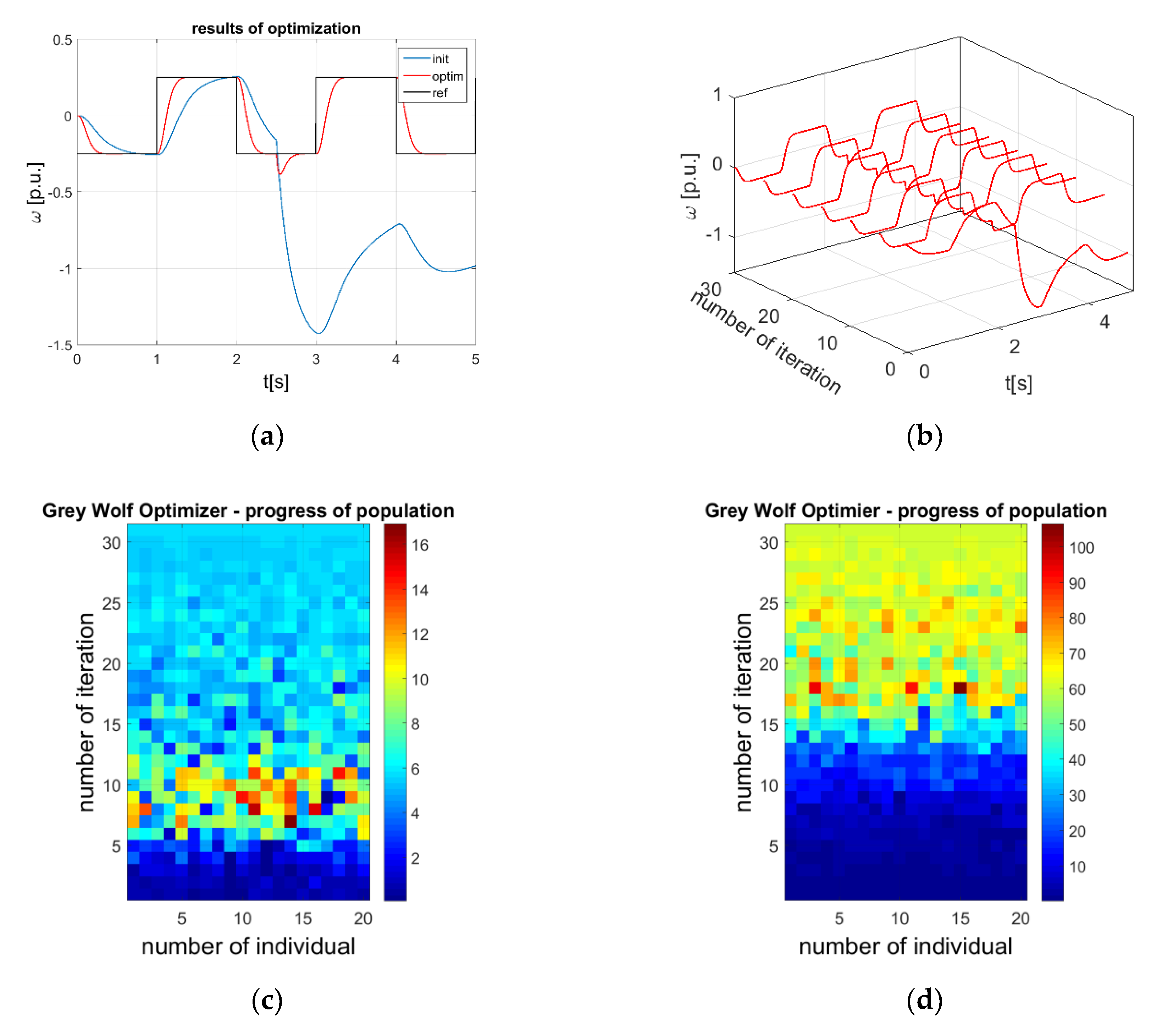
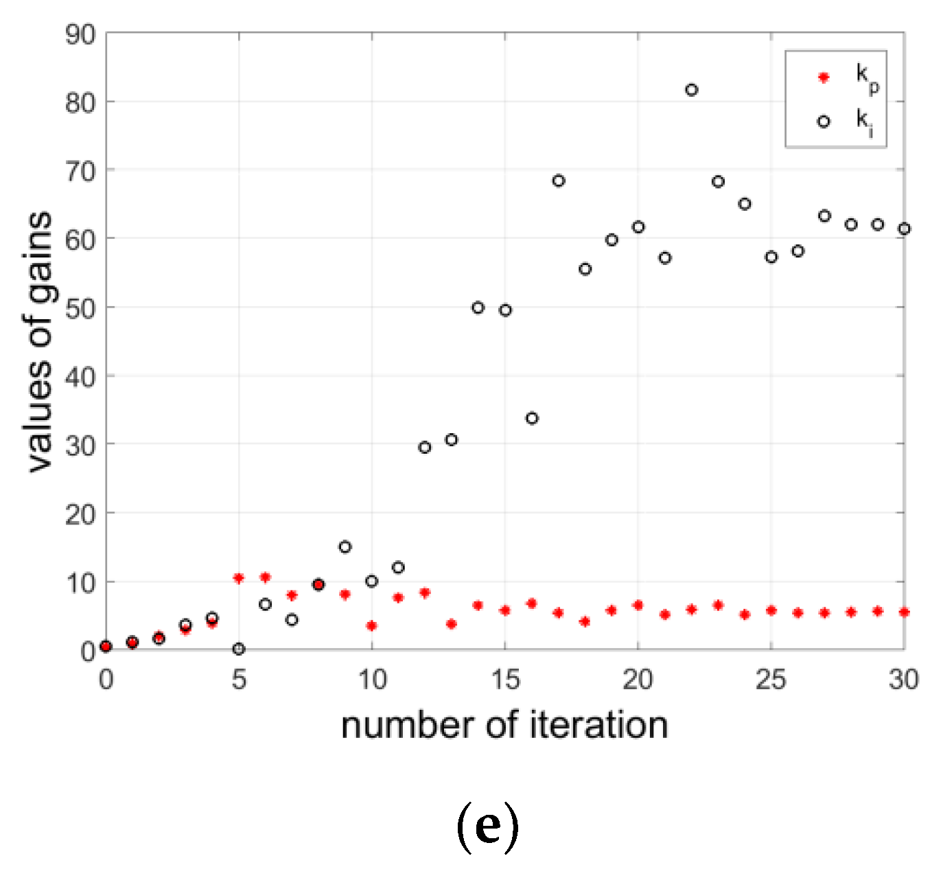
The calculations of the GWO algorithm are preformed iteratively. After each sequence of processing, the population is modified. In this section, the influence of those operations on the controller parameters and the achieved results is analyzed in several stages. From the results (Figure 3), it is possible to read significant calculation conditions, in particular, the maximum number of iterations (the first line also contains the starting point—before optimization) and the size of the group. However, additional information deals with the bounds of solutions. The lower limit was set to 0.05, and the upper possible value was 500. The tests present the control system’s response to cyclic reversions. The reference speed at steady state is 25% of the nominal value. Half of each test is measured under the active work of the load machine. As mentioned before, the initial values of the speed controller parameters were chosen randomly (kp_init = 0.4663 and ki_init = 0.6136). The reference trajectory was not tracked precisely (Figure 3a). At each step, the GWO calculations obtained the improved solutions (Figure 3b). The settling time was reduced, and a significant change was observed after t = 2.5 s (load switching). Overshoots were not observed. Finally, after 30 iterations, the following values were obtained: kp = 5.5892 and ki = 61.4973. The transient of the motor speed is satisfactory for those levels of controller parameters. Initially, the fluctuations of both gains were significant (Figure 3e). However, when analyzing the trend of changes in the final stage of processing, stabilization can be easily observed. It means that the group is approaching the optimal solution.
The transients shown in Figure 3c,d allow the observation of changes in the entire population during the subsequent calculation steps. The X-axis of the chart represents the individual number, while the Y-axis (upwards in the subsequent layers of the colormap) is related to the results in the following stages of the mathematical operations (equations presented in the previous section). Figure 3c shows the results for the gain in the proportional path of the controller, while the next one (Figure 3d) presents a graph for the parameter of the integral element. Random numbers were assigned to the whole initial population of wolves. It should be clarified that the above-mentioned initial values of the potential controller parameters resulted from tests for subsequent values in the group. The settings corresponding to the smallest value of the objective function were adopted as the initial solutions (kp_init and ki_init). The parameters in the entire space of the analyzed solutions are stabilized. It is important that in the intermediate stages of calculations, samples of larger (than the optimal values obtained in the last iteration) values are visible. It means that the population returns to the area of the best solutions, and then narrows down the searching for the optimum in this region.

4.3. Common Problems of Metaheuristic Methods Applied for Classical Controller Tuning

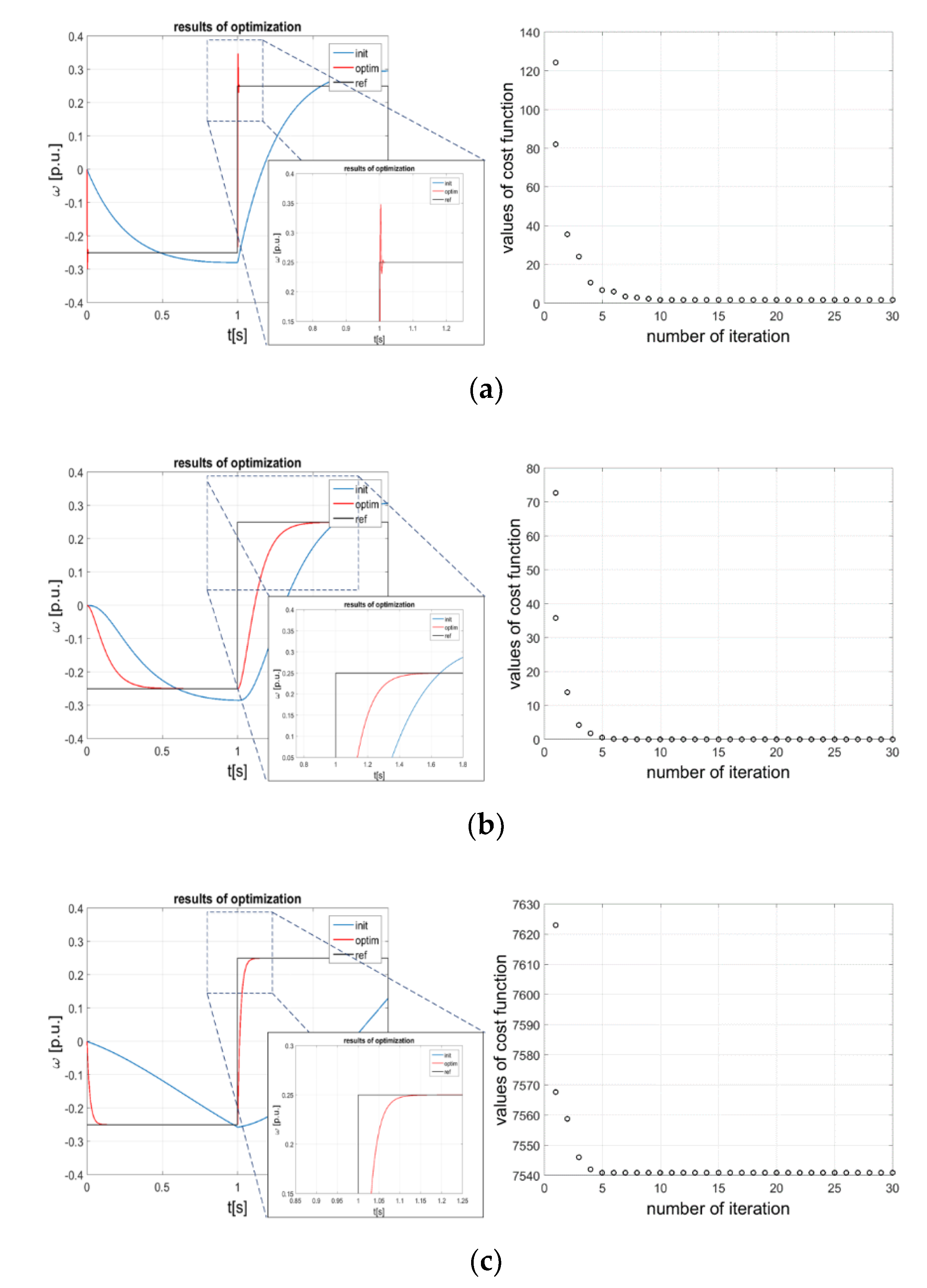
Most often, during tests of control structures for an electric drive (but also for other dynamic objects), the shape of the forcing signal is step or square. It allows testing the properties of the control system under dynamic changes of state variables. In the case of the mentioned reference speed signals, a characteristic phenomenon is observed during the optimization of the control structure parameters. It is obvious that the ideal tacking of the input transient cannot be achieved. It is related to the time constants of the electromagnetic torque-shaping loop and—the greatest one—the mechanical time constant. Calculating the speed error for each sample—in fact, the area between the reference value and the actual level of the signal—is considered. Closer analysis leads to the conclusion that the short-time peak (Figure 4a) can be thought of as a lower value of the calculated control error than, for practical reasons, the results of a properly optimized one (Figure 3). However, it can be dangerous for closed-loop control. A high value of the short-time signal can lead to oscillations or instability. The second problem, in such a situation, can be related to damage to the shaft and the mechanical elements of the drive (jerks caused by the peak). It should also be noted that the above issue is triggered by large values of optimized parameters. High values of gains can amplify measurement noises. The use of algorithms based on biological observations often leads to the described problem. The following methods are used for the proper optimization process realized for sharp forcing signal shapes:
The modification of command signals (the application of input filters or slope trajectories);
The insertion of additional noise to the feedback paths;
The alternative definition of the cost function.
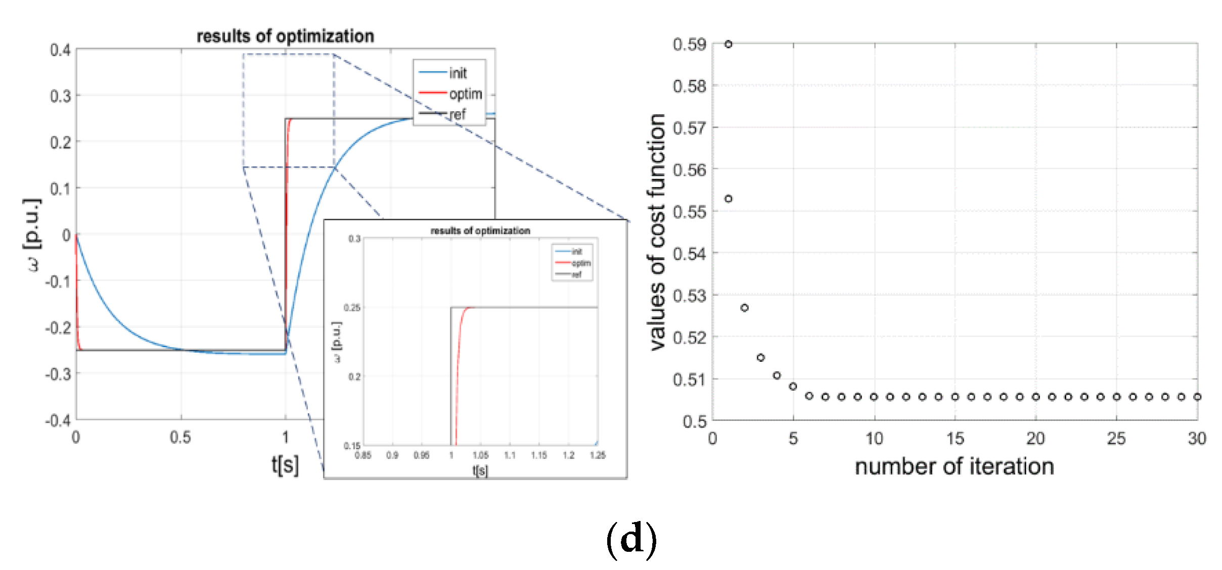
Figure 4 shows an example of the implementation and optimization of a PI controller used for a dynamic plant. The first method (Figure 4b) assumes forcing the speed according to a soft input signal [49]. It is simple to implement. In addition, the parameters of the input filter model or ramp slope affect the achieved gains. Here, the input signal-shaping element was defined using the following transmittance:
G i n ( s ) = ω 0 2 s 2 + 2 ξ ω 0 s + ω 0 2
where ξr is the damping: coefficient and ω0 is the reference resonant frequency.
In the second case, an additional disturbance was introduced in the feedback loop (Figure 4c). Noise was added to the speed measurement path. Such action is inspired by the phenomenon described in [50]. Increasing the gain value in control systems can lead to better dynamic properties. However, in a real (hardware) application, there may be a problem with measuring the noise amplification (it affects the control error). In relation to the tuning of the controller using metaheuristic methods, the described phenomenon can be used to limit the excessive growth of the optimized values.
The last example takes into account definitions of the cost function (Figure 4d) other than (45). The modified formula is shown below:
f c 2 = 0 t ( e f c 2 ( t ) t 2 + χ | Δ e ω | t 2 + ς | Δ u s | t 2 ) d t
where:
e f c = ω r e f ω
Δ e ω = d d t ( ω r e f ω )
Δ u s = d d t u s
us—the control signal, and χ and ζ are constant parameters.
In Equation (60), the last two components are characteristic elements. The first of them allows taking into account, during optimization, the influence of the error derivative value. Thus, rapid changes are reduced. Additionally, dynamic changes in the control signal are reduced [39]. According to this method, the effect of short-term overshoots (Figure 4a) is eliminated.
It should be noted that this is not a comparison, but a presentation of effective methods for avoiding the described problem (Figure 4). All methods present a preset speed level obtained without overshoots. In the following tests, various starting points were assumed; this is visible in the values of the objective function. The speed control error, for the best solutions, is reduced, so the controller is properly tuned. It is worth paying attention to the overall level of the final values of the cost function in subsequent simulations. The values do not oscillate around zero in each case. The introduction of noise increases the numerical value of the error (even around the best results).
The results in the previous section were obtained for the model of the drive with IM. A combination of the above-described methods was adopted. Noise (uniform random numbers) and the input model (ω0 = 15 s−1, ξr = 1) were used. The fc objective function was used in the optimization.

4.4. Starting Point of the Grey Wolf Optimizer

The initial assumptions have to be defined for the optimization problem. The starting point can have an influence on the final results. When applying metaheuristic algorithms, the initial values are most often selected as random numbers. It is a situation similar to that during the optimization of neural network weights (training). Initial randomization was also consistent with the assumptions of this project. Three rules were defined during the GWO optimization; the details are presented below.
The values of the speed controller gains were selected from the uniformly distributed pseudorandom numbers. This ensured a lack of the initial information about the problem.
The parameters have to be positive. This is due to the structure of the controller (PI).
The random number should be a fractional value (the calculation starting point is distant from the optimal solution). It seems to be the most difficult case to optimize.
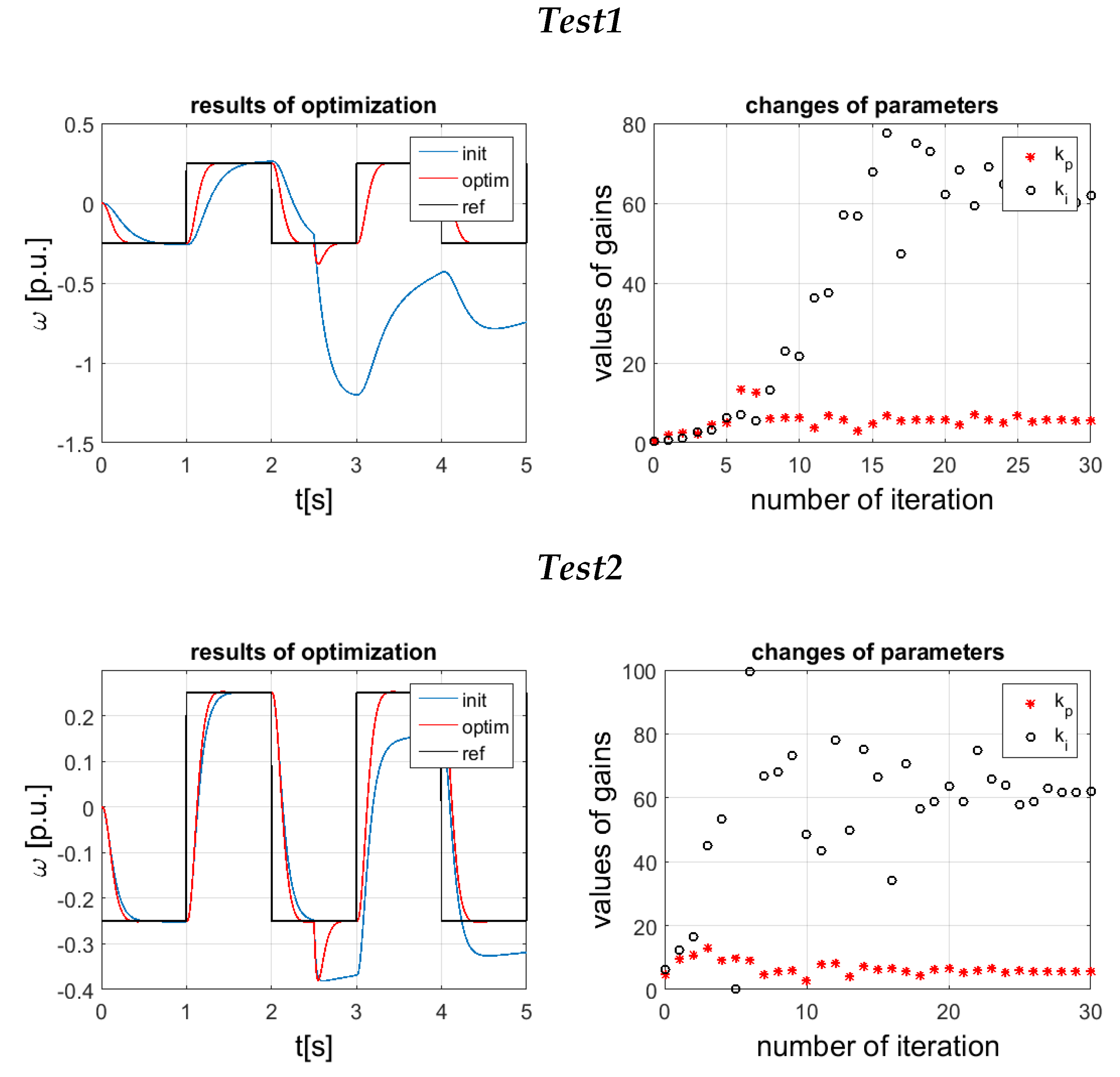
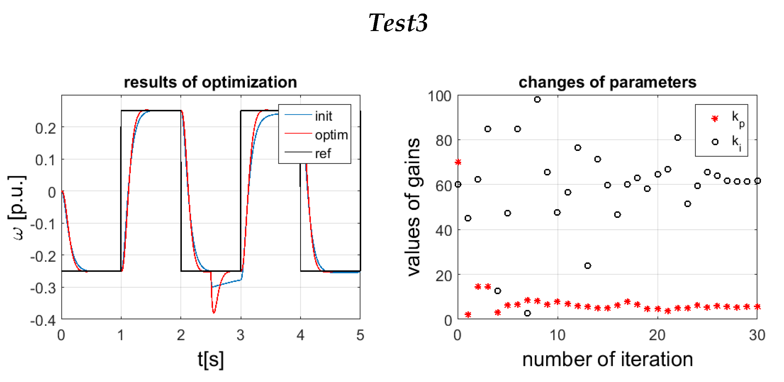
In order to analyze the influence of the initial values of the GWO algorithm, additional tests were performed. The results are shown in Figure 5; the details are presented in Table 1. In subsequent tests, the principles described earlier were applied. However, the numbers obtained in the randomization process were re-scaled. In this way, significantly different initial conditions for the optimization algorithm were obtained. The following calculations of the GWO algorithm led to very similar gains for the optimized controller. This is an important feature of the implemented technique—the repeatability of the results.

5. Simulations

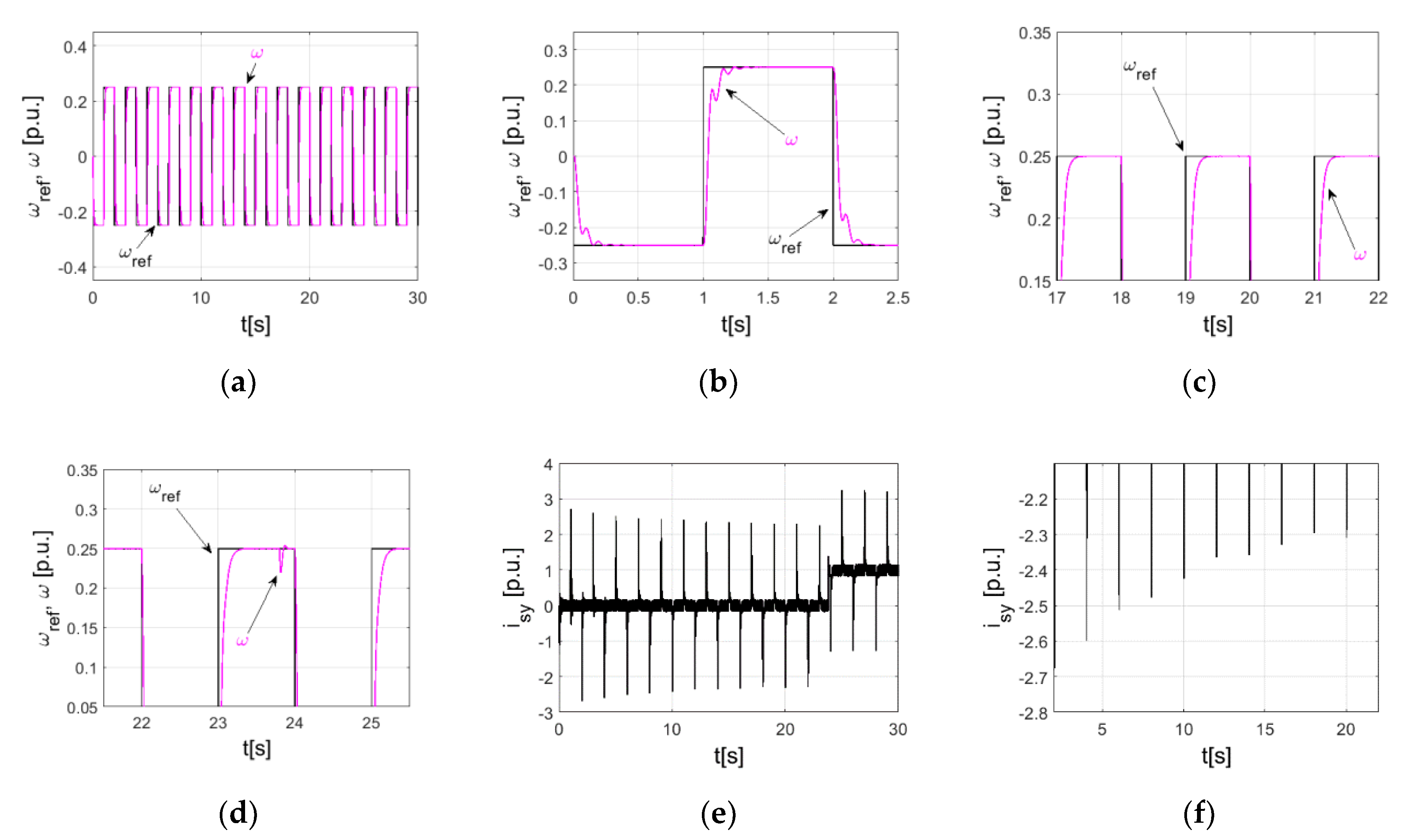
The verification of the control method, described in this paper, was performed firstly in simulations. Both parts of the parallel speed controller described in the previous sections were combined. The described neural controller was used in the speed control loop of the DFOC method. The drive model, according to the scheme presented in Figure 1, was prepared. Five nodes in the radial layer of the neural network were applied. The parameters of the PI controller were set as described in the previous part of the article. The most important data of the control system are presented in Table 2. The fixed step size of the calculations was set to tc = 0.0001 s. The tests took 30 s. The reference trajectory forces the drive to cyclic reversion. The speed in steady state was 25% of the nominal value. The values of the state variables were analyzed in a per unit system (all the saved data are divided by the nominal level). The starting part was realized without the active work of the load machine. Then, during the work of the drive, the load torque was added at time t = 23.8 s. The design parameters in Equation (42), the constant part defined by user, are represented here using one symbol, η. Two state variables were analyzed in the tests: the speed of the motor ω and the isy component of the stator current. These signals are a reference to the cascade structure of the DC motor control (electromagnetic torque and the main controlled variable—speed).
The first test was prepared for the nominal parameters of the drive. The purpose was the presentation of the correct work of the control structure. The training parameter of the neural network was equal to η = 0.09. The long-time period of drive operation is presented in Figure 6a. It is a practical validation of the stable work of the drive. The three next transients contain, for the easier analysis of the results, an enlarged fragment of the speed signal. The mentioned figures show the following stages of the test: the initial phase (Figure 6b), the tuned neural network (Figure 6c) and the switching of the load (Figure 6d). Precise control is observed. The reaction of the drive after the load acting is very short. Figure 6e shows the transient of current. The adaptation can be easily noticed. Improved after each reversion, reference speed tracking is possible because of the modification of the current shape in the control system (Figure 6f).
For the part of the control structure related to speed, the most significant part is the mechanical part of the machine. In the previous trial, this parameter was at the level tm = tmn = 0.15 s. Now, the work of the control system was analyzed under variation from the nominal (Figure 7). The other conditions were the same as in the above test. If the value of this parameter is twice as large, the motor is heavier, the downcast in the speed signal is smaller (after load switching) and the temporary values of the current are higher (Figure 7a–c) than in the second (tm = 0.5tmn) case (Figure 7d–f). Overall, the conclusion is as follows: the adaptation (modification of the weights) of the controller coefficients leads to the proper operation of the motor, even if the fluctuation of parameters occurs in the drive. The neural network can compensate for the changes in the mechanical time constant.
Subsequent studies dealt with issues typical for neural controllers. In the first part of this section, the results (in the initial part of the drive acting) contain oscillations. This is a typical problem noted in applications of neural controllers. The reason is related to the initial values of the neural network coefficients. The weights are randomized. The results, presented in Figure 8a–c, were obtained for different initial conditions (subsequent draws). During the first period of the speed transient, the impact of such action is slightly visible. However, the system is stable and convergence (of the reference and actual speed) is quickly achieved. This does not affect the further operation of the system (after a few seconds, the response against the load is identical). The solution to such a problem is the initial pre-training of the neural network; then, the adaptive law starts with predefined values for the weights.
The dynamics of the adaptation algorithm have an impact on the parameters of the neural network. They are dependent on the training rate. The influence of the constant η is visible in Figure 8d–f. Small values of the learning parameter cause longer adaptation times, while increasing the value forces faster adaptation. However, a very high value of the training factor can cause overshoots and oscillations of the state variables. An increase in the constant coefficient used in adaptation increases the step of the optimal value search (it reduces the time for proper value calculation). However, the optimization algorithm may, in this case, omit the global optimum. Otherwise, a small value of η leads to not-very-large increments of weights in the neural network, and as a result, the precision of the calculations is higher.

6. Experiment

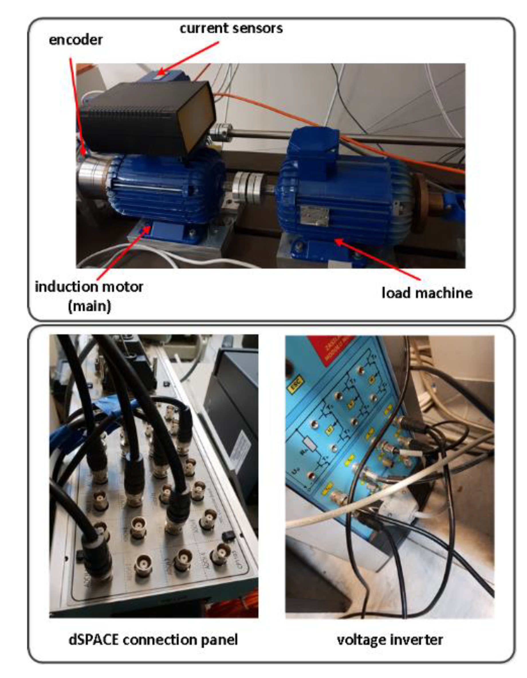
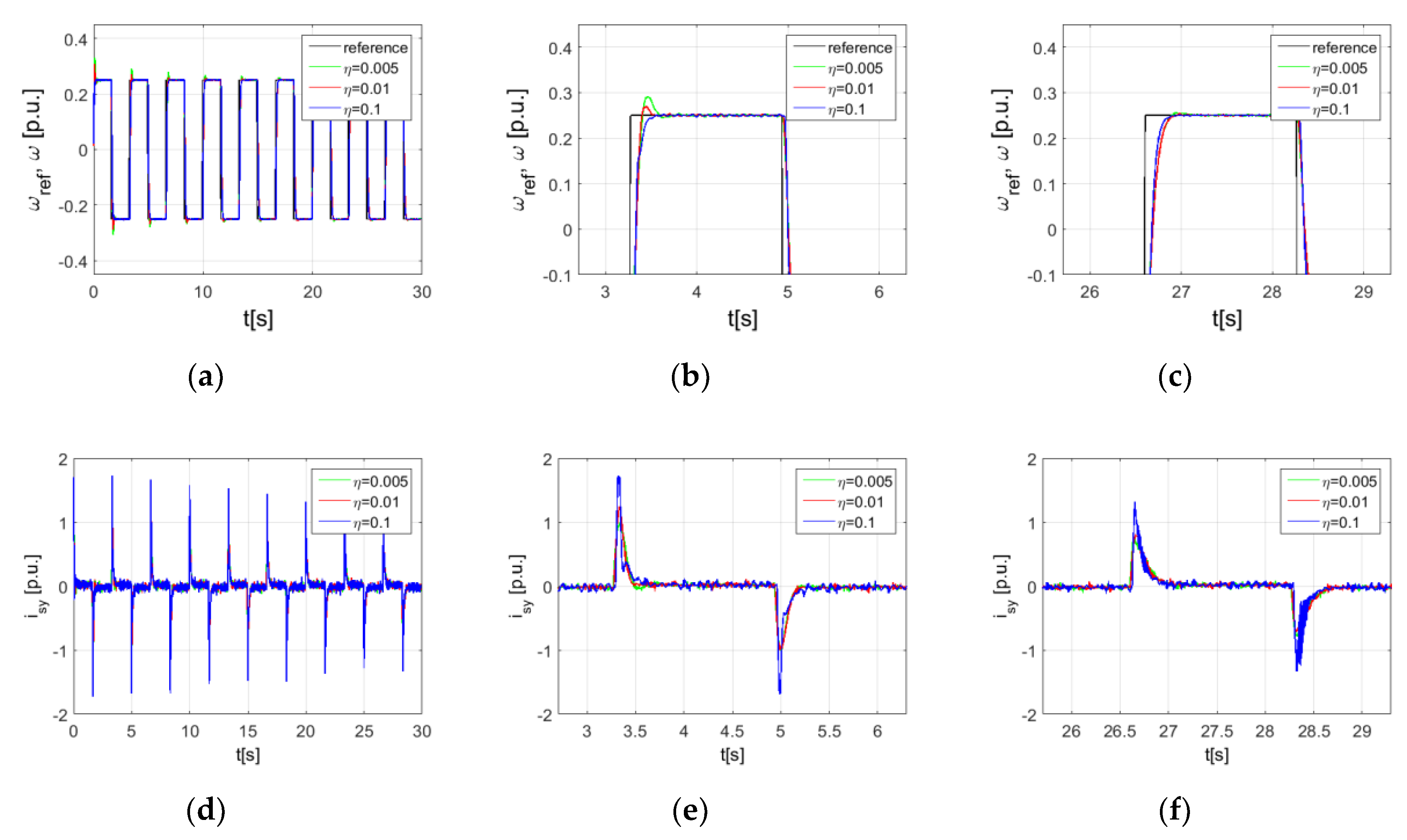
As a real implementation of a neural control system (the details are presented in previous sections), the experimental tests prepared for an induction motor are investigated in this section. The control algorithm, presented in Figure 1 (optimized using the grey wolf optimizer), was implemented in the digital signal processor of the dSPACE1103 card. The sampling time assumed in the data processing of the structure was set to tc = 0.0001 s. The signals were measured using an incremental encoder (36,000 pulses per rotation) and a current sensor. These elements were connected to the processor using an external board. In the subsequent stage, after the calculation of the neural controller and the following part of the DFOC, a control signal for the voltage inverter was generated. The main part of the laboratory set-up consisted of two electrical machines (a motor and load) connected using a rigid shaft (Figure 9). The experimental tests were realized for the induction motor with a nominal power of 1.1 kW.
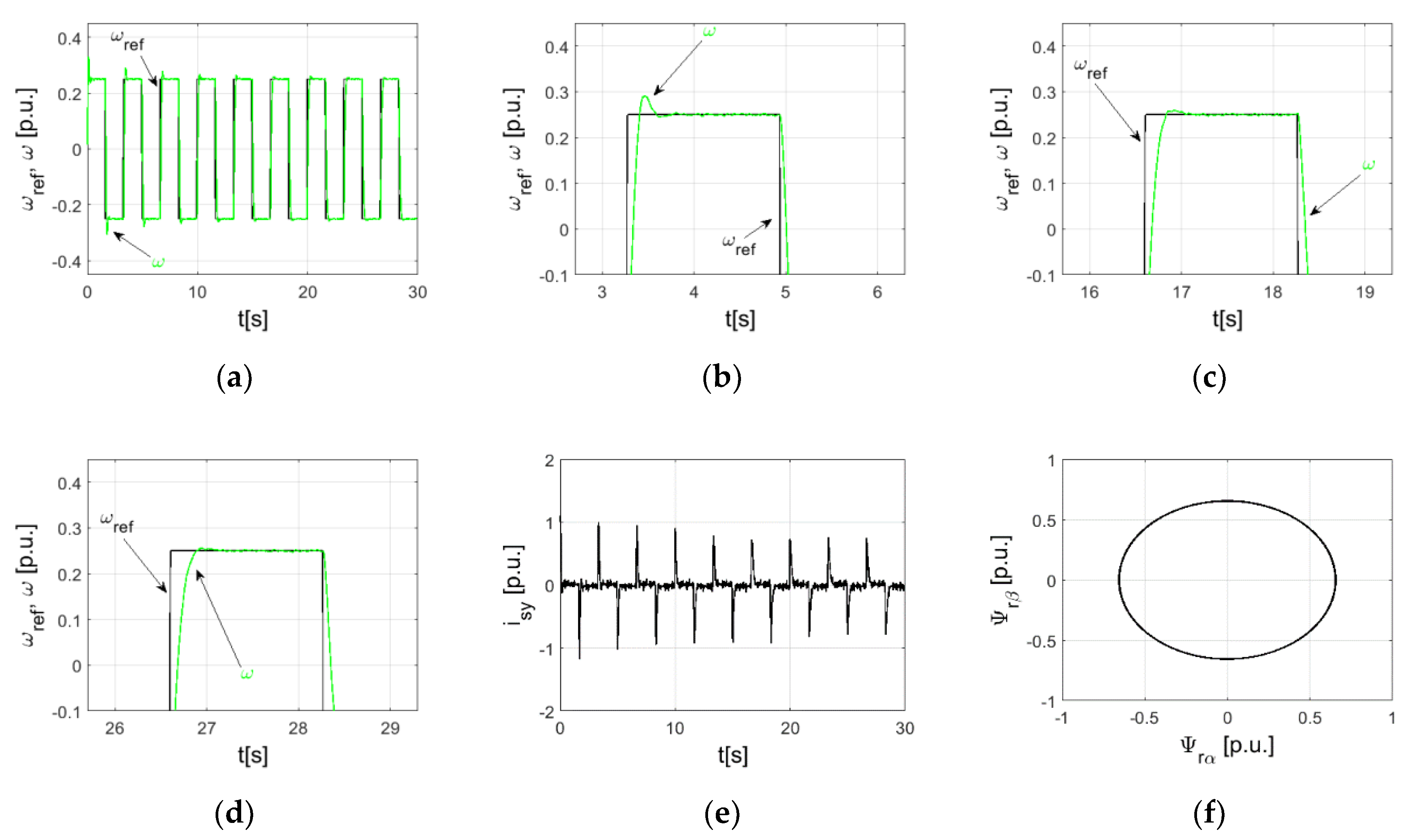
In the first scenario of the experimental tests, a square waveform was set as the command signal. The load was not turned on. As shown in Figure 10a, the adaptation of the internal coefficients of the neural network compensator leads to precise control. The control method could obtain the command speed (with acceptable error) in a relatively short period of time. Then, the work of the control structure under external disturbances was also analyzed (Figure 11). In each upper half of the reference course, in the steady state, the load was switched on, and after a short time (about 0.5 s), it was disconnected. Comparing Figure 10b,d (and Figure 11b,d, respectively), a reduction in overshoots is easily noticeable. For both analyzed cases, the isy current is also presented. In this configuration of the drive (DFOC), the dynamics of the changes and the shape of this signal are similar to the electromagnetic torque. Thus, during machine speed changes (e.g., the start of the motor), its value is increasing. Then, if the load is not active, only natural phenomena are obstacles (e.g., friction). As a result, the value of this component of the stator current is minimal (Figure 10e). However, more power is needed if the load is turned on; the step (increasing) of the current is visible (Figure 11e). The relationship between the components of the rotor flux also indicates the correct operation of the control system (Figure 10f and Figure 11f).
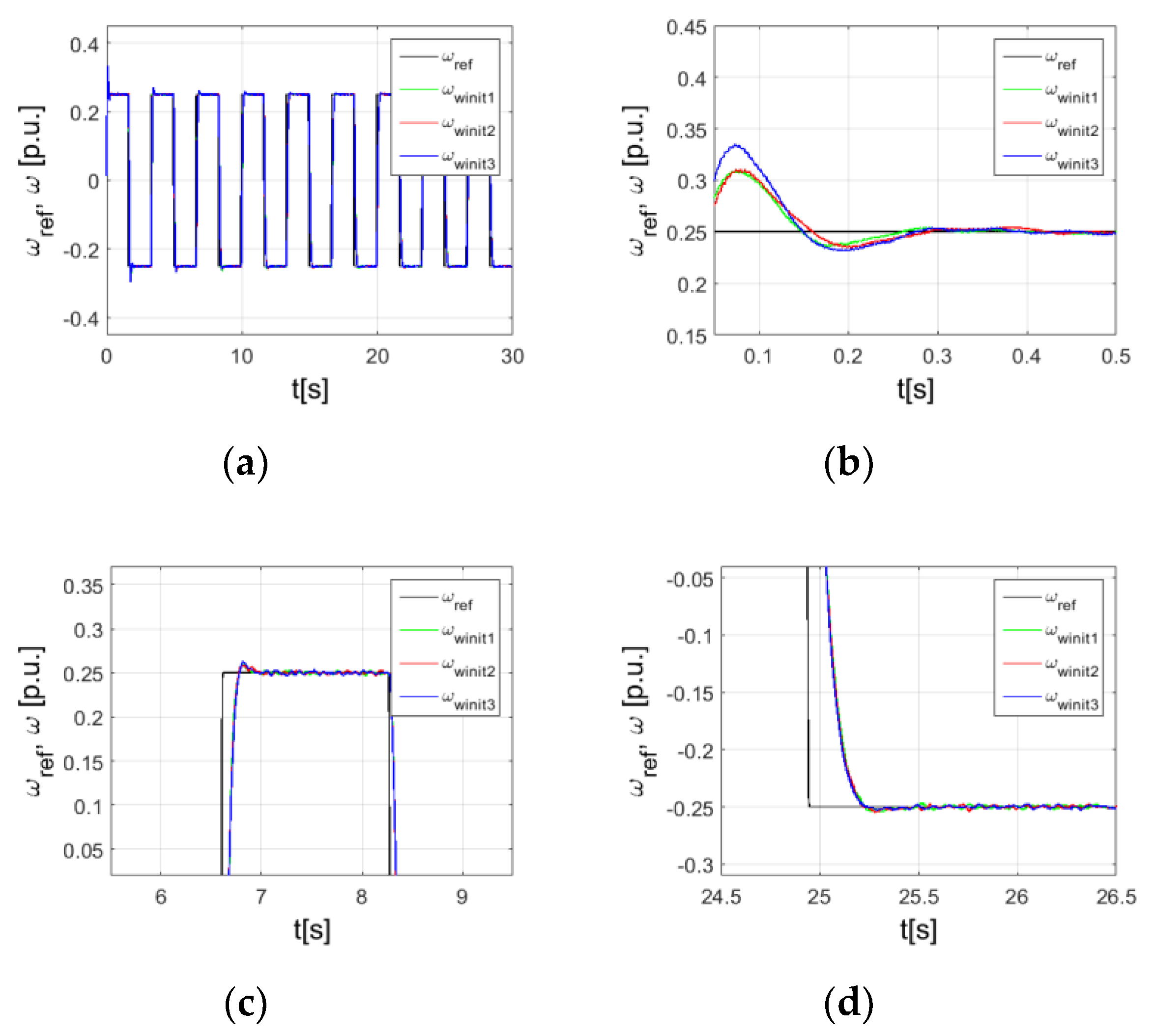
To evaluate the start of the drive with a different initial point of the neural part used in the speed controller, the tests of the plant were repeated. All the conditions of the tests were fixed, but the weights were randomized (for each benchmark). Figure 12 presents the repetitive actions of the drive. In the initial part (Figure 12b) of the transients, the shapes of the signals are divergent. The following sequences of the motor operations show improvement; for all the tests, the results are similar. The optimization algorithm, applied for the weight update, is at the same point for each case. However, the overshoots are still visible (Figure 12c). In the next few seconds, the problem is eliminated. The results are almost identical, and the accuracy of the speed control is very high (Figure 12d).
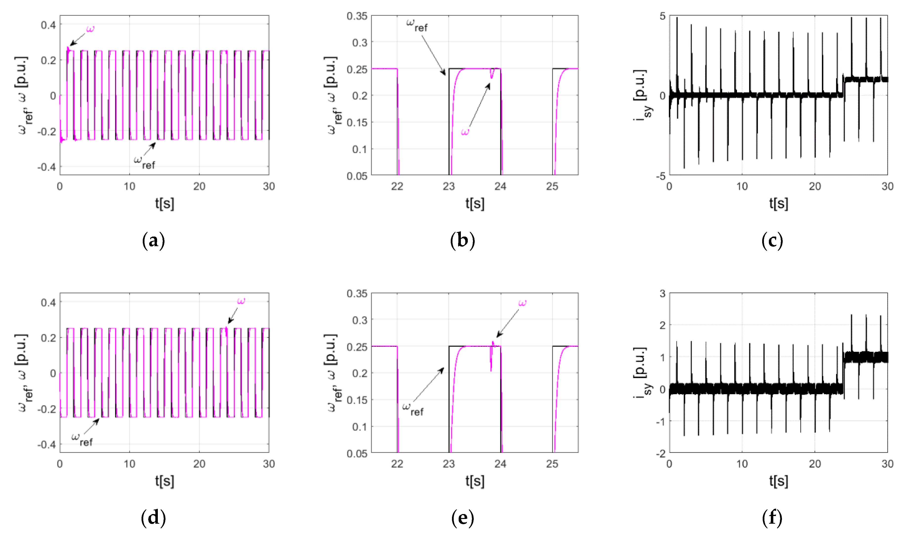
The previous results in this section of the article were obtained for the same conditions as those assumed in the simulations. Now, the influence of the η parameter on the dynamics of the drive was tested in the experiment. The results are presented in Figure 13. A periodic step command was sent to the drive. A quick response of the induction motor was observed. Additionally, the impact of the controller parameter adaptation was significant. The output of the speed controller was a reference signal to the torque control part. If this state variable was processed very fast (compared to the speed control loop) and without disturbances, the effect (changes in the current values in temporary states) is visible in the changes in current isy (Figure 13d). Then, this signal influenced the speed transients (Figure 13a). It is worth mentioning that the general observations are close to the simulations. A higher value of the constant parameter in the equation used for the weight recalculation can reduce the time of adaptation. However, this parameter should not be overstated. This can lead to a loss of stability. In real implementations, even before that limit, it can enlarge the noise appearing in the information from the sensors (Figure 13f).Two sections of this paper show the transients verifying the initial concept and theoretical deduction of the adaptive neural controller applied for the induction motor. Simulations and experimental studies were developed. During the research, efforts were made to ensure similar calculation conditions. These were simple to ensure using a digital signal processor implemented in the dSPACE card. Therefore, there are no significant differences between the main part of the code in both cases. The conditions of the simulations, solver method and sampling time were the same. When comparing the results from both parts of the tests, some additional comments should be noted. Slight differences can be observed (rising times, overshoots, etc.). This is related to the assumptions listed below:
The simulations were performed for a model of the drive based on non-precise identification.
Nonlinear elements were not taken into account in the simulation.
The limitations of current were not considered in the calculations.
The initial weights were randomized.
Most of the mentioned points are typical problems during the application of control algorithms. However, by analyzing the achieved transients, the proper work of the drive (according to initial expectations) can be determined, and the potential for real implementation can be concluded.

7. Conclusions

This publication presents the implementation of an adaptive speed controller (a combination of a PI controller with constant parameters and an on-line-trained radial basis function neural network) in an electric drive. The most important goal was to optimize the parameters of the classical part (kp and ki). For this purpose, the grey wolf optimizer was applied. On the basis of the theoretical background and the obtained results, the conclusions presented below can be deduced.
It is possible to improve the work of the classical speed controller applied in the Direct Field Oriented Control structure using a neural compensator.
Nature-inspired algorithms can be techniques for the auto-tuning of controllers implemented for composed, including nonlinear, plants.
Starting from the random state of the population, after following modifications, optimal solutions (without complicated mathematical calculations) were found.
The stable adaptation law, based on the Lyapunov theory, was successfully tested in a real application.
The constant parameters used in the equation defining the modification of the weights in the RBFNN are important for the work of the speed controller (the dynamics of the control structure).
The cooperation of a classical controller with a neural network allows the correct work of the drive under changes in the mechanical time constant of the electric motor.
The simulations and experiment (after the implementation of the algorithm in a digital signal processor) showed high-quality control. The reference speed and measured value are very close, without overshoots and oscillations.

Author Contributions

The work (research and article) was performed entirely by the author—M.K. The author has read and agreed to the published version of the manuscript.

Funding

This research was supported by basic research funds of the Department of Electrical Machines, Drives and Measurements of the Wroclaw University of Science and Technology (2020).

Conflicts of Interest

The author declares no conflict of interest.

References

  1. Zeb, K.; Din, W.U.; Khan, M.A.; Khan, A.; Younas, U.; Busarello, T.D.C.; Kim, H.J. Dynamic simulations of adaptive design approaches to control the speed of an induction machine considering parameter uncertainties and external perturbations. Energies 2018, 11, 2339. [Google Scholar] [CrossRef] [Green Version]
  2. Alger, P.L. Induction Machines: Their Behavior and Uses; CRC Press: Boca Raton, FL, USA, 1995. [Google Scholar]
  3. Pimkumwong, N.; Wang, M.-S. Online speed estimation using artificial neural network for speed sensorless direct torque control of induction motor based on constant V/F control technique. Energies 2018, 11, 2176. [Google Scholar] [CrossRef] [Green Version]
  4. Lopez, J.C.; David Flórez Cediel, O.; Mora, J.H. A low-cost adjustable speed drive for three phase induction motor. In Proceedings of the IEEE Workshop on Power Electronics and Power Quality Applications (PEPQA), Bogota, Colombia, 31 May–2 June 2017; pp. 1–4. [Google Scholar]
  5. He, H.; Zhang, C.; Wang, C. Research on active disturbance rejection control of induction motor. In Proceedings of the IEEE 4th Advanced Information Technology, Electronic and Automation Control Conference (IAEAC), Chengdu, China, 20–22 December 2019; pp. 1167–1171. [Google Scholar]
  6. Cheng, G.; Yu, W.; Hu, J. Improving the performance of motor drive servo systems via composite nonlinear control. CES Trans. Electr. Mach. Syst. 2018, 2, 399–408. [Google Scholar] [CrossRef]
  7. Khalil, H.K. Nonlinear Control; Prentice Hall: Upper Saddle River, NJ, USA, 2015. [Google Scholar]
  8. Bai, G.; Liu, L.; Meng, Y.; Luo, W.; Gu, Q.; Ma, B. Path tracking of mining vehicles based on nonlinear model predictive control. Appl. Sci. 2019, 9, 1372. [Google Scholar] [CrossRef] [Green Version]
  9. Errouissi, R.; Al-Durra, A.; Muyeen, S.M. Experimental validation of a novel PI speed controller for AC motor drives with improved transient performances. IEEE Trans. Control Syst. Technol. 2018, 26, 1414–1421. [Google Scholar] [CrossRef]
  10. Rodriguez-Martinez, A.; Garduno-Ramirez, R.; Vela-Valdes, L.G. PI fuzzy gain-scheduling speed control at startup of a gas-turbine power plant. IEEE Trans. Energy Convers. 2011, 26, 310–317. [Google Scholar] [CrossRef]
  11. Wang, C.; Zhu, Z.Q. Fuzzy logic speed control of permanent magnet synchronous machine and feedback voltage ripple reduction in flux-weakening operation region. IEEE Trans. Ind. Appl. 2020, 56, 1505–1517. [Google Scholar] [CrossRef]
  12. Chen, D.; Mohler, R.R.; Chen, L.-K. Synthesis of neural controller applied to flexible AC transmission systems. IEEE Trans. Circuits Syst. I Fundam. Theory Appl. 2000, 47, 376–388. [Google Scholar] [CrossRef]
  13. Chen, S.; Kuo, C. Design and implement of the recurrent radial basis function neural network control for brushless DC motor. In Proceedings of the International Conference on Applied System Innovation (ICASI), Sapporo, Japan, 13–17 May 2017; pp. 562–565. [Google Scholar]
  14. Lewis, F.W.; Jagannathan, S.; Yesildirek, A. Neural Network Control of Robot Manipulators and Nonlinear Systems; CRC Press: Boca Raton, FL, USA, 1998. [Google Scholar]
  15. Pajchrowski, T.; Zawirski, K. Application of artificial neural network to robust speed control of servodrive. IEEE Trans. Ind. Electron. 2007, 54, 200–207. [Google Scholar] [CrossRef]
  16. El-Sousy, F.F.M.; Abuhasel, K.A. Self-organizing recurrent fuzzy wavelet neural network-based mixed H2/H adaptive tracking control for uncertain two-axis motion control system. IEEE Trans. Ind. Appl. 2016, 52, 5139–5155. [Google Scholar] [CrossRef]
  17. El-Sousy, F.F.M.; El-Naggar, M.F.; Amin, M.; Abu-Siada, A.; Abuhasel, K.A. Robust adaptive neural-network backstepping control design for high-speed permanent-magnet synchronous motor drives: Theory and experiments. IEEE Access 2019, 7, 99327–99348. [Google Scholar] [CrossRef]
  18. Li, S.; Won, H.; Fu, X.; Fairbank, M.; Wunsch, D.C.; Alonso, E. Neural-network vector controller for permanent-magnet synchronous motor drives: Simulated and hardware-validated results. IEEE Trans. Cybern. 2019, 50, 3218–3230. [Google Scholar] [CrossRef]
  19. Na, J.; Wang, S.; Liu, Y.; Huang, Y.; Ren, X. Finite-time convergence adaptive neural network control for nonlinear servo systems. IEEE Trans. Cybern. 2019, 50, 2568–2579. [Google Scholar] [CrossRef] [PubMed]
  20. Liu, T.; Li, Q.; Tong, Q.; Zhang, Q.; Liu, K. An adaptive strategy to compensate nonlinear effects of voltage source inverters based on artificial neural networks. IEEE Access 2020, 8, 129992–130002. [Google Scholar] [CrossRef]
  21. Tan, K. Squirrel-cage induction generator system using wavelet petri fuzzy neural network control for wind power applications. IEEE Trans. Power Electron. 2015, 31, 5242–5254. [Google Scholar] [CrossRef]
  22. Lin, Z.; Wang, J.; Howe, D. A learning feed-forward current controller for linear reciprocating vapor compressors. IEEE Trans. Ind. Electron. 2011, 58, 3383–3390. [Google Scholar] [CrossRef]
  23. Pajchrowski, T.; Zawirski, K.; Nowopolski, K. Neural speed controller trained online by means of modified RPROP algorithm. IEEE Trans. Ind. Inform. 2014, 11, 560–568. [Google Scholar] [CrossRef]
  24. El-Sousy, F.F.M.; Abuhasel, K.A. Intelligent adaptive dynamic surface control system with recurrent wavelet Elman neural networks for DSP-based induction motor servo drives. IEEE Trans. Ind. Appl. 2019, 55, 1998–2020. [Google Scholar] [CrossRef]
  25. Mahmud, N.; Biswas, P.C. Single neuron ANN based current controlled permanent magnet brushless DC motor drives. In Proceedings of the 4th International Conference on Electrical Engineering and Information & Communication Technology (iCEEiCT), Dhaka, Bangladesh, 13–15 September 2018; pp. 80–85. [Google Scholar]
  26. Pajchrowski, T. Porównanie struktur regulacyjnych dla napędu bezpośredniego z silnikiem PMSM ze zmiennym momentem bezwładności i obciążenia. Przegląd Elektrotechniczny 2018, 94, 133–138. [Google Scholar] [CrossRef]
  27. Zhang, M.; Xia, C.; Tian, Y.; Liu, D.; Li, Z. Speed control of brushless DC motor based on single neuron PID and wavelet neural network. In Proceedings of the IEEE International Conference on Control and Automation, Guangzhou, China, 30 May–1 June 2007; pp. 617–620. [Google Scholar]
  28. Cui, S.; Pan, H.; Li, J. Application of self-tuning of PID control based on BP neural networks in the mobile robot target tracking. In Proceedings of the 2013 Third International Conference on Instrumentation, Measurement, Computer, Communication and Control, Shenyang, China, 21–23 September 2013; pp. 1574–1577. [Google Scholar]
  29. Rossomando, F.; Soria, C. Design and implementation of adaptive neural PID for nonlinear dynamics in mobile robots. IEEE Lat. Am. Trans. 2015, 13, 913–918. [Google Scholar] [CrossRef] [Green Version]
  30. Chen, S.; Wen, J.T. Neural-learning trajectory tracking control of flexible-joint robot manipulators with unknown dynamics. In Proceedings of the IEEE/RSJ International Conference on Intelligent Robots and Systems (IROS), Macau, China, 3–8 November 2019; pp. 128–135. [Google Scholar]
  31. Kaminski, M.; Orlowska-Kowalska, T. Adaptive neural speed controllers applied for a drive system with an elastic mechanical coupling—A comparative study. Eng. Appl. Artif. Intell. 2015, 45, 152–167. [Google Scholar] [CrossRef]
  32. Xia, W.; Zhao, D.; Hua, M.; Han, J. Research on switched reluctance motor drive system for the electric forklift based on DSP and µC/OS. In Proceedings of the 2010 International Conference on Electrical and Control Engineering, Wuhan, China, 25–27 June 2010; pp. 4132–4135. [Google Scholar]
  33. Kaminski, M.; Orlowska-Kowalska, T. FPGA implementation of ADALINE-based speed controller in a two-mass system. IEEE Trans. Ind. Inform. 2012, 9, 1301–1311. [Google Scholar] [CrossRef]
  34. Chen, J.; Liu, G.; Zhao, W.; Chen, Q.; Zhou, H.; Zhang, D. Fault-tolerant control of three-motor drive based on neural network right inversion. In Proceedings of the 19th International Conference on Electrical Machines and Systems (ICEMS), Chiba, Japan, 13–16 November 2016; pp. 1–4. [Google Scholar]
  35. Beni, G.; Wang, J. Swarm intelligence in cellular robotic systems. In Robots and Biological Systems: Towards a New Bionics? NATO ASI Series; Springer: Berlin/Heidelberg, Germany, 1993; Volume 102, pp. 703–712. [Google Scholar]
  36. Calvini, M.; Carpita, M.; Formentini, A.; Marchesoni, M. PSO-based self-commissioning of electrical motor drives. IEEE Trans. Ind. Electron. 2015, 62, 768–776. [Google Scholar] [CrossRef]
  37. Zhao, J.; Lin, M.; Xu, D.; Hao, L.; Zhang, W. Vector control of a hybrid axial field flux-switching permanent magnet machine based on particle swarm optimization. IEEE Trans. Magn. 2015, 51, 1–4. [Google Scholar]
  38. Rajasekhar, A.; Das, S.; Abraham, A. Fractional order PID controller design for speed control of chopper fed DC motor drive using artificial bee colony algorithm. In Proceedings of the 2013 World Congress on Nature and Biologically Inspired Computing, Fargo, ND, USA, 12–14 August 2013; pp. 259–266. [Google Scholar]
  39. Tarczewski, T.; Grzesiak, L.M. An application of novel nature-inspired optimization algorithms to auto-tuning state feedback speed controller for PMSM. IEEE Trans. Ind. Appl. 2018, 54, 2913–2925. [Google Scholar] [CrossRef]
  40. Hannan, M.A.; Ali, J.A.; Mohamed, A.; Hussain, A. Optimization techniques to enhance the performance of induction motor drives: A review. Renew. Sustain. Energy Rev. 2018, 81, 1611–1626. [Google Scholar] [CrossRef]
  41. Tarczewski, T.; Niewiara, L.J.; Grzesiak, L.M. An application of flower pollination algorithm to auto-tuning of linear-quadratic regulator for DC-DC power converter. In Proceedings of the 20th European Conference on Power Electronics and Applications (EPE’18 ECCE Europe), Riga, Latvia, 17–21 September 2018; pp. P.1–P.8. [Google Scholar]
  42. Brock, S.; Łuczak, D.; Nowopolski, K.; Pajchrowski, T.; Zawirski, K. Two approaches to speed control for multi-mass system with variable mechanical parameters. IEEE Trans. Ind. Electron. 2017, 64, 3338–3347. [Google Scholar] [CrossRef]
  43. Sul, S.K. Control of Electric Machine Drive Systems; Wiley: Hoboken, NJ, USA, 2011. [Google Scholar]
  44. Chen, T.C.; Sheu, T.T. Model reference neural network controller for induction motor speed control. IEEE Trans. Energy Convers. 2002, 17, 157–163. [Google Scholar] [CrossRef]
  45. Holtz, J. Sensorless control of induction motor drives. Proc. IEEE 2002, 90, 1359–1394. [Google Scholar] [CrossRef] [Green Version]
  46. Bishop, C.M. Neural networks and their applications. Rev. Sci. Instrum. 1994, 65, 1803–1832. [Google Scholar] [CrossRef] [Green Version]
  47. Gao, J.; Proctor, A.; Bradley, C. Adaptive neural network visual servo control for dynamic positioning of underwater vehicles. Neurocomputing 2015, 167, 604–613. [Google Scholar] [CrossRef]
  48. Mirjalili, S.; Mirjalili, S.M.; Lewis, A. Grey wolf optimizer. Adv. Eng. Softw. 2014, 69, 46–61. [Google Scholar] [CrossRef] [Green Version]
  49. Chottiyanont, P.; Konghirun, M.; Lenwari, W. Genetic algorithm based speed controller design of IPMSM drive for EV. In Proceedings of the 11th International Conference on Electrical Engineering/Electronics, Computer, Telecommunications and Information Technology (ECTI-CON), Nakhon Ratchasima, Thailand, 14–17 May 2014. [Google Scholar]
  50. Szabat, K.; Tran-Van, T.; Kamiński, M. A modified fuzzy Luenberger observer for a two-mass drive system. IEEE Trans. Ind. Inform. 2015, 11, 531–539. [Google Scholar] [CrossRef]
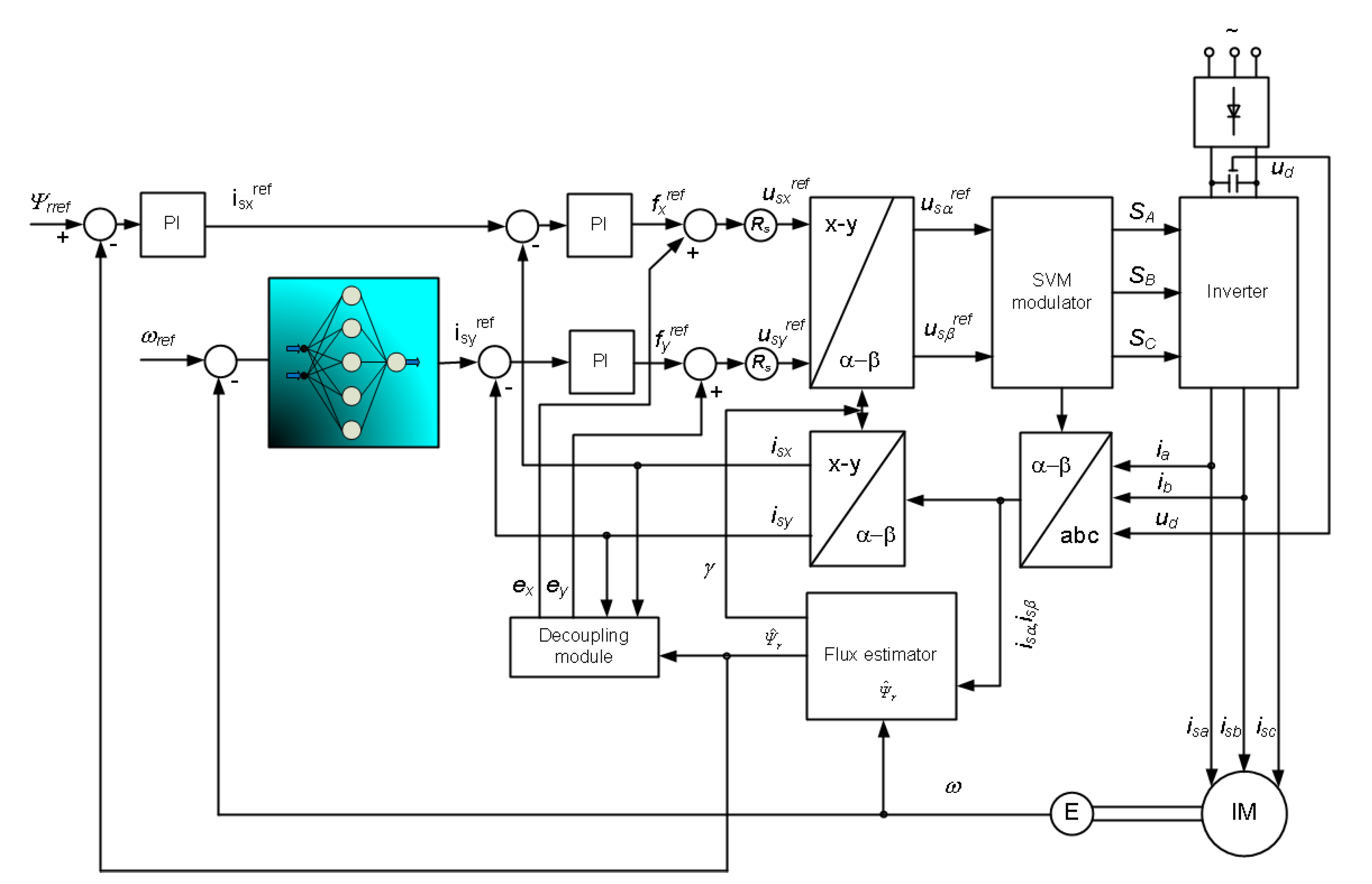
Figure 1. The Direct Field Oriented Control with neural speed controller.
Energies 13 06541 g001
Figure 2. The scheme of adaptive control structure.
Energies 13 06541 g002
Figure 3. Results of data processing in optimization process—initial and final results (a), transients of speed in selected steps (b), changes in wolf population in searching for kp (c), changes in wolf population in searching for ki (d), and fluctuation of optimized parameters (e).
Energies 13 06541 g003aEnergies 13 06541 g003b
Figure 4. Results of optimization—speed signals and cost function—performed for different conditions: using Equation (45) as a cost function (a), with input filter (b), with noise in speed signal (c), and with Formula (60) applied as objective function definition (d).
Energies 13 06541 g004aEnergies 13 06541 g004b
Figure 5. Results of the controller parameter optimization—influence of the initial value selection.
Energies 13 06541 g005aEnergies 13 06541 g005b
Figure 6. Transients of state variables (speed ω (ad) and current isy (e,f)) in the Direct Field Oriented Control structure with neural speed controller—nominal values of parameters.
Energies 13 06541 g006
Figure 7. Transients of state variables (speed ω and current isy) in the Direct Field Oriented Control structure with neural speed controller - changes in the mechanical time constant: tm = 2tmn (ac); tm = 0.5tmn (df).
Energies 13 06541 g007
Figure 8. Transients of motor speed—influence of initial weight randomization (ac) and influence of learning coefficient (df).
Energies 13 06541 g008aEnergies 13 06541 g008b
Figure 9. Elements of laboratory equipment.
Energies 13 06541 g009
Figure 10. Transients of state variables—speed (ad), component of current (e) and hodograph of the rotor flux vector (f) observed in the DFOC structure with PI speed controller with neural compensation.
Energies 13 06541 g010
Figure 11. Transients of state variables—speed (ad), component of current (e) and hodograph of the rotor flux vector (f) observed in the DFOC structure with PI speed controller with neural compensation: load switching.
Energies 13 06541 g011aEnergies 13 06541 g011b
Figure 12. Transients of speed (ad) measured in the DFOC structure with PI speed controller and the RBFNN compensation—influence of initial weight randomization (comparison).
Energies 13 06541 g012
Figure 13. Transients of state variables—speed (ac) and component of current (df) measured in the DFOC structure with PI speed controller and neural compensation: influence of training coefficient.
Energies 13 06541 g013
Table 1. The influence of the initial value selection on the final optimization results.
Number of TestBefore OptimizationAfter Optimization
kp_initki_initkpki
Test 10.47260.43285.587261.9276
Test 24.66316.13575.594361.9402
Test 369.978060.00845.571561.7623
Table 2. Selected parameters of the control system.
ElementParameterValue
Induction motorNominal power1.1 kW
Voltage230 V
Current2.9 A
cos ϕ0.76
Torque7.6 Nm
Stator flux0.9809 Wb
Efficiency76%
Rotor speed1380 rpm
Frequency50 Hz
Moment of inertia0.002655 kgm2
Stator resistance5.9 Ω
Rotor resistance4.559 Ω
Magnetizing impedance392.5 mH
Stator leakage impedance24.8 mH
Rotor leakage impedance24.8 mH
GWO algorithmSize of population20
Number of iterations30
Total time of calculations159.5262 s
PI controllerkp5.5892
ki61.4973
RBFNN compensatorNumber of hidden nodes5
Range of training coefficientη ∈ <0.005; 0.1>
Initial weightsRandom numbers
Publisher’s Note: MDPI stays neutral with regard to jurisdictional claims in published maps and institutional affiliations.