Abstract
Distributed energy resource (DER) has been widely deployed, and distributed generation (DG) can complement the distribution system. Favorable DG deployment provides the grid-connected microgrid (MG) with stable voltage and reduces emission and power generation costs. DGs are considered distributed feeders, and MG is required to be operated under the optimal state. Reconfiguration is a practical approach to optimizing resource allocation. The optimal global solution is obtained via optimization algorithms. In this paper, three objectives are defined, namely, minimization of economic cost (ECC), emission cost (EMC), and voltage deviation (VD). Consequently, a fuzzy moth-flame optimization (FMFO) algorithm is proposed to coordinate the interests of multiple objectives. Moreover, the simulation is conducted based on the standard IEEE 33-bus radial distribution system (RDS), under which the impact of deployment of various DG type and quantity on the MG is explored. In particular, diverse DG combinations are tried under the increasing power demand, and a high-stable voltage strategy is proposed to meet the specific demands. The simulation results reveal that: (1) the DG type has a significant impact on ECC and EMC; (2) penetration level of DG shows a positive-like relationship with the MG stability; and (3) the proposed FMFO algorithm exhibits an efficient performance in convergence.
1. Introduction
Energy plays a vital role in social development. The massive consumption of traditional energy resources, represented by fossil fuels, has given rise to multiple problems, such as climate change [1] and environmental pollution [2]. With the rapid development of distributed energy resource (DER) technology, the demand for DER is also increasing dynamically, promoting profound changes in planning, configuration, operation, and control of the power system. Currently, DERs are accepted and deployed near houses as a part of the local power supply. A DER is a small-scale energy resource, making the traditional power generation mode undergo a significant transformation. In the traditional operation model, power is supplied by one or more centralized large-scale power plants, which provide power for long-distance loads through high-voltage transmission lines. The DER generation units, also called distributed generations (DGs), are integrated into the power network to provide power compensation for the power system [3]. The DER consists of controllable units (e.g., diesel engine (DE), microturbine (MT), and fuel cell (FC)) and uncontrollable units (e.g., wind turbine (WT) and photovoltaic (PV) cell) [4]. It is more flexible and faster to deploy the DGs compare with traditional power generators. Moreover, DGs’ deployment can bring higher reliability to the power system, provide higher power quality to the loads, reduce transmission loss in the distribution system, decrease power generation cost, and limit environmental pollution.
As the power system is deepening reform, traditional power systems are developing into smart grids (SGs). Microgrids (MGs) are considered cost-effective, environment-friendly, and user-satisfied solutions to the SG. The MG is a small-scale power generation and distribution system, which generally includes multiple components such as power converters (PCs), energy storage systems (ESSs), transformers, switchgears, transmission lines, and power consumers (loads) [5]. There are two operation modes of MG: grid-connected mode and islanded mode [6], respectively. However, considering unpredictable changes in the MG (such as transmission line failures, considerable fluctuations in loads, or DG faults) and the power distribution system’s economic and environmental factors, a practical solution is conducting MG reconfiguration [7]. The MG reconfiguration improves the system reliability, reduces the power generation cost, limits the emission pollution, reduces the power transmission loss (PTL), and stabilizes the voltage deviation (VD) in MGs, keeping the MG operated under the optimal state.
Various management strategies, control technologies, and optimization methods related to MG have emerged in recent years to provide reliable technical support for MGs. In [8], the progress of intelligent distribution technology is reviewed concisely, and the emerging technology and future development trend are determined to support the active management of the distribution network. Different MG frameworks are proposed in [9,10,11,12] to support energy management, power distribution, DG placement, and renewable energy sources. Hierarchical structures of MG control methods are introduced in [13,14,15,16,17] to handle the system control, energy storage, power distribution, and market behaviors.
Investigation and study on MG reconfiguration are not sufficient [18] and still facing numerous critical challenges. The MG reconfiguration is regarded as a multiobjective optimization process that requires the high performance of optimization algorithms. Considering DG deployment, [19,20,21] conducted the reconfiguration of the power systems to reduce PTL by applying novel optimization methods. Novel intelligent algorithms [22,23,24,25] are springing out to provide options to the optimization problems. The intelligent algorithms are high-efficient in solving single-objective optimization problems but mostly cannot independently deal with multiobjective optimization problems. [26,27,28,29,30] proposed hybrid methods, which combined conventional optimization algorithms with multiobjective approaches, such as stochastic method, Pareto dominance method, and fuzzy decision-making theory, to provide opportunities for multiobjective optimization solutions.
The construction of the power system infrastructure is a significant issue related to the livelihood of people. As the future of the power system, the MG presents an evident value in research and application. In the present studies, the research on multiobjective optimization algorithms is not sufficient; and few works have explored the impact of DG deployment on optimizing the MG system, especially on DG deployment strategies under increasing power demand.
This paper focuses on obtaining and analyzing the optimal solution for reconfigurable MGs. Three objectives: minimization of economic cost (ECC), minimization of emission cost (EMC), and minimization of voltage deviation (VD) are defined to describe multiple requirements of the MG, and a multiobjective optimization algorithm is in need for coordinating the global interests of multiple objectives. To supplement the shortcomings of the existing multiobjective optimization solutions, a novel FMFO algorithm, hybridized the nature-inspired Moth-flame optimizer (MFO) and heuristic fuzzy method, is proposed to solve the multiobjective problem defined in this paper. While considering the integration of MG and DG, the deployment strategy is crucial to achieving the MG voltage stability, especially in the high-stable VD required scenarios. Thus, the analysis and comparison of diverse DG combinations are necessary for developing the DG deployment strategy. Furthermore, the employment of three types of controllable DER generation units, DE, MT, and FC, are considered to explore the impact of diverse DG combinations on optimal reconfiguration results, such as the effect on load demand, bus voltage, and branch line current.
The main contributions of this paper are:
- Uncontrollable DER generation units, DE, MT, and FC, are studied, and the corresponding models of ECC, EMC, and VD are established in mathematical expression patterns, respectively;
- An FMFO algorithm is proposed to solve the multiobjective optimization problem and acquire the optimal global solution in MG reconfiguration;
- An in-depth exploration of the potential impact of DG type and quantity on the power distribution system’s performance is conducted by employing of penetration level of DG;
- The step-by-step changing power demands of prosumers are considered to study the optimization strategy under critical situations;
- A method to realize the high-stable voltage was studied that can provide a DG selection strategy for those who require high-quality power.
The remaining parts of this paper are organized as follows: Section 2 introduces the formation of mathematical models, including all relevant objective functions and the corresponding constraints. Section 3 presents the primary research process and the proposed hybrid optimization algorithm. Section 4 describes several related cases and scenarios, and the results obtained in the cases are analyzed. Finally, Section 5 gives a conclusion to this paper.
2. Problem Formulation
2.1. Objective Functions
Three objectives, minimization of ECC, minimization of EMC, and minimization of VD, are defined based on the desired changes in the MG. The relevant objective functions can be optimized through the novel intelligent algorithms while conducting system reconfiguration, and the mathematical models for the three objectives are established.
2.1.1. Minimization of ECC
In the test system of this paper, there are two primary sources of the power supply: one is from the utility grid (substation), and the other is from DER generation units (DGs). In this case, the total power generation cost can only be produced by these two types of energy supply. It should be equal to the sum of DGs’ generation cost and the utility grid’s generation cost. Due to the commercial nature of power generation, the power generation cost is considered the ECC. Therefore, the total ECC can be defined as:
where is the total ECC, , , , and represent the ECC caused by utility grid, DE, MT, and FC, respectively. Furthermore, the can be calculated as:
where is the active power supplied from the utility grid, and is the coefficient for calculating the ECC of the utility grid. For the DGs, the calculation of the ECC depends on the type and quantity of DGs. This paper defines that the three types of DGs are DE, MT, and FC, respectively. The ECC of DE is expressed as:
where is the active power generated by the i-th DE, is the DE quantity, and are the coefficients of the ECC of DE. Similarly, the ECC of MT is expressed as:
where is the active power generated by the j-th MT, is MT quantity, is the price of the natural gas, is the operation efficiency of the j-th MT, and is the low-hot value of natural gas. The subsequent ECC of FC is expressed as:
where is the power generated by the k-th FC, is the FC quantity, and is the operation efficiency of the k-th FC.
2.1.2. Minimization of EMC
The power generation may lead to varying degrees of environmental pollution according to the variety of power resources. Among the substances emitted, , and are considered to be the chief components that are the culprit for causing damage to the environment. For quantifying the degree of emissions, the EMC function is established as follows:
where is the total EMC, , , , and are the EMC of the utility grid, DE, MT, and FC, respectively. , , and represent the active power generated by the i-th DE, the j-th MT, and the k-th FC, respectively.
2.1.3. Minimization of VD
Voltage stability is a crucial index to reflect power quality. Controlling the bus VD within the tolerable range plays an essential role in improving the reliability of the distribution system [31]. VD refers to the difference between the real-time voltage and the reference voltage of all load buses, which can be expressed as:
where is the voltage of the i-th bus, is the reference voltage, and is the number of load buses.
2.2. Constraints
When reconfiguring the MG, all possibilities should be considered to set the necessary constraints to meet the actual situation. According to the characteristics, this work divides the constraints into equality constraints and inequality constraints.
2.2.1. Equality Constraint
In this work, equation constraints are mainly discussing the power balance in the distribution system, and the total input power should be equal to the sum of all loads and transmission loss. The power balance formula is as follows:
where , , , and are the active power generated by the grid, DE, MT, and FC, respectively. , , , and stand for the reactive power generated by the grid, DE, MT, and FC, respectively. and are the active and reactive power losses, and are active and reactive load demands.
2.2.2. Inequality Constraint
Inequality constraints are a set of conditional constraints that consider all possibilities (such as the boundaries of variables) and can only be expressed with inequalities. Constraints on power generation operation:
where is the current output power, and is the previous output power, is the up-ramp limit of the i-th generator (MW/time-period), and is the down-ramp limit of the i-th generator (MW/time-period). Due to the physical characteristics of power equipment, the constraints of line flows are:
where is the number of generator buses, and is the number of line branches.
The constraints of DG Power factor:
Each kind of dispatchable DG’s power handling capacity is limited because of its current and voltage control loops. Therefore, in any case, the power and generated by DG follow the droop relationship:
The constraints of minimum in-service and out-service time:
The constraints of storage battery:
3. Hybrid FMFO Algorithm
Intelligent optimization algorithms with reliable performance and fast convergence came into being and have impressed many researchers and are successfully applied in many fields. Compared with traditional algorithms, intelligent optimization algorithms have many advantages and higher efficiency in optimizing nonlinear or multi-extreme complex functions. For acquiring the optimal DG placement in the reconfigurable MGs, this paper proposes a hybrid multiobjective optimization algorithm which applied the fuzzy method to the MFO algorithm.
3.1. MFO Algorithm
The MFO algorithm [25] is a novel nature-inspired algorithm first proposed by Seyedali Mirjalili in 2015. The algorithm sets a fixed number of moths to wander in the variable space to search for the flame, the optimal solution of the objective function. The execution process of the MFO algorithm is summarized and described in Algorithm 1.
| Algorithm 1 MFO Algorithm |
 |
3.2. Heuristic Fuzzy
The MG optimization involves three objectives: minimization of ECC, EMC, and VD. The scheme of heuristic fuzzy combined with the MFO algorithm is proposed to balance the benefit of multiple objectives. The fuzzy membership functions are employed for each objective function with upper and lower limits to enjoy high flexibility for making decisions. The developed membership functions can be modified to change the contribution of each objective function of the problem based on their requirements. The objective functions involved are described in detail below.
3.2.1. Membership Function for ECC
The total power generation cost of the solution should be minimized. Therefore, for a given load level , the ratio of the total power generation cost before and after optimization of the distribution system is defined as follows:
In the equation, for lower values, the solution can get more benefits. The membership function corresponding to minimization is expressed as:
In this work, and equal to 0.5 and 1, respectively. The value of refers to the minimum acceptable amount of saving to 50%.
3.2.2. Membership Function for EMC
The same as , the EMC should be minimized, and the is defined as follows:
The membership function corresponding to the minimization of is expressed as,
where and are equal to 0.5 and 1, respectively. The value refers to the minimum acceptable amount of saving to 50%.
3.2.3. Membership Function for VD
Among the power flow constraints, bus voltage constraints are more sensitive when external equipment is connected to the system. Therefore, minimization of VD was considered as one of the objectives, along with the reduction of total PTL. The minimum bus voltage (MBV) of the system was obtained from the load flow equation for each new population of MFO. This membership function determines the deviation of the of the new population () to the initial (). The membership function for the population can be expressed as follows:
where and are considered as 0.05 and 0.1, respectively. The reflects the maximum voltage of network buses is <1.05 (or the minimum voltage of network buses is >0.95), then . The value of is calculated and expressed below:
From the Equations (28), (30), and (31), the fuzzified values for the , , and can be obtained as , , and , respectively. In order to obtain a compromise solution among these three fuzzified values, the fuzzy decision set is introduced, which is expressed as
The equation is considered as the fitness function for the MFO algorithm. As a result, each population of the MFO produces a compromised solution among the three objective functions.
4. Simulation and Discussion
The simulations are prepared in a desktop computer installed with Microsoft Windows 10 Enterprise Edition as the operating system for coding and testing. The CPU of the computer is Intel Core (TM) i5-4660, equipped with an 8G Samsung DDR3-1600 as the memory. In terms of software, the Java NetBeans IDE 7.2 is adopted as a development tool to simulate the standard IEEE 33-bus RDS, which integrated with MGs deployed according to the loops. Figure 1 shows the schematic diagram of the test system. Since there are five loops in the standard IEEE 33-bus RDS, the test system maximizes the deployment of the hypothetical MGs in these loops to ensure that the MGs can generally work in the grid-connected mode and are also able to operate in the islanded mode under the specific conditions [32].
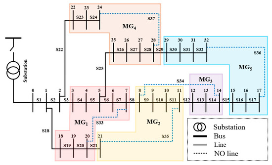
Figure 1.
A single-line diagram of standard IEEE 33-bus radial distribution system (RDS).
The primary purpose of the simulation is to obtain the optimal global solution for optimization and explore the optimal DG placement strategy. For evaluating the performance of the FMFO algorithm, the simulations are conducted for the case study, and numerous results are gathered for analysis.
4.1. Initialization and Settings
In the standard IEEE 33-bus RDS, the initial basic kV and MVA of the test system are set to 12.66 kV and 100 MVA, and the basic active power and reactive power demands are 3.715 MW and 2.3 MVAR, respectively. For facilitating the research, the simulations take the basic load as a reference. It assumes that the MBV limit is 0.9 per unit (pu) and that each line has a maximum branch current capacity of 400 A (excluding lines connected to the feeder). There are 33 buses in the test system (from 0 to 32). In the initial state, the normally open (NO) switches are S33, S34, S35, S36, and S37, and the normally closed (NC) switches are from S1 to S32. Table 1 shows the initial state of the lines and buses in the test system.

Table 1.
The initial state of the distribution test system.
This investigation divides the primary parameters or variables involved in the optimization process into two categories: one is called generation-parameter, which plays a crucial role in energy generation, and the values can be collected from the corresponding objective models. Another category is named optimization-variable, which plays a decisive role in the simulation results, and the values are the optimal locations of DGs and the open switches. Table 2 and Table 3 list the primary generation-parameters and corresponding values in our simulation.
Table 2.
Primary parameters of economic cost (ECC) models [33].
Table 3.
Emission coefficients related to grid and distributed energy resources (DERs) [34,35].
According to the characteristics, this study further divides the optimization-variable into the location-optimization variable, type-optimization variable, and quantity-optimization variable. The location-optimization variables refer to the locations of the switches and DGs, the type-optimization variables describe the types of DGs, and the quantity-optimization variables define the number of active DGs. The simulations also restricted each MG to one open switch to keep the radial structure. By changing the location of the open switches, the topology of the power distribution system is changed. Table 4 lists the boundaries of the location-optimization variable values.
Table 4.
Boundaries of location-optimization variable values.
4.2. Simulation and Case Study
Simulations are conducted in the test system, which has integrated the standard IEEE 33-bus RDS and five MGs. For exploring the optimal DG placement strategy, DE, MT, and FC are deployed with holistic consideration of the ECC, EMC, MBV, and PTL. It is assumed that all DGs operate at rated power, where the rated power of DE, MT, and FC are set to 0.4 MW/h, 0.6 MW/h, and 0.5 MW/h, respectively. Then, the changes of crucial parameters in reconfiguration were analyzed, and the obtained performance feedback is discussed from the perspective of multiple DG combinations. Through analyzing the results, the changes and their trends can be found to assist in formulating the DG placement strategy in different cases.
4.2.1. Case 1: Simple DG Deployment
In this phase, the number of DE, MT, and FC deployed in the test system is restricted to 1, but the types of DGs are not limited in simulation. The results of system reconfiguration shown in Table 5 are effectively obtained due to the low computational complexity. For better comparing the changes brought by reconfiguration after deploying DG(s), a simulation without DG deployment is conducted as a reference. The open switches were changed to the optimal locations after reconfiguration.
Table 5.
Reconfiguration results for single DG and corresponding combinations.
Since a DE deployed in the MGs, the EMC, MBV, and PTL are improved in evidence, while ECC is increased on the contrary due to the higher generation cost of DE. However, Table 5 discloses the apparent improvements in all aspects if any MG is deployed with an MT or FC. The ECC, EMC, and PTL were efficiently reduced, the MBV is significantly optimized, and the MBV trended to be more stable with the increasing usage of DGs. Different types of DG bring different changes to MG, which is closely related to their physical and electrical characteristics. Due to the ECC, DE has a negative contribution to reducing ECC. Therefore, the ECC of DG should be fully considered in the selection of MG before the deployment of DG. Compared with DE, FC and MT play a positive role in ECC and EMC, which can be considered while selecting DGs.
4.2.2. Case 2: Effect of DG Quantity
Most of the changes caused by DG deployment are positive, but the qualitative or quantitative measurement of the impact of DG type and quantity on the test system is still an issue. To make up for the deficiencies, Case 2 gradually increased the number of different types of DG from 1 to maximum and monitored the changes in system parameters. It is assumed that the DGs deployed in the test system are active and running at the rated power. Owing to the limitation of the total load demand, DGs cannot be deployed endlessly. According to the generation capacity of different DG types, the total DG generation should be less than or equal to the sum of load demands and line transmission losses. The maximum number of DE, MT, and FC are restricted to 9, 6, and 7, respectively. Moreover, the penetration level (PL) [36] of DG is employed to measure the impact of DG deployment on MG optimization. The PL of DGs is calculated as:
In this phase, the simulation is carried out for probing the impact of increasing DG number on total ECC. Figure 2 shows the impact on ECC, EMC, MBV, and PTL in reconfiguration by increasing DE, MT, and FC quantity, limiting the maximum number of DG to 6 for comparison. Figure 2a indicates that the increase of DE has the opposite effect on reducing ECC, while with the increase in the number of MT and FC, the total ECC shows a linear-like slow downward trend. In the aspect of EMC shown in Figure 2b, with the increase of three types of DG, the EMC reduced in varying degrees, and the performance of FC is outstanding, followed by MT, and the improvement of DE is the lowest. In terms of voltage stability, it can be found in Figure 2c that there is a significant correlation between EMC and DG rated power. Finally, in terms of line transmission loss, pointed in Figure 2d, various types of DGs brought varying degrees of improvement, with FC still performs best among the three types.
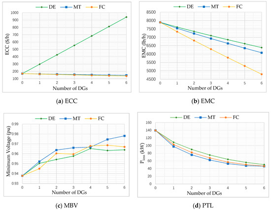
Figure 2.
ECC, emission cost (EMC), minimum bus voltage (MBV), and power transmission loss (PTL) changing curve with the increasing number of DGs.
The utilize of PL quantified the impact of DG with different generation capacities on the MG system targets and lessened the difference caused by distinct DG rated power. From the perspective of DG PL, as shown in Table 6, Table 7 and Table 8, the increasing number of DE, MT, and FC leads to an increase in DG penetration levels. In contrast, ECC, EMC, PTL, and MBV all show divergent trends and degrees on the change. Moreover, the increase of PL makes DG play a more significant role in MGs and profoundly impacts the optimal fitness values of essential objectives and the MG configurations.
Table 6.
Reconfiguration results of the increasing diesel engine (DE) deployment.
Table 7.
Reconfiguration results of the increasing microturbine (MT) deployment.
Table 8.
Reconfiguration results of the increasing MT deployment.
The highest PL of DE, MT, and FC in tables are 94.64%, 94.56%, and 92.01%. Comparing the corresponding results of the maximum PL, the FC manifests the overall advantages over the other two types of DGs: the lower ECC, fewer EMC, less PTL, and more stable bus voltage.
4.2.3. Case 3: Diverse DG Combinations
This phase fixed the DG quantity to 5 in the simulation, based on which diverse combinations of DE, MT, and FC are considered to study the potential impact in system optimization on the essential parameters. Moreover, both manual mode and automatic mode are implemented while coding, where the manual mode is to simulate system reconfiguration in the case of specified DG type and quantity. In contrast, the automatic mode can automatically choose an optimal combination for system reconfiguration according to the given DG quantity. As listed in Table 9, the reconfiguration results of six given combinations and an auto-select combination show some different performance between two modes and all combinations. On account of the significant advantages of FC presented in Section 4.2.2, the automatic mode tends to consider the high performance of FC and the generation capacity of MT in choosing DGs, thus obtaining better configuration than the other six fixed combinations in terms of synthesis.
Table 9.
Reconfiguration results under various combinations of 5 DGs.
4.2.4. Case 4: Under Changing Power Demand
Power demand is usually not fixed but continually changing. MGs need to deal with sudden high-power demand, so it is necessary to consider the DG placement and system reconfiguration under various complicated conditions. Based on the forecasts of power demand and consumption in [37], this phase adjusted each bus’s energy demand within an acceptable range to imitate the changes in real power demands. For investigating the significance of system reconfiguration and DG placement under the changing power demand, the simulation increases the total power demand from 100% of the reference power demand to 200%, by 10% for each step.
Moreover, the simulation performed three scenarios based on the changing power demands (shown in Table 10). Scenario 1 simulates with a fixed DG combination, in which the number of DE, MT, and FC are set to 2 separately. Scenario 2 conducted an auto-select mode and set the DG quantity to 6, which decided the six FCs as the optimal combination. For obtaining more results, this simulation maximizes the deployment of DGs in Scenario 3 and lets the proposed strategy decide the DG quantity and the optimal DG combination. The comparison of the scenarios is shown in Figure 3.
Table 10.
The changing power demands of all buses from 100% to 200%.
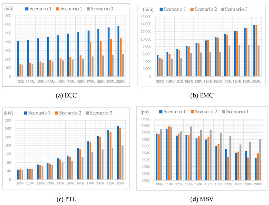
Figure 3.
Comparison of ECC, EMC, PTL, and MBV under changing power demand in three scenarios.
The results obtained in the three scenarios are shown in Table 11, Table 12 and Table 13. It is significant that with the increase of power demand from reference quantity to 200%, the total ECC, total EMC, and PTL in the three scenarios increase to varying degrees; only the voltage stability shows a fluctuating decrease. Scenario 2 shows more significant advantages from a scenario perspective than Scenario 1 in terms of ECC and EMC. In terms of PTL and voltage stability, Scenario 2 performs slightly better than Scenario 1 in the reference power demand’s vicinity. As the power demand increases to 200%, the PTL and MBV of Scenario 2 are getting higher than those in Scenario 1. Scenario 3 performs significantly better than Scenario 1 and Scenario 2 in EMC, ECC, PTL, and voltage stability. Moreover, as power demand increases, this advantage becomes more apparent.
Table 11.
Scenario 1: system reconfiguration results of DG combinations under 6 DGs and increasing power demand.
Table 12.
Scenario 2: system reconfiguration results of auto-select DG combination under 6 DGs and increasing power demand.
Table 13.
Scenario 3: system reconfiguration results of auto-select DG combination under maximum DG quantity and increasing power demand.
4.3. Analysis and Discussion
The significance of MG optimization is to achieve the optimal allocation of resources. DER plays a prominent role in regulating the peak energy demands, considering both economic and environmental protection. Deploying DGs in the reconfiguration of MG can solve many problems encountered in the development of SG.
4.3.1. Evaluation of Algorithm
This paper proposed an FMFO algorithm to solve the multiobjective issue. As shown in Figure 4, the improvement of system optimization by employing the FMFO algorithm is evident in the bus voltage and line current in MGs. The MBV was improved to 0.9378 (pu) after system reconfiguration without deploying DG. While deploying a DE, the MBV has reached 0.9503 (pu), even reached 0.9661 (pu) while deploying a simple DG combination. Simultaneously, the line current is optimized with the appropriate utilization of DG(s) or DG combination; each line’s current is significantly decreased.
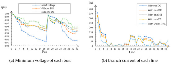
Figure 4.
Effect of DG deployment on bus voltage and line current of system reconfiguration.
In order to reflect the convergence of the proposed algorithm, our simulation randomly selected ten results in the case of without DG deployment, with DE deployment, with MT deployment, and with FC deployment, respectively. Figure 5 shows the convergence of the proposed algorithm on ECC that the optimal solutions are obtained within a maximum of 20 iterations without DG deployment and within 44 iterations among the 30 runs while DG is deployed. Moreover, a fuzzy genetic algorithm (FGA) and fuzzy particle swarm optimization (FPSO) are implemented in the simulation to compare the convergence with the proposed FMFO on the PTL. As shown in Figure 6, 20 runs of FGA, FPSO, and FMFO are conducted separately to calculate the average PTL. The proposed FMFO algorithm shows advantages in both simulations deployed without DG and deployed with an MT. In the simulations without DG deployed, the FMFO, FPSO, and FGA obtained the optimal solutions at the average iteration numbers of 9.7, 14.9, and 34.2, respectively; and in the simulations with an MT deployed, the FMFO, FPSO, and FGA obtained the optimal solutions at the average iteration numbers of 13.6, 18.5, and 46.3, respectively.
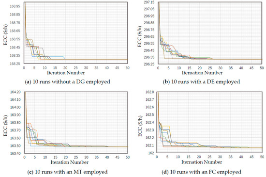
Figure 5.
The convergence of the proposed algorithm on ECC.
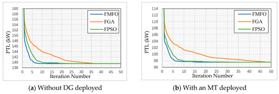
Figure 6.
Comparison of convergence of fuzzy genetic algorithm (FGA), fuzzy particle swarm optimization (FPSO), and fuzzy moth-flame optimization (FMFO) on power transmission loss (PTL).
The effect of the DG penetration level on improving PTL is usually positive [36]. As shown in Table 14, this simulation obtained better results in which the PTL is 62.18 kW under the auto-select mode, in the case where the DG penetration level was 47.65%. Compared with the optimal results in [38], the PTL obtained in this paper was reduced by 7.35%; meanwhile, the MBV was still kept at a considerable level.
Table 14.
Comparison of reconfiguration results under the deployment of 3 DGs.
4.3.2. Data Analysis and DG Placement Strategy
The deployment of DG(s) leads to a significant impact on MG optimization, as shown in Table 5. Compared with no DG deployed, employing a DE has increased the ECC from $169.6002/h to $297.4400/h by 75.38%. In contrast, the deployment of an MT and FC have decreased the corresponding ECC by 2.98% and 3.80%. In terms of EMC, the applying of a DE, MT, and FC has reduced the total EMC from 7982.8072 lb/h to 7608.5086 lb/h, 7536.1043 lb/h, and 7332.4768 lb/h by 3.60%, 4.52%, and 7.10%, respectively. Similarly, by applying a DE, MT, and FC, the PTL decreased by 22.15%, 30.09%, and 26.43%, and the MBV increased from 0.9378 pu to 0.9503 pu, 0.9522 pu, and 0.9450 pu, respectively. When DE, MT, and FC are combined, the effects of different DGs on system optimization are superimposed.
Through analyzing the impact of DG type on system optimization and the superposition effect of DG quantity, the simulation results where DG quantity increases from 1 to the maximum are shown in Table 6, Table 7 and Table 8. In corresponding Figure 2, Figure 3 and Figure 4, the ECC curves and EMC curves present a quasi-linear decrease with the increase of DG quantity except for DE; meanwhile, the PTL shows an exponent-like reduction, and the MBV shows an irregular improvement. The changing trends of ECC and EMC rely mainly on the characteristics of DGs.
As further exploring the reconfiguration under diverse DG combinations, Table 9 shows that the EMC, ECC, PTL, and the MBV improved to varying degrees under various DG combinations. Compared with Table 5, the MBV is more stable, illustrating the importance of DG quantity increment to voltage stability. However, it is worth noticing that the MBV value of auto-select mode is high, reaching 0.9739 pu, due to its higher DG penetration level among all DG combinations. From the perspective of MBV stability, the performance of an appropriate multitype DG combination is slightly better than that of the optimal single-type DG combination in case that the DG quantity is fixed.
Thus, if the high voltage stability is required, it is needed to maximize the utilization of DGs, and then choose the appropriate multitype DG combination to meet the different power replenishment needs of buses.
Compare Table 11 with Table 12, when the power demand increases from 100% to 200%, the PTL and MBV of the combination with two DEs, two MTs, and two FCs are 252.1833 kW and 0.9325 pu; the combination of auto-select mode are 243.3098 kW and 0.9396 pu. The optimal DG combination showed more considerable advantages in PTL and MBV with increased power demand. Nevertheless, the ECC and EMC of auto-select mode are $447.5775/h and 13,709.5232 lb/h that is much better than that of the fixed 6 DGs $580.3721/h and 13,777.4195 lb/h. With the increase of power demand in the distribution system, the fixed DG quantity makes the penetration level decreased. Table 13 shows relatively stable DG penetration levels by maximizing DGs’ deployment under the auto-select mode. Compared with Table 11 and Table 12, the ECC, EMC, PTL, and MBV in Table 13 are comprehensively improved due to the higher DG penetration level. The ECC, EMC, PTL, and MBV have also been improved to $261.6486/h, 8267.5435 lb/h, 159.0155 kW, and 0.9607 pu under the 200% power demand.
As a result of the bus voltage’s reliable stability in the simulation, the FMFO algorithm paid more attention to energy saving and emission reduction while ensuring high-quality power supplying. Maximizing the DG penetration level can effectively optimize the power distribution system’s output, but the appropriate DG combination is necessary to improve system parameters further. The fundamental cause is that making the current average and at a lower level will stable the bus voltage and minimize the energy transmission loss.
5. Conclusions
This paper conducted the system optimization of MGs based on the standard IEEE 33-bus RDS and proposed an FMFO algorithm to solve the multiobjective optimization problem. The proposed FMFO algorithm showed an efficient performance on convergence comparing with classical FGA and FPSO. The obtained optimal solution via MG reconfiguration has considered integrating with DGs and achieved minimum PTL, ECC, EMC, and VD comparing with existing research. Moreover, our simulations have considered various DG combinations to explore the effect of DG type and quantity on MG reconfiguration results. Furthermore, we have investigated the results in four step-by-step cases and gained the optimal solution for each. The optimal DG placement and combination were explored under the increasing power demand, which formed a DG deployment strategy for decision-making. The simulation results reveal that: the proposed FMFO algorithm is a reliable supplement for multiobjective optimization approaches in MG reconfiguration; it requires fewer iterations to obtain the optimal solution than other optimizers; appropriate DG selection and deployment strategy is conducive to obtaining the optimal global solution, especially under the critical power demand conditions.
Author Contributions
Conceptualization, X.W. and I.-h.R.; methodology, T.S. and H.K.; investigation, X.W. and T.S.; writing—original draft preparation, X.W.; writing—review and editing, T.S. and H.K.; funding acquisition: I.-h.R. All authors have read and agreed to the published version of the manuscript.
Funding
This research received no external funding.
Acknowledgments
This work was supported by the Institute for Information and Communications Technology Promotion (IITP) grant funded by the Korea government (MSIT) (No. 2018-0-00508), Development of blockchain-based embedded devices and platform for MG security and operational efficiency. This work was supported in part by the Human Resources Development Program (Grant No. 20194010201800) of the Korea Institute of Energy Technology Evaluation and Planning (KETEP) grants funded by the Korean government (Ministry of Trade, Industry, and Energy).
Conflicts of Interest
The authors declare no conflict of interest.
Abbreviations
The following abbreviations are used in this manuscript:
| DE | Diesel engine |
| DER | Distributed energy resource |
| DG | Distributed generation |
| ECC | Economic cost |
| EMC | Emission cost |
| ESS | Energy storage systems |
| FC | Fuel cell |
| FMFO | Fuzzy moth-flame optimization |
| MG | microgrid |
| MT | microturbine |
| MBV | Minimum bus voltage |
| MFO | Moth-flame optimizer |
| NC | normally closed |
| NO | normally open |
| PL | Penetration level |
| PV | photovoltaic |
| PC | Power converter |
| PTL | Power transmission loss |
| RDS | Radial distribution system |
| SG | Smart grid |
| VD | Voltage deviation |
| WT | Wind turbine |
References
- Höök, M.; Tang, X. Depletion of fossil fuels and anthropogenic climate change—A Review. Energy Policy 2013, 52, 797–809. [Google Scholar] [CrossRef]
- Withagen, C. Pollution and exhaustibility of fossil fuels. Resour. Energy Econ. 1994, 16, 235–242. [Google Scholar] [CrossRef]
- Singh, M.; Khadkikar, V.; Chandra, A.; Varma, R.K. Grid interconnection of renewable energy sources at the distribution level with power-quality improvement features. IEEE Trans. Power Deliv. 2011, 26, 307–315. [Google Scholar] [CrossRef]
- Li, Y.; Wang, P.; Gooi, H.B.; Ye, J.; Wu, L. Multi-Objective optimal dispatch of microgrid under uncertainties via interval optimization. IEEE Trans. Smart Grid 2019, 10, 2046–2058. [Google Scholar] [CrossRef]
- Meng, L.; Sanseverino, E.R.; Luna, A.; Dragicevic, T.; Vasquez, J.C.; Guerrero, J.M. Microgrid supervisory controllers and energy management systems: A Literature Review. Renew. Sustain. Energy Rev. 2016, 60, 1263–1273. [Google Scholar] [CrossRef]
- Parhizi, S.; Lotfi, H.; Khodaei, A.; Bahramirad, S. State of the art in research on microgrids: A Review. IEEE Access 2015, 3, 890–925. [Google Scholar] [CrossRef]
- Kavousi-Fard, A.; Khodaei, A.; Bahramirad, S. Improved efficiency, enhanced reliability and reduced cost: The transition from static microgrids to reconfigurable microgrids. Electr. J. 2016, 29, 22–27. [Google Scholar] [CrossRef]
- Zhao, J.; Wang, C.; Zhao, B.; Lin, F.; Zhou, Q.; Wang, Y. A review of active management for distribution networks: Current status and future development trends. Electr. Power Compon. Syst. 2014, 42, 280–293. [Google Scholar] [CrossRef]
- Niknam, T.; Kavousi-Fard, A. Optimal energy management of smart renewable micro-grids in the reconfigurable systems using adaptive harmony search algorithm. Int. J. Bio-Inspired Comput. 2016, 6, 184–194. [Google Scholar] [CrossRef]
- Gazijahani, F.S.; Salehi, J. Stochastic multi-objective framework for optimal dynamic planning of interconnected microgrids. IET Renew. Power Gener. 2017, 11, 1749–1759. [Google Scholar] [CrossRef]
- Wang, Z.; Chen, B.; Wang, J.; Kim, J.; Begovic, M.M. Robust optimization based optimal dg placement in microgrids. IEEE Trans. Smart Grid 2014, 5, 2173–2182. [Google Scholar] [CrossRef]
- Khorram-Nia, R.; Bahmani-Firouzi, B.; Simab, M. Optimal switching in reconfigurable microgrids considering electric vehicles and renewable energy sources. J. Renew. Sustain. Energy 2018, 10, 1–18. [Google Scholar] [CrossRef]
- Olivares, D.E.; Mehrizi-Sani, A.; Etemadi, A.H.; Cañizares, C.A.; Iravani, R.; Kazerani, M.; Hajimiragha, A.H.; Gomis-Bellmunt, O.; Saeedifard, M.; Palma-Behnke, R.; et al. Trends in microgrid control. IEEE Trans. Smart Grid 2014, 5, 1905–1919. [Google Scholar] [CrossRef]
- Wu, X.; Wang, X.; Qu, C. A Hierarchical framework for generation scheduling of microgrids. IEEE Trans. Power Deliv. 2014, 29, 2448–2457. [Google Scholar] [CrossRef]
- Palizban, O.; Kauhaniemi, K.; Guerrero, J.M. Microgrids in active network management—Part I: Hierarchical control, energy storage, virtual power plants, and market participation. Renew. Sustain. Energy Rev. 2014, 36, 428–439. [Google Scholar] [CrossRef]
- Bidram, A.; Davoudi, A. Hierarchical structure of microgrids control system. IEEE Trans. Smart Grid 2012, 3, 1963–1976. [Google Scholar] [CrossRef]
- Guerrero, J.M.; Vasquez, J.C.; Matas, J.; de Vicuna, L.G.; Castilla, M. Hierarchical control of droop-controlled AC and DC microgrids—A general approach toward standardization. IEEE Trans. Ind. Electron. 2011, 58, 158–172. [Google Scholar] [CrossRef]
- Shariatzadeh, F.; Vellaithurai, C.B.; Biswas, S.S.; Zamora, R.; Srivastava, A.K. Real-Time implementation of intelligent reconfiguration algorithm for microgrid. IEEE Trans. Sustain. Energy 2014, 5, 598–607. [Google Scholar] [CrossRef]
- Abd El-salam, M.F.; Beshr, E.; Eteiba, M.B. A new hybrid technique for minimizing power losses in a distribution system by optimal sizing and siting of distributed generators with network reconfiguration. Energies 2018, 11, 3351. [Google Scholar] [CrossRef]
- Badran, O.; Mekhilef, S.; Mokhlis, H.; Dahalan, W. Optimal reconfiguration of distribution system connected with distributed generations: A Review of different methodologies. Renew. Sustain. Energy Rev. 2017, 73, 854–867. [Google Scholar] [CrossRef]
- Jabbari-Sabet, R.; Moghaddas-Tafreshi, S.-M.; Mirhoseini, S.-S. Microgrid operation and management using probabilistic reconfiguration and unit commitment. Int. J. Electr. Power Energy Syst. 2016, 75, 328–336. [Google Scholar] [CrossRef]
- Eskandar, H.; Sadollah, A.; Bahreininejad, A.; Hamdi, M. Water cycle algorithm–A novel metaheuristic optimization method for solving constrained engineering optimization problems. Comput. Struct. 2012, 110–111, 151–166. [Google Scholar] [CrossRef]
- Mirjalili, S.; Lewis, A. The whale optimization algorithm. Adv. Eng. Softw. 2016, 95, 51–67. [Google Scholar] [CrossRef]
- Mirjalili, S. The ant lion optimizer. Adv. Eng. Softw. 2015, 83, 80–98. [Google Scholar] [CrossRef]
- Mirjalili, S. Moth-flame optimization algorithm: A novel nature-inspired heuristic paradigm. Knowl. Based Syst. 2015, 89, 228–249. [Google Scholar] [CrossRef]
- Sedighizadeh, M.; Bakhtiary, R. Optimal multi-objective reconfiguration and capacitor placement of distribution systems with the Hybrid Big Bang–Big Crunch algorithm in the fuzzy framework. Ain Shams Eng. J. 2016, 7, 113–129. [Google Scholar] [CrossRef]
- Jafari, A.; Ganjeh Ganjehlou, H.; Baghal Darbandi, F.; Mohammadi-Ivatloo, B.; Abapour, M. Dynamic and multi-objective reconfiguration of distribution network using a novel hybrid algorithm with parallel processing capability. Appl. Soft Comput. 2020, 90, 106146. [Google Scholar] [CrossRef]
- Chen, Q.; Wang, W.; Wang, H.; Wu, J.; Li, X.; Lan, J. A social beetle swarm algorithm based on grey target decision-making for a multi-objective distribution network reconfiguration considering partition of time intervals. IEEE Access 2020, 8, 204987–205013. [Google Scholar] [CrossRef]
- Souifi, H.; Kahouli, O.; Hadj Abdallah, H. Multi-objective distribution network reconfiguration optimization problem. Electr. Eng. 2019, 101, 45–55. [Google Scholar] [CrossRef]
- Kianmehr, E.; Nikkhah, S.; Rabiee, A. Multi-objective stochastic model for joint optimal allocation of DG units and network reconfiguration from DG owner’s and DisCo’s perspectives. Renew. Energy 2019, 132, 471–485. [Google Scholar] [CrossRef]
- Li, H.; Li, F.; Xu, Y.; Rizy, D.T.; Kueck, J.D. Adaptive voltage control with distributed energy resources: Algorithm, theoretical analysis, simulation, and field test verification. IEEE Trans. Power Syst. 2010, 25, 1638–1647. [Google Scholar] [CrossRef]
- Ganjian-Aboukheili, M.; Shahabi, M.; Shafiee, Q.; Guerrero, J.M. Seamless transition of microgrids operation from grid-connected to islanded mode. IEEE Trans. Smart Grid 2020, 11, 2106–2114. [Google Scholar] [CrossRef]
- Li, P.; Xu, D.; Zhou, Z.; Lee, W.-J.; Zhao, B. Stochastic optimal operation of microgrid based on chaotic binary particle swarm optimization. IEEE Trans. Smart Grid 2016, 7, 66–73. [Google Scholar] [CrossRef]
- El-Ela, A.A.A.; El-Sehiemy, R.A.; Abbas, A.S. Optimal placement and sizing of distributed generation and capacitor banks in distribution systems using water cycle algorithm. IEEE Syst. J. 2018, 12, 3629–3636. [Google Scholar] [CrossRef]
- Kefayat, M.; Lashkar Ara, A.; Nabavi Niaki, S.A. A hybrid of ant colony optimization and artificial bee colony algorithm for probabilistic optimal placement and sizing of distributed energy resources. Energy Convers. Manag. 2015, 92, 149–161. [Google Scholar] [CrossRef]
- Srivastava, A.K.; Kumar, A.A.; Schulz, N.N. Impact of distributed generations with energy storage devices on the electric grid. IEEE Syst. J. 2012, 6, 110–117. [Google Scholar] [CrossRef]
- Eseye, A.T.; Lehtonen, M.; Tukia, T.; Uimonen, S.; John Millar, R. Machine learning based integrated feature selection approach for improved electricity demand forecasting in decentralized energy systems. IEEE Access 2019, 7, 91463–91475. [Google Scholar] [CrossRef]
- Mohamed Imran, A.; Kowsalya, M.; Kothari, D.P. A novel integration technique for optimal network reconfiguration and distributed generation placement in power distribution networks. Int. J. Electr. Power Energy Syst. 2014, 63, 461–472. [Google Scholar] [CrossRef]
- Saonerkar, A.K.; Bagde, B.Y. Optimized DG placement in radial distribution system with reconfiguration and capacitor placement using genetic algorithm. In Proceedings of the 2014 IEEE International Conference on Advanced Communications, Control and Computing Technologies, Ramanathapuram, India, 8–10 May 2014; pp. 1077–1083. [Google Scholar]
- Rao, R.S.; Ravindra, K.; Satish, K.; Narasimham, S.V.L. Power loss minimization in distribution system using network reconfiguration in the presence of distributed generation. IEEE Trans. Power Syst. 2013, 28, 317–325. [Google Scholar] [CrossRef]
- Rajaram, R.; Sathish Kumar, K.; Rajasekar, N. Power system reconfiguration in a radial distribution network for reducing losses and to improve voltage profile using modified plant growth simulation algorithm with Distributed Generation (DG). Energy Rep. 2015, 1, 116–122. [Google Scholar] [CrossRef]


Publisher’s Note: MDPI stays neutral with regard to jurisdictional claims in published maps and institutional affiliations. |
© 2020 by the authors. Licensee MDPI, Basel, Switzerland. This article is an open access article distributed under the terms and conditions of the Creative Commons Attribution (CC BY) license (http://creativecommons.org/licenses/by/4.0/).