Life-Cycle Assessment of the Wastewater Treatment Technologies in Indonesia’s Fish-Processing Industry

Abstract

In this paper, a comprehensive life-cycle assessment (LCA) is carried out in order to evaluate the multiple environmental-health impacts of the biological wastewater treatment of the fish-processing industry throughout its life cycle. To this aim, the life-cycle impact assessment method based on endpoint modeling (LIME) was considered as the main LCA model. The proposed methodology is based on an endpoint modeling framework that uses the conjoint analysis to calculate damage factors for human health, social assets, biodiversity, and primary production, based on Indonesia’s local data inventory. A quantitative microbial risk assessment (QMRA) is integrated with the LIME modeling framework to evaluate the damage on human health caused by five major biological treatment technologies, including chemical-enhanced primary clarification (CEPC), aerobic-activated sludge (AS), up-flow anaerobic sludge blanket (UASB), ultrafiltration (UF) and reverse osmosis (RO) in this industry. Finally, a life-cycle costing (LCC) is carried out, considering all the costs incurred during the lifetime. The LCA results revealed that air pollution and gaseous emissions from electricity consumption have the most significant environmental impacts in all scenarios and all categories. The combined utilization of the UF and RO technologies in the secondary and tertiary treatment processes reduces the health damage caused by microbial diseases, which contributes significantly to reducing overall environmental damage.

1. Introduction

1.1. Background and Literature Review

Indonesia’s fish-processing industry has been ranked among all industrial units with the worst water pollution level, due to limited access to wastewater management technologies [1]. The effluent from the fish processing factories contains a high level of organic wastewater concentration, which is partially attributable to the challenges of enforcing water pollution regulations. Therefore, it is vital to introduce legal systems and effective policies to integrate climate and water goals in this industry [2].

Biological treatment can be considered the most effective technology for such a sewer, discharged from the fish-processing factories. However, the implementation of biological wastewater treatment technologies is usually accompanied by consuming massive amounts of chemicals and energy, resulting in both air and water pollution, which could cause adverse environmental impacts [3]. Hence, in this research, a comprehensive life-cycle assessment (LCA) will be carried out in order to evaluate the multiple environmental-health impacts of the biological wastewater treatment of the fish processing industry, through its life cycle.

LCA presents a standardized and sophisticated approach that quantitatively evaluates the environmental impacts of techniques, processes, or services throughout their entire value chains [4]. The LCA stands out to assess waste water treatment plants (WWTPs) beyond the trade-off between process efficiency and final effluent quality, considering resource and energy consumption, air emissions, and waste generation. Recent studies have widely addressed the LCA methods for evaluating the biological wastewater treatment technologies’ environmental impacts and identifying suitable strategies and policies to improve the process performance and mitigate the associated negative environmental impacts. Awad et al. conducted a comprehensive LCA to investigate the environmental and economic benefits of enhancing the WWTP in developing countries [5]. Lopes et al. applied the LCA to the Brazilian WWTP and evaluated its environmental damage using the CML method [6]. Lorenzo-Tojaa et al. analyzed 113 WWTPs in the different regions across Spain, utilizing a methodology that combines LCA and data envelopment analysis (DEA) [7]. Larrey-Lassalle et al. proposed a comprehensive operational approach to implement LCA within environmental impact assessment [8]. Hao et al. used an LCA approach to assess the overall environmental impact of WWTP in China and proposed the potential scenarios for resource and energy recovery [9]

Despite the popularity and applicability of the LCA, there are still some critical concerns regarding its application as an ideal and perfect decision-making methodology in the WWTP. Firstly, the previous LCA studies have mainly focused on environmental impacts such as eutrophication, acidification, toxic chemicals, and biotoxicity of water pollution. Few studies evaluated the health damages such as diarrheal infections caused by microorganisms in wastewater [10].

The second challenging issue is related to the complexity of the multi-criteria assessment in the LCA models, which deals with developing a composite index based on weighting the different environmental impacts of the WWTPs. Bai et al. developed several specific weighting methods to assess the robustness of the ranking of WWTP scenarios in China [11]. Lu et al. performed an LCA on China’s WWTPs, using Eco-indicator 99 as the impact assessment and weighting method [12]. Nguyen et al. used endpoint-level ReCiPe weighted results to investigate environmental issues related to WWTPs [13]. Generally, the four main weighting methods which are used in the LCA models include: the alternative indicators (AI), distance to target (DtT), panel, and economic assessment methods [14]. The main LCA models that use AI are Material Input per Service-Unit/Cumulative Energy Demand (MIPS/CED) and ecological footprint [15].

The DtT method sets target values for emissions (inventory) and environmental impacts (characterization results) and calculates weights based on the degree of deviation from the targets and goals. The main DtT-based LCA methods are ecological scarcity and Environmental Design of Industrial Products (EDIP 97) [15]. In this method, target values are identified and set based on national policies and environmental standards. In the panel method, weights are assigned based on respondent’s judgments through questionnaires and group discussions [14]. The main LCA method that uses the panel method is Eco-indicator 99 [15]. The economic evaluation method is based on using data from contingent valuation studies widely used in the LCA models such as (Externalities of Energy) ExternE 2005, (Environmental Priority Strategies in product design) EPS 2000, and the Japanese version of the life-cycle impact assessment method based on endpoint modeling (LIME) [15].

Table 1. Recent life-cycle assessment (LCA) studies in waste water treatment plants (WWTPs).

Area	Goal	Assessment Model	LCA Method	Impact Category	Reference
Romania	To assess the environmental profile of the entire water services system for Iasi city, Romania	LCA	CML2000, Ecological scarcity (endpoint)	Environmental damages	[16]
France	To assess the impacts of water consumption linked to different wastewater treatment technologies	LCA	ReCiPe	Human health, Ecosystems, Resources	[17]
Canada	To compare the environmental performances of black water source-separation (BWS) and conventional WWTP	LCA	Impact-2002+	Human health, Ecosystem quality, Climate change, Resources	[18]
China	To evaluate the life cycle and local environmental impacts of source separation systems	LCA	LIME	Freshwater use, Global warming, Acidification, Eutrophication	[19]
USA	To determine which constructed wetlands for wastewater have the lowest environmental impacts	LCA	Eco-indicator99, (CML 2 Baseline 2000 is used in part)	Environmental damages	[20]
Italy	To compare the environmental performance of different scenarios for wastewater and sludge disposal in a wastewater treatment plant in Italy	LCA	ReCiPe midpoint	Climate change, Fossil depletion, Freshwater eutrophication, Human toxicity, Particulate matter formation, Photochemical oxidant formation, Terrestrial acidification	[21]
Australia	To evaluate and compare the environmental performance of fourteen pulp and paper effluent treatment technology configurations	LCA	CML–IA baseline 4.1	Eutrophication, human toxicity, freshwater aquatic ecotoxicity, GHG emissions	[22]
USA	To evaluate the environmental and economic impacts of ion exchange technology	LCA + Cost analysis	TRACI 2.1	Environmental damages, Operation cost	[23]
Japan	To assess the environmental and economic impacts of sewage sludge	LCA+ Life Cycle Cost (LCC)	USES-LCA model	Global warming potential, Acidification potential, Human toxicity potential, Land use, Cost	[24]
Sweden	To investigate the use of quantitative microbial risk assessment (QMRA) can be an adequate way of integrating pathogen impact potential in LCA	LCA+ QMRA	ReCiPe	Human health	[25]

shows the recent LCA studies in WWTPs.

1.2. What Will Be Elucidated in This Research?

Following recent and previous studies, this research aims to conduct a comprehensive LCA of the WWTPs in Indonesia’s fish processing industry, using an economic evaluation method. To this aim, the LIME method was considered as the main LCA model. The proposed methodology is based on an endpoint modeling framework that uses the conjoint analysis to calculate damage factors for human health, social assets, biodiversity, and primary production, based on Indonesia’s local data inventory. The conjoint analysis includes the results of a survey in Indonesia. Secondly, a quantitative microbial risk assessment (QMRA) is integrated with the LIME modeling framework to evaluate the damage on human health caused by five major biological treatment technologies, including chemical-enhanced primary clarification (CEPC), aerobic-activated sludge (AS), up-flow anaerobic sludge blanket (UASB), ultrafiltration (UF) and reverse osmosis (RO) in this industry. Thirdly, a life-cycle costing (LCC) is carried out, considering all the costs that will be incurred during the lifetime of the WWTPs, and finally, the best technology will be selected based on the results.

This paper is organized as follows: Section 2 presents the developed modeling framework. Section 3 represents the application of the model in a real case study in Indonesia. Section 4 discusses the assessment results.

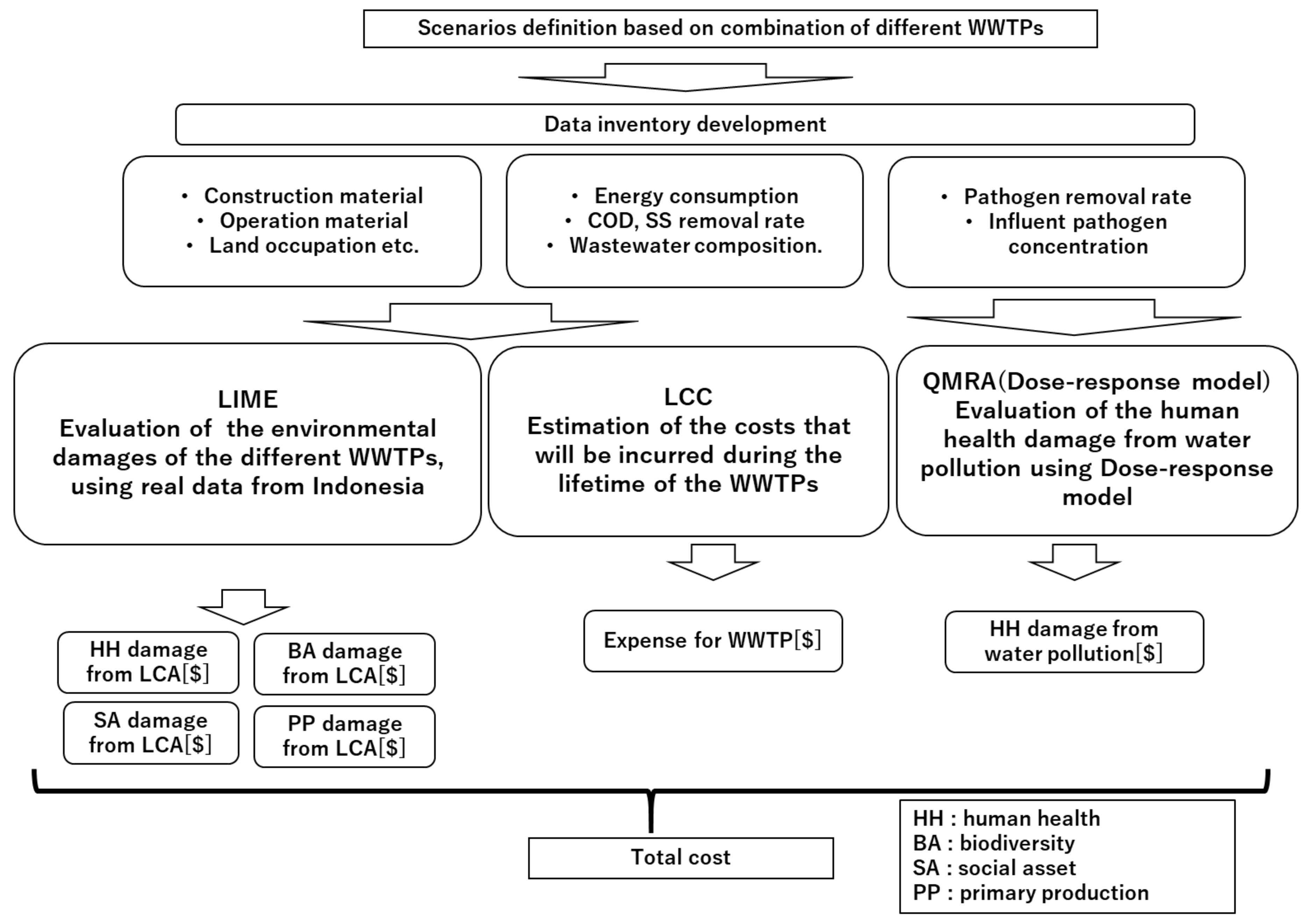
2. Model Development

Figure 1 shows a conceptual modeling framework that is proposed in this study. The modeling framework includes three main parts: (1) the LIME sub-model, which estimates environmental damages of the different WWTPs, using real data from Indonesia (2) the LCC-sub model, which estimates the life cycle cost of the different WWTPs, using cost data inventory; and (3) the QMRA model, which estimates the microbial risk of the wastewater pollution.

The LIME sub-model is used for a comprehensive endpoint assessment based on estimating damages in four endpoint groups of Human Health (HH), Social Assets (SA), Biodiversity (BD), and Primary Production (PP). HH damage indicates malnutrition and infectious diseases due to respiratory diseases caused by air pollutants such as NOx, SO₂ and photochemical ozone. SA damage includes the loss of crops and the use of minerals, and energy resources. BD damage quantifies species that are extinct due to climate change and environmental issues. PP damage is due to ecological changes that impede forest growth. Each of the endpoint domains includes different sub-categories shown in

Table 2. Definition of the sub-categories in each endpoint domain in LIME sub-model.

HH 1	BD 2	SA 3	PP 4
- Climate change - O3 - PM2.5 - Water Source	- Forest resource - Climate change - Fossil resource - Mineral resource - Land use	- Fossil resource - Mineral resource	- Forest resource - Fossil resource - Land use - Mineral resource

¹ Human Health; ² Biodiversity; ³ Social Assets; ⁴ Primary Production.

.

2.1. Weighting Method and Damage Assessment

The weighting method used in the LIME model is based on the conjoint analysis through conducting a comprehensive statistical survey in all G20 countries (including Indonesia) by different respondents. The conjoint analysis helps determine how the respondents will value different scenarios (i.e., traditional WWTP, advanced WWTP, etc.) and what combination of those scenarios is most influential in decision making, as shown in Figure 2.

Conjoint analysis is a survey-based statistical technique used in market research that helps determine how people value different attributes (feature, function, benefits) that make up an individual product or service. Based on this analysis, an individual’s overall stated preferences are decomposed into separate and compatible utility values corresponding to each attribute, typically using regression-based linear methods. Therefore a conjoint analysis extends multiple linear regression analysis to identify the weighted combination of variables to predict an outcome. The scales can be for likelihood to recommend, overall interest, or a number of other attitudes. The correlation between the damage factors can be expressed using the following linear regression model [9]:

$$V_{ij}={\beta }_1{x}_{1i}+{\beta }_2{x}_{2i}+{\beta }_3{x}_{3i}+{\beta }_4{x}_{4i}+{\beta }_{Tax}{x}_{Pi}$$

(1)

$V_{ij}$ refers to the amount of utility that the respondent (j) can receive from selecting the scenario (i). Here, the utility indicates total satisfaction from avoiding damages, which can be expressed in terms of respondents’ revealed preference. $x_{ni}$ (n: 1,2,3,4) represents the four damage factors of HH, SA, BD, and PP, respectively. ${\beta }_n$ (n: 1,2,3,4) refers to the degree of change in utility due to change in each damage factor. ${\beta }_{Tax}$ shows the degree of change in utility due to payment of one extra unit of the environmental tax ($x_{Pi}$) for avoiding different damages.

The higher the utility of a scenario to a respondent, the greater the probability that he or she will choose that scenario. Considering the logit choice rule, the probability that a respondent (j) will choose the scenario “i” among “k” possible scenarios can be expressed as follows [10]:

$$P_{ij}=\frac{exp\left(V_i\right)}{{{\displaystyle \sum }}_{k}exp\left(V_k\right)}$$

(2)

The maximum likelihood (LL) estimation is used in the conjoint analysis to estimate the parameters of a probability distribution by maximizing a likelihood function so that under the assumed statistical model, the observed data are most probable. In LIME, the likelihood function is used for estimation of the utility vectors, considering the following assumptions: (i) the vectors beta are independent random realizations from a multivariate normal distribution; (ii) the standard deviations errors are independent draws from an inverse-gamma distribution; (iii) the utility vectors among the respondents are correlated. The LL estimation method, which is used to estimate the optimal values of β can be expressed as follows [26]:

$$\mathrm{Max}\mathrm{LL}={\displaystyle \sum }_i{\displaystyle \sum }_{j}ln{P}_{ij}$$

(3)

Assuming the respondents will choose the best combination of scenarios that provides the highest utility, the estimated values of β for each type of damage, based on data collected from 200 respondents in Indonesia, are reported in

Table 3. Values of $\beta$ estimated by the LIME model [9].

$${\mathit{\beta }}_1$$	$${\mathit{\beta }}_2$$	$${\mathit{\beta }}_3$$	$${\mathit{\beta }}_4$$	$${\mathit{\beta }}_{\mathit{T}\mathit{a}\mathit{x}}{\beta }_{Tax}$$
−0.63	−0.016	−0.0069	−0.0072	−0.0023

.

According to the results, one lost day of healthy life will result in a 0.63 reduction in respondents’ utility. The marginal willingness to pay (MWTP) an extra unit of the environmental tax for avoiding different damages, can be calculated as follows [10]:

$$MWT{P}_n=\frac{{\beta }_n}{{\beta }_{Tax}}$$

(4)

The concept of MWTP was used to convert the unit of all damage factors into the monetary unit.

The HH damage due to climate change and air pollution is estimated by the following equation [9]:

$$HH=DF{a}_{HH}\times GW{P}_{}$$

(5)

$$DF{a}_{HH}=∆TEMP\times R{R}_{}\times IN{C}_{}\times CA{P}_{}\times H{D}_{}$$

(6)

where:

• HH: Total damage due to climate change [DALYs (Disability-Adjusted Life Years)]
• DFα_HH: Damage from climate change per 1 kg CO₂ emissions [DALYs/kgCO₂]
• GWP: Global Warming Potential [kgCO₂]
• ∆TEMP: Increase in temperature due to 1 [kg] of additional CO₂ emissions [°C/kgCO₂]
• RR: Rate of increase in relative risk per 1 [°C] increase in temperature [(%)/°C]
• INC: Base mortality rate [%]
• CAP: Population [people]
• HD: DALY for the death of one person [DALYs/people]

The SA damage due to loss of resources “s” (i.e., fossil fuels) can be expressed as the amount of money needed to invest a portion of the revenue generated by extracting a resource from other assets to generate similar revenue after that resource is depleted. It can be formulated as follows [10]:

$$SA=\frac{R_s{\left(\frac{1}{1+r}\right)}^{\frac{R{S}_s}{P_s}}}{P_s}\times M_s$$

(7)

• SA: Social Assets damage [$]
• R_s: Income from the extraction of resource “s” per year [$/year]
• P_s: Production of resource “s” per year [kg]
• V_s: Unit price of fossil resource “s” [$/kg]
• RS_s: Total amount of resource “s” that can be extracted [kg]
• M_s: Consumption of resource “s” [kg]
• r: Discount rate [%]

BD is estimated based on the expected increase in the number of extinct species due to the rise in temperature [10]:

$$BD=D{F}_{BD}\times GW{P}_{}$$

(8)

$$D{F}_{BD}=∆TEMP\times A_c\times L_c\times D{F}_{land,c}$$

(9)

• BD: Biodiversity Damage due to climate change [EINES (Expected Increase in Number of Extinct Species)]
• DF_BD: Expected number of extinct species form 1 [kg] CO₂ emissions [EINES/kgCO₂]
• ∆TEMP: Increase in temperature due to 1 [kg] of additional CO₂ emissions [°C/kgCO₂]
• A_c: Land area [m²]
• L_c: Growing area degradation per increase in temperature [%/°C]
• DF_land,c: Increase in the number of extinct species per 1 [m²] growing area degradation [EINES/m²]

The PP damage decreases vegetation production due to vegetation removal and changes in the vegetation’s growing environment. In the LIME, the damage is assessed using the amount of net primary production (NPP) lost per land-use area. Net primary production represents the total amount of organic matter produced by a plant in a year using solar energy, water and carbon dioxide for photosynthesis, minus the amount of organic matter lost through the plant’s respiration. The details of the calculation are given in [10].

2.2. Quantitative Microbial Risk Assessment (QMRA)

It is noted that, the LIME can only evaluate the human health damage caused by air pollution. Therefore, in order to be able to assess the health damage of wastewater pollution, a separate The QMRA model was developed based on the dose-response method and linked to the LIME. The main pathogens which were considered in the QMRA, include: (1) Escherichia coli O157:H7; (2) Salmonella spp.; (3) Campylobacter from bacteria, rotavirus, adenovirus, and norovirus from viruses, and (4) Cryptosporidium parvum and Giardia spp. from protozoa. All the selected pathogens cause gastrointestinal (GI) illness [27].

The pathogen does can be estimated, using the following formula:

$$D=C_M{V}_{ex}(1-\frac{{\eta }_{par}}{100})$$

(10)

where:

• D: pathogen dose [MPN]
• C_M: microbial concentration of the influent water [MPN/mL]
• V_ex: Quantity of the influent water [mL]
• η_ραr: removal rates of alternative technologies for various pathogens [%]
• MPN: most probable number of infectious units

The probability of infection due to microorganisms is estimated, using the following dose-response model [26]:

(a)

Beta–Poisson dose-response model:

$$P_{inf}\left(D\right)=1-{\left[1+\left(\frac{D}{N_{50}}\right)\left(2^{\frac{1}{\rho }}-1\right)\right]}^{-\rho }$$

(11)

where:

• P(D): Probability or risk of pathogen dose (D) [-]
• N₅₀: the amount of pathogen dose (D) which can infect 50% of the exposed society [MPN]
• ρ: Pathogen infectivity [-]

The Beta–Poisson model is based on the following assumptions:

-

Non-constant survival and infection probabilities.

-

Survival probabilities are given by the beta distribution.

The parameters are $\rho$ and N50. N50 is the dose at which 50% of the population is expected to be affected. Both the $\rho$ and the beta parameters are derived from the use of the beta distribution to model non-constant pathogen survival probabilities. The slope of the Beta–Poisson dose-response curve is more shallow than the exponential. The exponential model is the same as the Beta–Poisson model when alpha approaches infinity:

(b)

Exponential dose-response model

$$P_{inf}\left(D\right)=1-exp\left(-rD\right)$$

(12)

r: Model coefficient [-]

(c)

Annual risk of infection

$$P_{inf\left(A\right)}\left(D\right)=1-{\left[1-P_{inf}\left(D\right)\right]}^n$$

(13)

$P_{inf\left(A\right)}\left(D\right)$ refers to the estimated annual probability or risk of infection from “n” exposures per year due to a single pathogen dose “D”.

The health risk was expressed in disease burden, i.e., DALY per person per year as follows [26]:

$$DAL{Y}_{per person}=P_{\inf \left(A\right)}\left(D\right)\times P_{ill}\times DBPC\times f_s$$

(14)

where, $DBPC$ is the disease burden per case [DALY/year]; $f_s$ is the susceptibility fraction [-] and $P_{ill}$ is the risk of disease given infection or morbidity [-], respectively.

2.3. Life-Cycle Cost Analysis

The total cost of the system consists of construction cost, land cost, and operation cost, which can be calculated as follows:

$$Total cost=Construction cost+Land cost+ {\displaystyle \sum _{n=1}^{20}}\left\{Operation cost\times {\left(1+r\right)}^n\right\}$$

(15)

r is the discount rate, and n refers to the number of years. Operation cost consists of material, labor, maintenance, and energy costs.

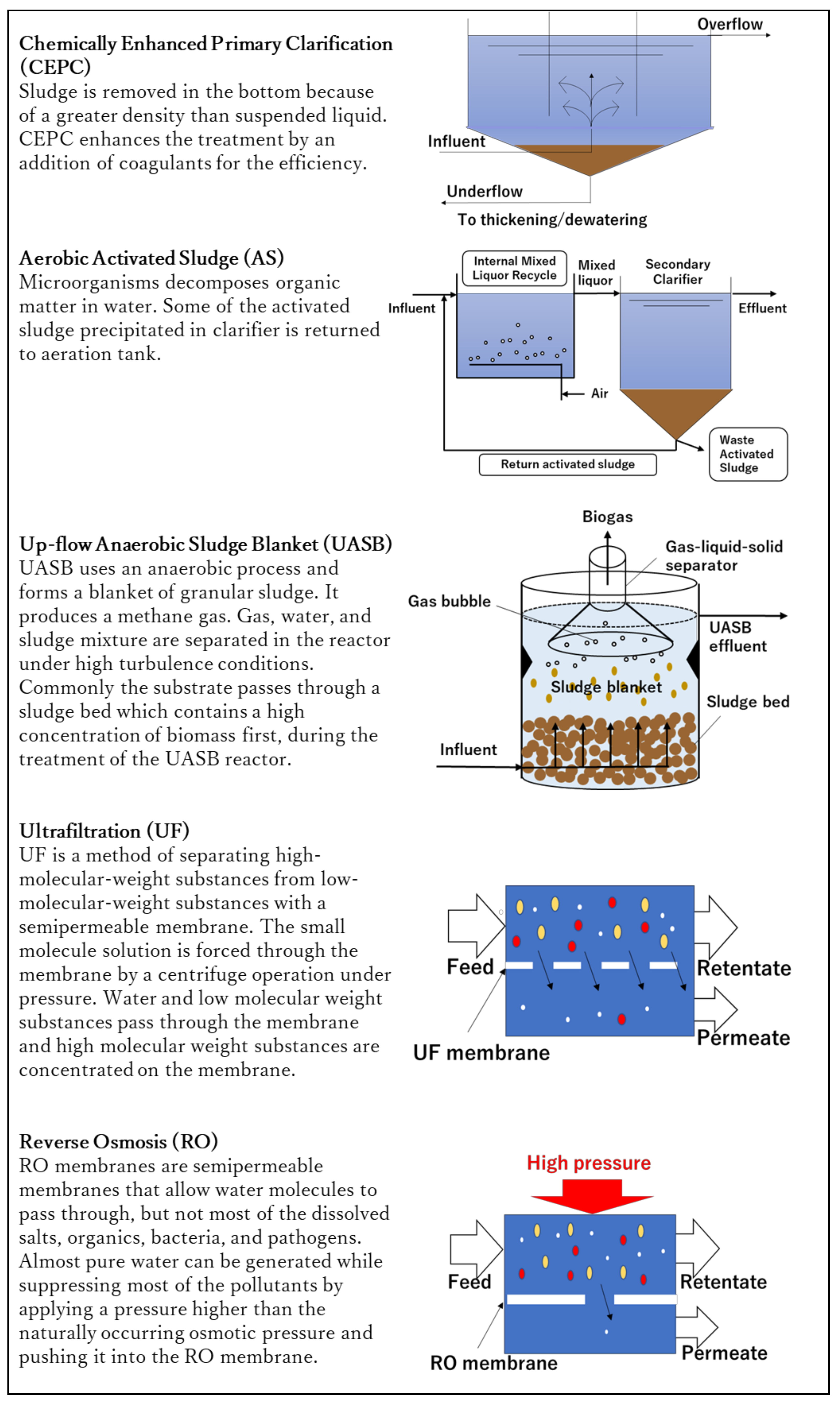
3. Case Study and Scenario Definition

Table 4. Active fish-processing factories in Indonesia [28].

Sumatera	13,947
Java	26,840
Bali	5231
Kalimantan	8880
Sulawesi	5137
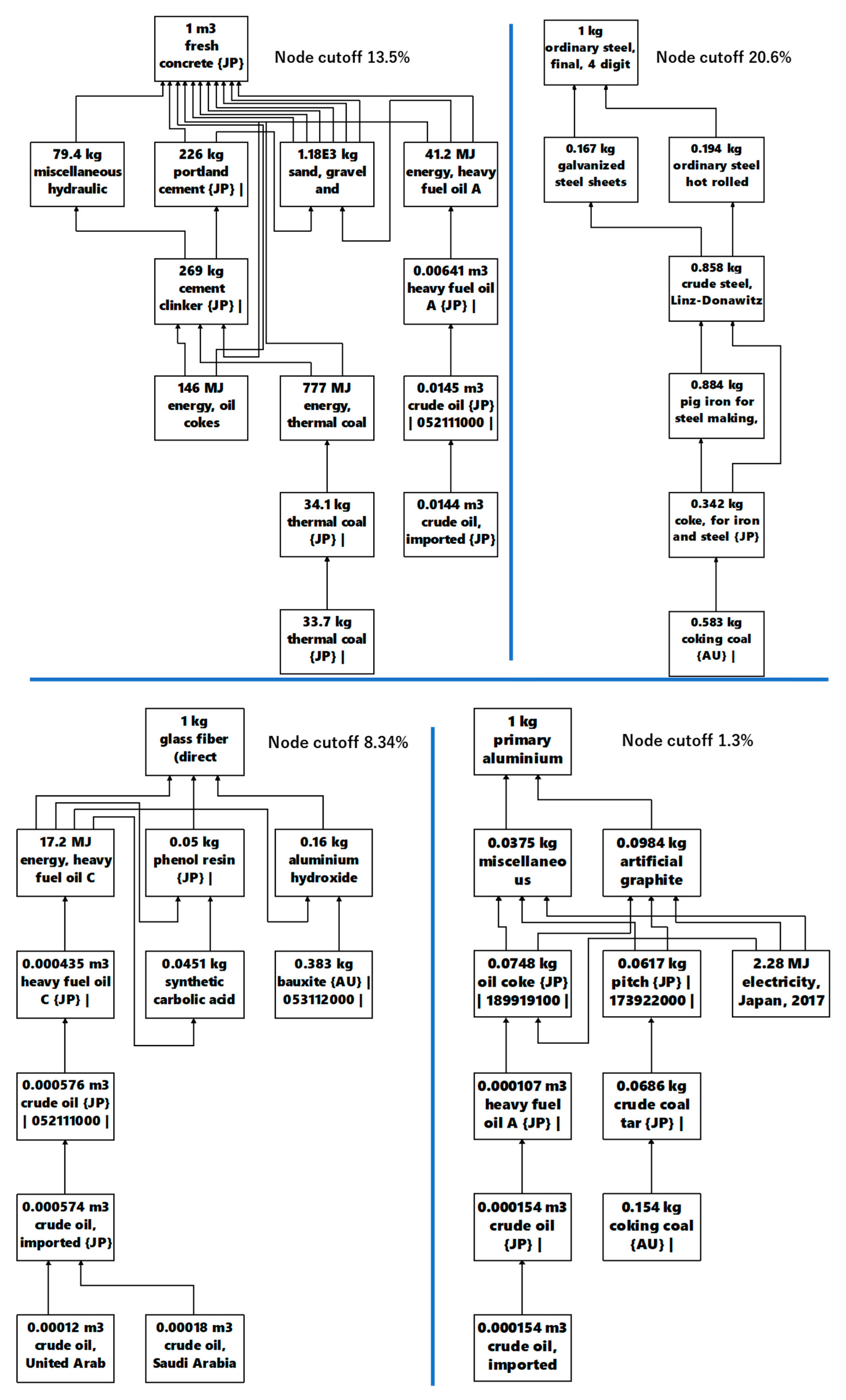
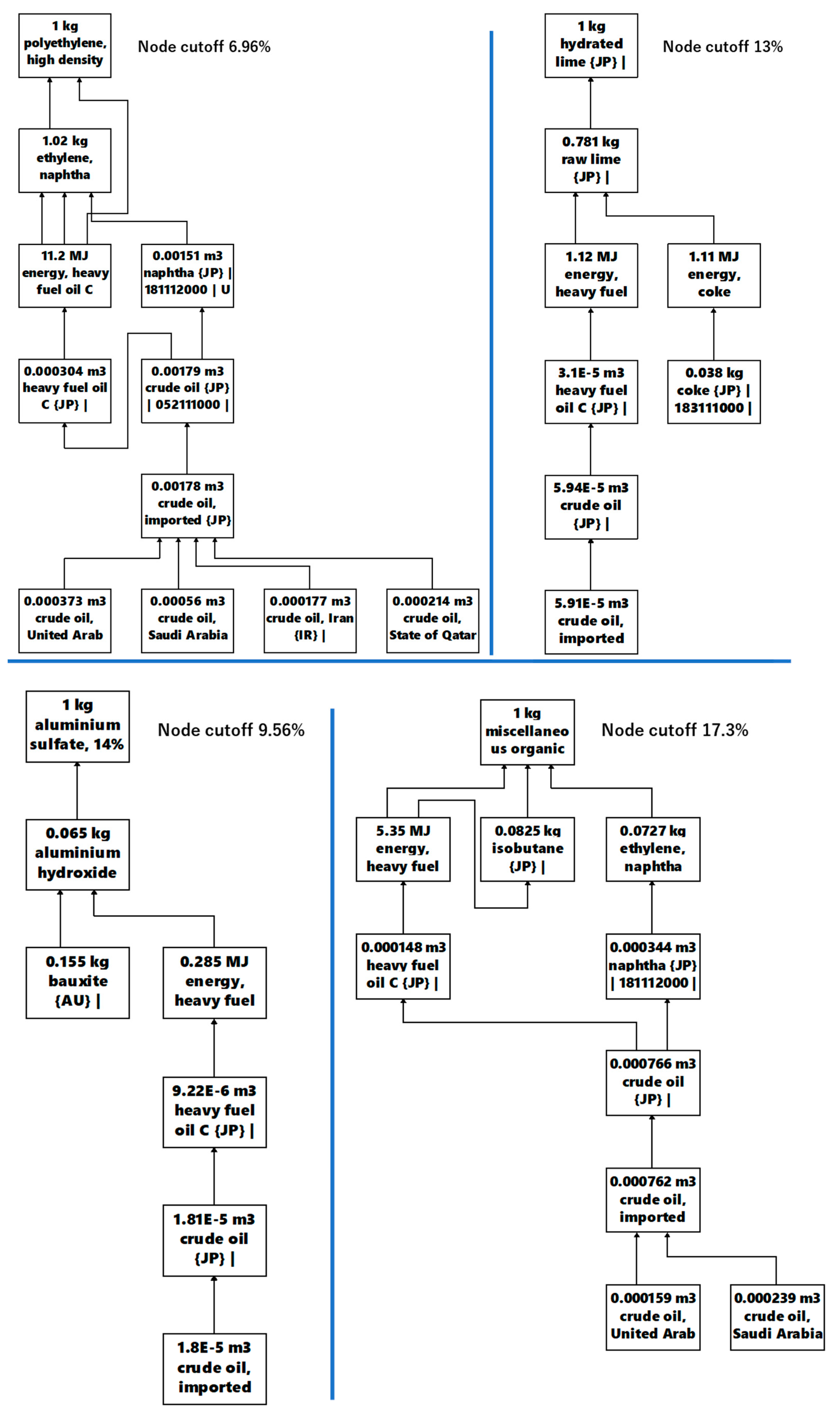
Maluku-Papua	1767

shows the number of active fish processing factories located in the different regions in Indonesia. The Java region was considered as the area of study in this research, since the major largest fish processing factories with an average influent wastewater capacity of 100 m³/d are located in this area.

Table 5. Chemical characteristics of influent wastewater in a fish-processing factory in Indonesia.

	BOD 1 [mg/L]	COD 2 [mg/L]	TSS 3 [mg/L]	SS 4 [mg/L]
Influent	1400 [28]	2900 [28]	1900 [29]	4000 [30]

¹ Biochemical Oxygen Demand; ² Chemical Oxygen Demand; ³ Total suspended solids; ⁴ Settleable Solids.

represents the chemical composition of influent wastewater used in fish-processing factories in this region.

Five main WWTPs which are considered in this study include: (1) CEPC; (2) AS; (3) UASB; (4) UF, and (5) RO. A brief description of these WWPTs is given in Figure 3. The values of the removal efficiency of the selected WWTPs are reported in

Table 6. Removal efficiency of the selected WWTPs in this study [22].

	Removal Efficiency (%)
	COD	BOD	TSS	SS
CEPC 1	54	58	86	88
AS 2	62	52	37	37
UASB 3	68	68	0	0
UF 4	77	75	96	96
RO 5	89	91	100	100

¹ Chemical-Enhanced Primary Clarification; ² Aerobic-activated Sludge; ³ Up-flow Anaerobic Sludge Blanket; ⁴ Ultrafiltration; ⁵ Reverse Osmosis.

.

In this study, nine different scenarios were considered based on possible combinations of the WWTPs, which can pass Indonesia’s standard water pollution levels. The maximum concentration of biochemical oxygen demand (BOD), chemical oxygen demand (COD), and total suspended solids (TSS) in the discharged wastewater is allowed to be 75 (mg/L), 150 (mg/L), and 100 (mg/L), respectively [16]. The scenario definition and water pollution levels in effluent water in each scenario are given in

Table 7. Scenario definition in this study.

Scenario No.	Primary Treatment	Secondary Treatment	Tertiary Treatment
1	CEPC	AS	UF
2	CEPC	UASB	UF
3	CEPC	AS + UASB	UF
4	CEPC	AS	RO
5	CEPC	UASB	RO
6	CEPC	AS + UASB	RO
7	CEPC	AS	UF + RO
8	CEPC	UASB	UF + RO
9	CEPC	AS + UASB	UF + RO

and

Table 8. Water pollution levels in effluent water of the proposed scenarios.

Scenario No.	BOD Concentration [mg/L]	COD Concentration [mg/L]	SS Concentration [mg/L]
1	56.3	146	18.8
2	47.4	97.4	29.8
3	18.0	46.8	18.8
4	26.9	52.6	0.00
5	22.7	35.1	0.00
6	8.61	16.8	0.00
7	6.19	13.2	0.00
8	5.21	8.77	0.00
9	1.98	4.21	0.00

.

4. Data Inventory

The LCA data inventory denotes the appropriate inputs and outputs from each WWTP. Inventory flows in this study include inputs of water, material, energy, land, and energy carriers and outputs of air and water pollutions.

Table 9. Basic components used in the selected WWTPs in this study.

Component	CEPC	AS	UASB	UF	RO
Construction [$\mathrm{kg}/{\mathrm{m}}^3$] 1
Frech concrete	0.0360 [32,33]	0.0780 [33]	0.0120 [33]	0.00300 [34]	0.00328 [32]
Ordinary steel	0.00128 [30,31]	0.00276 [33]	0.000425 [33]	0.000760 [34]	0.000760 [34]
Glass fiber (direct roving)	0.0000294 [33]	0.0000637 [33]	0.00000998 [33]	0.000150 [34]	0.000150 [34]
Aluminum	0.0000131 [33]	0.0000283 [33]	0.00000435 [33]	0	0
Polyethylene, high density (HDPE)	0	0.0000793 [33]	0.0000122 [33]	0	0
Operation (Chemicals) [mg/L] 2
Hydrated lime	400 [35]	0	0	0	0
Aluminium sulfate, 14% solution	10 [35]	0	0	0	0
Anionic surface-activate agents (Anionic polymer)	6 [35]	0	0	0	0
Sodium hydroxide, 97%	0	0	0	4.20 [34]	4.20 [34]
Nitric acid, 98%	0	0	0	1.85 [36]	0
Plastic products which are not elsewhere classified (Filters for the prefilters)	0	0	0	0.260 [34]	0.260 [34]
Ultrafiltration Spiral wound modules	0	0	0	0.510 [34]	0.510 [34]
Land occupation [${\mathrm{m}}^2/\mathrm{PE}$] 3				Land occupation [${\mathrm{m}}^2/{\mathrm{m}}^3/\mathrm{d}$]
Resources, building site, land use, land occupation	0.05 [37]	0.185 [37]	0.065 [37]	0.083 [38]	0.25 [38]
Electricity consumption [$\mathrm{kWh}/{\mathrm{m}}^3$] 1
Electricity, Indonesia	0.38 [22]	1.03 [22]	0.37 [22]	0.94 [22]	1.90 [22]

¹ Cubic meter of treated water; ² Liter of treated water; ³ Population equivalent.

shows the basic components used in the construction, operation, and land occupation of the selected WWTPs.

Land occupation data for CEPC, AS, and UASB are given per population equivalent (PE). PE represents the ratio of the daily load of the discharged wastewater from the industrial factories to the load of sewage produced by an inhabitant in the household area [39,40]:

$$Population equivalent \left[PE\right]=\frac{BOD load from industry \left[\mathrm{kg}/\mathrm{d}\right]}{per capita BOD load \left[\mathrm{kg}/\left(\mathrm{inhab}\times \mathrm{day}\right)\right]}$$

(16)

The value of the BOD per capita is estimated at $54 \left[\mathrm{g}/\left(\mathrm{inhab}\times \mathrm{day}\right)\right]$.

The LIME comprehensive database was used for inventory regarding the different construction and operation and electricity generation processes in this study. The overall structure of the data inventory flows used in LIME is shown in Figure 4.

The unit costs of raw material, electricity, land, and energy are reported in

Table 10. Unit costs of raw material, electricity, land, and energy used in this study.

Items	Value	Unit	Reference
Electricity	1051	$\mathrm{Rp}/\mathrm{kWh}$	[41]
Land	17.93	$\text{\$}/{\mathrm{ft}}^2$	[42]
Labor	183	$\text{\$}/\mathrm{people}/\mathrm{month}$	[43]
Steel	504	$\text{\$}/\mathrm{ton}$	[44]
Fiberglass	625	$\text{\$}/\mathrm{ton}$	[45]
Aluminum	1777	$\text{\$}/\mathrm{ton}$	[46]
Lime	17	$\mathrm{Rs}/\mathrm{kg}$	[47]
Anionic polymer	1.25	$\text{\$}/\mathrm{pound}$	[48]
Concrete	300	$\text{\$}/{\mathrm{m}}^3$	[49]
HDPE	54.81	$\text{¢}/\mathrm{pound}$	[50]
Alum	120	$\mathrm{Rs}/\mathrm{kg}$	[51]
Membrane cleaning agent (NaOH)	375	$\text{\$}/\mathrm{ton}$	[52]
Nitric Acid	262.5	$\text{\$}/\mathrm{ton}$	[53]
Filters	889	$\mathrm{JPY}/\mathrm{p}\left(215\mathrm{kg}\right)$	[54]
UF spiral-wound modules	800	$\text{\$}/\mathrm{p}\left(26\mathrm{kg}\right)$	[55]

.

The average labor load for the selected WWPTs is given in

Table 11. Average labor load for the selected WWTPs.

WWTP	Labor/Year
CEPC, AS and USAB	13
UF	17 [38]
RO	12 [38]

.

The amount of solid waste generated from the WWTPs was estimated based on the amount of removed settleable solids from the influent wastewater. Water pollution was calculated based on COD and TSS concentration in the discharged water from the WWTPs. It is assumed that drinking discharged water from the WTTPs will cause gastrointestinal (GI) illness. The quantity of the influent water ($V_{ex}$) and frequency per year (n) are reported in

Table 12. Quantity of the influent water and its frequency per person.

Exposure Source	${\mathit{V}}_{\mathit{e}\mathit{x}}\left[\mathbf{mL}\right]$	Frequency per Year n [th/year]
Drinking	2800 [56]	365

.

The pathogen removal rates of the selected WPPTs and input parameters used in the QMRA are given in

Table 13. The log removal (${\eta }_{Log}$) of the selected WTTPs for various pathogens ¹.

	E. coli [-]	Campylobacter [-]	Salmonella spp. [-]	Adenoviruses [-]	Noroviruses [-]	Rotavirus [-]	Cryptosporidium [-]	Giardia spp. [-]	Reference
CEPC	1.06	0.955	0.955	2.6	2.6	2.6	0.14	0.62	[57]
AS	1.5	1.5	1.5	1.25	1.25	1.25	0.75	0.75	[58]
UASB	1.1	1.2	1	0.7	0.2	0	0.3	0.3	[59]
UF	5	5	4.5	4.5	4.5	6.2	6.35		[60]
RO	5.5	5.5	5.5	4.85	4.85	4.85	8	8	[61]

¹${\eta }_{par}=100\times \left(1-{10}^{-{\eta }_{Log}}\right)$.

,

Table 14. The microbial concentration of influent water.

Microorganisms	$\mathbf{Concentration}[\mathit{M}\mathit{P}\mathit{N}/100\mathbf{mL}]$	Reference
E. coli	31,622,777	[58]
Campylobacter	3162	[59]
Salmonella spp.	10,000	[58]
Adenoviruses	316	[58]
Noroviruses	316	[58]
Rotavirus	3162	[58]
Cryptosporidium	100	[59]
Giardia spp.	3162	[59]

and

Table 15. Input parameters used in the QMRA.

Pathogens	Beta-Poisson		Exponential	Reference
	$\mathit{\rho }$ [-]	N50 [-]	r [-]
E. coli	0.2019	1120	–	[58]
Salmonella spp.	0.3126	23,600	–	[62]
Adenovirus	–	–	0.4172	[63]
Norovirus	–	–	0.722	[64]
Campylobacter	0.145	896	–	[65]
Rotavirus	0.27	5.6	–	[66]
Cryptosporidium parvum	–	–	0.004	[67]
Giardia spp.	–	–	0.0199	[68]

.

The values of morbidity, disease burden per case, and susceptibility fraction are shown in

Table 16. Morbidity, disease burden per case, and susceptible fraction.

Pathogens	$\mathbf{Morbidity}{\mathit{P}}_{\mathit{i}\mathit{l}\mathit{l}|\mathit{i}\mathit{n}\mathit{f}}[-]$	Maximum Disease Burden [DALY 1/year]	Susceptibility Fraction ${\mathit{f}}_{\mathit{s}}[-]$	Reference
E. coli	0.4	0.055	0.9	[69]
Campylobacter	0.35	0.00335	0.9	[70]
Salmonella spp.	0.2	0.0446	0.9	[71]
Adenovirus	0.5	0.0534	0.9	[71]
Norovirus	0.55	0.0006	0.9	[70]
Rotavirus	0.67	0.0084	0.06	[70]
Cryptosporidium	0.45	0.00195	0.9	[69]
Giardia spp.	0.45	0.00225	0.9	[69]

¹ Disability-Adjusted Life Year.

.

5. Results and Discussion

The SimaPro 7.1.8 software was used to carry out the LCA in this study. The results of the assessment in four endpoint categories of HH, SA, BD, and PP are reported in

Table 17. Endpoint assessment results in the selected scenarios, including total damage.

Scenario	HH1 1		HH2 2		PP		SA	BD		Total Damage
	DALYs	1000$	DALYs	1000$	Ton	1000$	1000$	$({10}^{-6} \mathbf{EINES})$	1000$	1000$
1	$1.19$	$29.9$	$28.1$	$702$	$56.3$	$3.10$	$92.6$	$2.75$	$14.6$	$842$
2	$0.896$	$22.4$	$28.7$	$717$	$43.8$	$2.41$	$69.5$	$2.11$	$11.2$	$822$
3	$1.36$	$34.0$	$27.2$	$680$	$62.8$	$3.46$	$105$	$3.10$	$16.4$	$839$
4	$1.62$	$40.6$	$27.9$	$697$	$72.6$	$3.99$	$126$	$3.66$	$19.4$	$887$
5	$1.32$	$33.1$	$28.4$	$709$	$60.1$	$3.31$	$103$	$3.02$	$16.0$	$864$
6	$1.79$	$44.7$	$19.4$	$486$	$79.1$	$4.35$	$138$	$4.01$	$21.3$	$694$
7	$2.05$	$51.2$	$0$	$0$	$89.2$	$4.91$	$160$	$4.58$	$24.3$	$240$
8	$1.75$	$43.8$	$0$	$0$	$76.7$	$4.22$	$137$	$3.94$	$20.9$	$206$
9	$2.22$	$55.4$	$0$	$0$	$95.7$	$5.27$	$172$	$4.93$	$26.1$	$259$

¹ Human health damage caused by air pollution calculated by the LIME; ² Human health damage due to microbial diseases caused by wastewater pollution calculated by the QMRA model.

.

As can be observed from the results, there are fewer adverse impacts associated with the endpoint categories of HH1, SA, and BD in scenarios 1–6 than others. On the other hand, the estimated damage due to microbial diseases (HH2) is almost zero in scenario 7–9. Although the combined use of UF and RO technologies in secondary and secondary treatment processes has led to an increase in total electricity consumption, it has reduced the health damage caused by microbial diseases, which significantly reduces the overall environmental damage in Scenarios 7–9. Figure 5 represents how the combination of the UF and RO technologies in the tertiary treatment has led to a significant improvement in pathogen removal efficiency in these scenarios.

Among scenarios 7–9, scenario 8 performs better in reducing the total damages. In this scenario, UASB technology is employed in the secondary treatment process, which uses less electricity, due to utilizing biogas to supply the required electricity for wastewater treatment. Conversely, scenario 4 is the worst scenario with the most adverse impacts associated with all endpoint categories. This scenario deploys AS and RO technologies for the secondary and tertiary treatment processes separately, resulting in a large amount of electricity consumption in the whole treatment process. Besides, due to the low pathogen removal rate of the treatment technology, the rate of DALYs caused by E. coli has increased in this scenario (See

Table 18. Estimation of the DALYs caused by the E. coli in the selected scenario.

Scenario No.	${\mathit{P}}_{\mathit{i}\mathit{n}\mathit{f}}\left(\mathit{d}\right)$$\left[-\right]$	${\mathit{P}}_{\mathit{i}\mathit{n}\mathit{f}\left(\mathit{A}\right)}\left(\mathit{d}\right)$$\left[-\right]$	$\mathit{D}\mathit{A}\mathit{L}{\mathit{Y}}_{\mathit{p}\mathit{e}\mathit{r} \mathit{y}\mathit{e}\mathit{a}\mathit{r}} *$
1	$9.65\times {10}^{-2}$	$1$	$1.39$
2	$1.78\times {10}^{-2}$	$1$	$1.39$
3	$1.02\times {10}^{-2}$	$0.976$	$1.36$
4	$3.72\times {10}^{-2}$	$1$	$1.39$
5	$8.09\times {10}^{-2}$	$1$	$1.39$
6	$3.28\times {10}^{-3}$	$0.698$	$9.70\times {10}^{-1}$
7	$4.16\times {10}^{-7}$	$1.52\times {10}^{-4}$	$2.11\times {10}^{-4}$
8	$1.05\times {10}^{-6}$	$3.82\times {10}^{-4}$	$5.31\times {10}^{-4}$
9	$3.26\times {10}^{-8}$	$1.19\times {10}^{-5}$	$1.65\times {10}^{-5}$

* Assuming a WPPTs with 100 m³/d influent capacity.

).

Figure 6 represents the adverse impact associated with each endpoint category in the selected scenarios.

As can be observed from this figure, the most adverse impact is associated with human health damage due to microbial diseases (HH2) in scenarios 1–6, mainly due to the low-efficiency water treatment process in these scenarios. Electricity consumption-related air pollution such as PM_2.5 made a significant adverse impact in the HH1 category for all scenarios, which is due to a direct relationship between PM_2.5 inhalation and the development of respiratory and cardiovascular diseases. Electricity consumption also made negative impacts in the SA category for each scenario. With the consumption of fossil resources, resource reserves are depleted as a social capital, which leads to increased resource royalties and costs related to resource extraction. Energy-related climate change negatively affects the climate-friendly areas needed for living organisms’ growth and causes significant biodiversity damage. Figure 7 represents the effect of electricity consumption on total environmental damage in each scenario.

The LCC result is reported in

Table 19. Results of the LCC in the selected scenario.

Scenario No.	Construction Cost 10,000 [$]	Land Cost 10,000 [$]	Annual Operation 10,000 [$/Y]	LCC * 10,000 [$]
1	$8.14$	$7.14$	$1.22$	$48.1$
2	$3.70$	$4.29$	$1.05$	$36.2$
3	$9.09$	$7.73$	$1.34$	$52.7$
4	$8.28$	$7.48$	$1.47$	$55.1$
5	$3.72$	$4.63$	$1.29$	$43.1$
6	$9.11$	$8.06$	$1.58$	$59.6$
7	$8.68$	$7.64$	$1.83$	$65.6$
8	$4.12$	$4.79$	$1.66$	$53.5$
9	$9.51$	$8.23$	$1.95$	$70.0$

* Discount rate was assumed at 3%.

, which includes construction, land, and annual operation costs. The major cost item in all scenarios is construction cost, which is followed by the land cost. The LCC in scenario 9 is the highest among all the scenarios, which can be attributed to the increased capital investment for the combination of advanced technologies such as AS + UASB in the secondary treatment and UF + RO in the tertiary treatment processes. Furthermore, the land use in this scenario is very high compared to the standard requirement for a regular WWTP.

Figure 8 compares the environmental damages cost with the total life-cycle cost in the selected scenario. The environmental damage cost is higher in scenario 1–6, mainly due to lower pathogen removal efficiency. Therefore, the most significant environmental damage cost is attributed to the human health damage caused by wastewater pollution (HH2). The opposite was observed in scenarios 7–9. The utilization of UASB technology in the secondary treatment process and the addition of the UF to RO in the tertiary treatment process have reduced the cost of environmental damage.

6. Conclusions

Nine different wastewater treatment scenarios in Indonesia’s fish-processing industry were environmentally evaluated by the LCA technique used in the LIME-based method. The scenarios were selected, considering the combination of different conventional and advanced technologies in both secondary and tertiary treatment processes. The LCA was carried out to assess the adverse impact on the environment in four endpoint categories of Human Health (HH), Social Assets (SA), Biodiversity (BD), and Primary Production (PP). The LCA results revealed that air pollution and gaseous emissions from electricity consumption have the most significant environmental impacts in all scenarios and all categories. The adverse impacts of water pollution are more important than air pollution, especially in scenarios in which conventional technologies with lower bacterial removal efficiency are used in the tertiary treatment process. The up-flow anaerobic sludge blanket (UASB) system showed lower impacts on the environment compared to the traditional systems such as activated sludge (AS), due to the replacement of the purchased electricity with the electricity generated from the produced biogas. Merging ultrafiltration (UF) and reverse osmosis (RO) in the tertiary treatment process were very beneficial for all impact categories due to improved effluent water quality. The cost estimation of the selected scenarios revealed that the environmental benefits attained from the 7th, 8th, and 9th scenarios could lower the treatment system’s cost over a long period.

References

1. Gómez-Sanabria, A.; Zusman, E.; Höglund-Isaksson, L.; Klimont, Z.; Lee, S.; Akahoshi, K.; Farzaneh, H.; Chairunnisa. Sustainable wastewater management in Indonesia’s fish processing industry: Bringing governance into scenario analysis. J. Environ. Manag. 2020, 275, 111241. [Google Scholar]
2. Farzaneh, H. Devising a Clean Energy Strategy for Asian Cities; Springer: New York, NY, USA, 2018. [Google Scholar]
3. Muga, H.E.; Mihelcic, J.R. Sustainability of wastewater treatment technologies. J. Environ. Manag. 2008, 88, 437–447. [Google Scholar] [CrossRef] [PubMed]
4. Hellweg, S.; Mila, I.; Canals, L. Emerging approaches, challenges and opportunities in life cycle assessment. Science 2014, 344, 1109–1113. [Google Scholar] [CrossRef] [PubMed]
5. Awad, H.; Gar Alalm, M.; El-Etriby, H.K. Environmental and cost life cycle assessment of different alternatives for improvement of wastewater treatment plants in developing countries. Sci. Total Environ. 2019, 660, 57–68. [Google Scholar] [CrossRef]
6. Lopes, T.A.; Queiroz, L.M.; Torres, E.A.; Kiperstok, A. Low complexity wastewater treatment process in developing countries: A LCA approach to evaluate environmental gains. Sci. Total Environ. 2020, 720, 137593. [Google Scholar] [CrossRef]
7. Lorenzo-Toja, Y.; Vázquez-Rowe, I.; Chenel, S.; Marín-Navarro, D.; Moreira, M.T.; Feijoo, G. Eco-efficiency analysis of Spanish WWTPs using the LCA + DEA method. Water Res. 2015, 68, 651–666. [Google Scholar] [CrossRef]
8. Larrey-Lassalle, P.; Catel, L.; Roux, P.; Rosenbaum, R.K.; Lopez-Ferber, M.; Junqua, G.; Loiseau, E. An innovative implementation of LCA within the EIA procedure: Lessons learned from two wastewater treatment plant case studies. Environ. Impact Assess. Rev. 2017, 63, 95–106. [Google Scholar] [CrossRef]
9. Hao, X.; Wang, X.; Liu, R.; Li, S.; van Loosdrecht, M.C.M.; Jiang, H. Environmental impacts of resource recovery from wastewater treatment plants. Water Res. 2019, 160, 268–277. [Google Scholar] [CrossRef]
10. Itsubo, N.; Inaba, A. LIME3: Environmental Impact Assessment Method for Realizing Global Scale LCA; Maruzen Publishing: Tokyo, Japan, 2018. (In Japanese) [Google Scholar]
11. Bai, S.; Wang, X.; Huppes, G.; Zhao, X.; Ren, N. Using site-specific life cycle assessment methodology to evaluate Chinese wastewater treatment scenarios: A comparative study of site-generic and site-specific methods. J. Clean. Prod. 2017, 144, 1–7. [Google Scholar] [CrossRef]
12. Lu, B.; Du, X.; Huang, S. The economic and environmental implications of wastewater management policy in China: From the LCA perspective. J. Clean. Prod. 2017, 142, 3544–3557. [Google Scholar] [CrossRef]
13. Nguyen, T.K.; Ngo, H.H.; Guo, W.; Chang, S.W.; Nguyen, D.D.; Nguyen, T.V.; Nghiem, D.L. Contribution of the construction phase to environmental impacts of the wastewater treatment plant. Sci. Total Environ. 2020, 743, 140658. [Google Scholar] [CrossRef]
14. Yokoi, R.; Nakatani, J.; Motoshita, M.; Moriguchi, Y. Calculation and comparison of weighting factors based on different methods in life cycle impact assessment. J. Life Cycle Assess. Jpn. 2015, 11, 278–291. [Google Scholar] [CrossRef] [Green Version]
15. 2013 Graduation Research Topic 3. Impact Assessment of LCA. Available online: http://www.urm.t.u-tokyo.ac.jp/research/graduation2013_2.pdf (accessed on 15 July 2020). (In Japanese).
16. Barjoveanu, G.; Comandaru, I.M.; Rodriguez-Garcia, G.; Hospido, A.; Teodosiu, C. Evaluation of water services system through LCA. A case study for Iasi city, Romania. Int. J. Life Cycle Assess. 2013, 19, 449–462. [Google Scholar] [CrossRef]
17. Risch, E.; Loubet, P.; Núñez, M.; Roux, P. How environmentally significant is water consumption during wastewater treatment? Application of recent developments in LCA to WWT technologies used at 3 contrasted geographical locations. Water Res. 2014, 57, 20–30. [Google Scholar] [CrossRef]
18. Thibodeau, C.; Monette, F.; Bulle, C.; Glaus, M. Comparison of Black water source-separation and conventional sanitation systems using life cycle assessment. J. Clean. Prod. 2014, 67, 45–57. [Google Scholar] [CrossRef]
19. Lam, L.; Kurisu, K.; Hanaki, K. Comparative environmental impacts of source-separation systems for domestic wastewater management in rural China. J. Clean. Prod. 2015, 104, 185–198. [Google Scholar] [CrossRef]
20. Fuchs, V.J.; Mihelcic, J.R.; Gierke, J.S. Life cycle assessment of vertical and horizontal flow constructed wetlands for wastewater treatment considering nitrogen and carbon greenhouse gas emissions. Water Res. 2011, 45, 2073–2081. [Google Scholar] [CrossRef]
21. Buonocore, E.; Mellino, S.; De Angelis, G.; Liu, G.; Ulgiati, S. Life cycle assessment indicators of urban wastewater and sewage sludge treatment. Ecol. Indic. 2018, 94, 13–23. [Google Scholar] [CrossRef]
22. O’Connor, M.; Garnier, G.; Batchelor, W. Life cycle assessment comparison of industrial effluent management strategies. J. Clean. Prod. 2014, 79, 168–181. [Google Scholar] [CrossRef]
23. Amini, A.; Kim, Y.; Zhang, J.; Boyer, T.; Zhang, Q. Environmental and economic sustainability of ion exchange drinking water treatment for organics removal. J. Clean. Prod. 2015, 104, 413–421. [Google Scholar] [CrossRef]
24. Hong, J.; Hong, J.; Otaki, M.; Jolliet, O. Environmental and economic life cycle assessment for sewage sludge treatment processes in Japan. Waste Manag. 2009, 29, 696–703. [Google Scholar] [CrossRef] [PubMed]
25. Harder, R.; Peters, G.M.; Molander, S.; Ashbolt, N.J.; Svanström, M. Including pathogen risk in life cycle assessment: The effect of modelling choices in the context of sewage sludge management. Int. J. Life Cycle Assess. 2015, 21, 60–69. [Google Scholar] [CrossRef] [Green Version]
26. AVILEN AI Trend. Available online: https://ai-trend.jp/basic-study/estimator/likehood-score-fisher/ (accessed on 1 December 2020). (In Japanese).
27. Chhipi-Shrestha, G.; Hewage, K.; Sadiq, R. Fit-for-purpose wastewater treatment: Conceptualization to development of decision support tool (I). Sci. Total Environ. 2017, 607–608, 600–612. [Google Scholar] [CrossRef] [PubMed]
28. Nihon Suido Consultants Co., Ltd. 2017 Indonesian Fisheries Processing Industry Co-Benefit Wastewater Countermeasure Survey Commissioned Business Report; Nihon Suido Consultants Co., Ltd.: Tokyo, Japan, 2018; pp. 43, 54, 404, 417. (In Japanese) [Google Scholar]
29. Freire, C.S.; Silvestre, A.J.; Neto, C.P. Carbohydrate-derived chlorinated compounds in ECF bleaching of hardwood pulps: Formation, degradation, and contribution to AOX in a bleached Kraft pulp mill. Environ. Sci. Technol. 2003, 37, 811–814. [Google Scholar] [CrossRef] [PubMed]
30. Žarković, D.B.; Todorović, Ž.N.; Rajaković, L.V. Simple and cost-effective measures for the improvement of paper mill effluent treatment—A case study. J. Clean. Prod. 2011, 19, 764–774. [Google Scholar] [CrossRef]
31. EPA. The United States Environmental Protection Agency. Emerging Technologies for Wastewater Treatment and In-Plant Wet Weather Management. 2013. Available online: https://www.epa.gov/sites/production/files/2019-02/documents/emerging-tech-wastewater-treatment-management.pdf (accessed on 17 September 2020).
32. Doka, G. Life cycle inventory of wastewater treatment. Part IV Chapter 4. In Life Cycle Inventories of Waste Treatment Services; Ecoinvent Report No. 13; Swiss Centre for Life Cycle Inventories: Dubendorf, Switzerland, 2003. [Google Scholar]
33. Foley, J.; De Haas, D.; Hartley, K.; Lant, P. Comprehensive life cycle inventories of alternative wastewater treatment systems. Water Res. 2010, 44, 1654–1666. [Google Scholar] [CrossRef] [PubMed]
34. Bonton, A.; Bouchard, C.; Barbeau, B.; Jedrzejak, S. Comparative life cycle assessment of water treatment plants. Desalination 2012, 284, 42–54. [Google Scholar] [CrossRef]
35. Buyukkamaci, N.; Koken, E. Economic evaluation of alternative wastewater treatment plant options for pulp and paper industry. Sci. Total Environ. 2010, 408, 6070–6078. [Google Scholar] [CrossRef]
36. Pizzichini, M.; Russo, C.; Meo, C.D. Purification of pulp and paper wastewater, with membrane technology, for water reuse in a closed loop. Desalination 2005, 178, 351–359. [Google Scholar] [CrossRef]
37. Von Sperling, M. Wastewater characteristics, treatment and disposal. Water Intell. Online 2015, 6, 224–225. [Google Scholar] [CrossRef]
38. Plakas, K.V.; Georgiadis, A.A.; Karabelas, A.J. Sustainability assessment of tertiary wastewater treatment technologies: A multi-criteria analysis. Water Sci. Technol. 2015, 73, 1532–1540. [Google Scholar] [CrossRef]
39. European Environment Agency. Glossary of Terms Related to Urban Waste Water. 2020. Available online: https://www.eea.europa.eu/help/glossary/eea-glossary/population-equivalent (accessed on 17 September 2020).
40. Nsavyimana, G.; Kaboneka, S.; Bigumandondera, P.; Ngahane, E.L.; Ndikumana, T.; Vasel, J.L. Exploring a new approach of the population equivalent concept through a detailed characterization of grey and Black waters. Int. J. Adv. Sci. Res. Eng. 2020, 6, 32–49. [Google Scholar] [CrossRef]
41. International Energy Situation Survey. 2017. Available online: https://www.meti.go.jp/meti_lib/report/H29FY/000219.pdf (accessed on 17 September 2020). (In Japanese).
42. Average Land Price in Greater Jakarta Q1 2019, by Region. Available online: https://www.statista.com/statistics/1042205/indonesia-average-land-price-in-greater-jakarta/ (accessed on 17 September 2020).
43. Indonesia Monthly Earnings. Available online: https://www.ceicdata.com/en/indicator/indonesia/monthly-earnings (accessed on 17 September 2020).
44. World Steel Prices. Available online: https://worldsteelprices.com/ (accessed on 17 September 2020).
45. Made in China TM. Available online: https://tianmagroup.en.made-in-china.com/product/rjAxvRBPHmkZ/China-E-Glass-Fiberglass-Direct-Roving-for-Winding-EDR2400-T908.html (accessed on 17 September 2020).
46. Trading Economics. Available online: https://tradingeconomics.com/commodity/aluminum (accessed on 17 September 2020).
47. Lime Price Per kg. Available online: https://motormatcher.com.au/forum/lime-price-per-kg-f644a7 (accessed on 17 September 2020).
48. City of Bloomington Illinois. Available online: https://www.cityblm.org/Home/ShowDocument?id=10595 (accessed on 17 September 2020).
49. Cost of Concreting Per m3 (Cubic Metre). Available online: https://www.serviceseeking.com.au/blog/concrete-cost-per-cubic-metre/#:~:text=The%20supply%20cost%20of%20concreting,concreters%20run%20from%20%2480%2Fhr (accessed on 17 September 2020).
50. Plastics Recycling Update. Available online: https://resource-recycling.com/plastics/2020/02/12/hdpe-prices-fall-from-record-highs/#:~:text=The%20national%20average%20price%20of%20color%20HDPE%20dropped%20again%20this,at%2012.47%20cents%20per%20pound (accessed on 17 September 2020).
51. Baniyababu.com. Available online: http://baniyababu.com/product/grocery-and-staples/turti-alum-1-kg/ (accessed on 17 September 2020).
52. Nikkei Asin Review. Available online: https://asia.nikkei.com/Business/Markets/Commodities/Caustic-soda-prices-on-upward-trend-in-Asian-markets (accessed on 17 September 2020).
53. Chemical Profile: Nitric Acid. Available online: https://www.icis.com/explore/resources/news/2008/05/19/9124327/chemical-profile-nitric-acid/ (accessed on 17 September 2020).
54. Monotaro. Available online: https://www.monotaro.com/g/01240073/?t.q=%83%7C%83%8A%83v%83%8D%83s%83%8C%83%93%83t%83B%83%8B%83%5E%81%5B%20%8E%BF%97%CAspm=a2700.7724857.normalList.26.5770df268OjVeQ&s=p (accessed on 17 September 2020). (In Japanese).
55. Alibaba.com. Available online: https://www.alibaba.com/product-detail/UFf160-Polyvinylidine-fluoride-PVDF-spiral-wound_60838240576.html?spm=a2700.7724857.normalList.81.67c1c0a5Uzi1Es (accessed on 17 September 2020).
56. David, W.; Widianingsih, N.N.; Ploeger, A. Water usage pattern on different group residing in vicinity Harapan rainforest. Agric. Agric. Sci. Procedia 2016, 9, 309–316. [Google Scholar] [CrossRef] [Green Version]
57. Preliminary Treatment and Primary Sedimentation. Available online: http://www.waterpathogens.org/book/preliminary-treatment (accessed on 8 July 2020).
58. Health Canada. Canadian Guidelines for Domestic Reclaimed Water for Use in Toilet and Urinal Flushing; Ministry of Health: Ottawa, ON, Canada, 2010. [Google Scholar]
59. EPHC/NHMRC/NRMMC. Australian Guidelines for Water Recycling: Augmentation of Drinking Water Supplies (Phase 2); Environment Protection and Heritage Council, National Health and Medical Research Council, Natural Resource Management Ministerial Council: Canberra, Australia, 2008. [Google Scholar]
60. Anaerobic Sludge Blanket Reactors. Available online: http://www.waterpathogens.org/book/anaerobic-sludge-blanket-reactors (accessed on 8 July 2020).
61. Health Canada. Guidelines for Canadian Drinking Water Quality: Guideline Technical Document—Escherichia coli; Health Canada: Ottawa, ON, Canada, 2013. [Google Scholar]
62. Health Canada. Guidelines for Canadian Drinking Water Quality: Guideline Technical Document—Enteric Viruses; Health Canada: Ottawa, ON, Canada, 2011. [Google Scholar]
63. Lim, K.; Hamilton, A.J.; Jiang, S.C. Assessment of public health risk associated with viral contamination in harvested urban stormwater for domestic applications. Sci. Total Environ. 2015, 523, 95–108. [Google Scholar] [CrossRef]
64. Vergara, G.; Rose, J.; Gin, K. Risk assessment of noroviruses and human adenoviruses in recreational surface waters. Water Res. 2016, 103, 276–282. [Google Scholar] [CrossRef]
65. Messner, M.J.; Berger, P.; Nappier, S.P. Fractional Poisson-A simple dose-response model for human norovirus. Risk Anal. 2014, 34, 1820–1829. [Google Scholar] [CrossRef]
66. Schmidt, P.J. Norovirus dose-response: Are currently available data informative enough to determine how susceptible humans are to infection from a single virus? Risk Anal. 2014, 35, 1364–1383. [Google Scholar] [CrossRef]
67. Robertson, L.; Greig, J.; Gjerde, B.; Fazil, A. The potential for acquiring cryptosporidiosis or giardiosis from consumption of mung bean sprouts in Norway: A preliminary step-wise risk assessment. Int. J. Food Microbiol. 2005, 98, 291–300. [Google Scholar] [CrossRef]
68. US EPA. Quantitative Microbial Risk Assessment to Estimate Illness in Freshwater Impacted by Agricultural Animal Sources of Fecal Contamination; EPA 822-R-10-005; Office of Water, US EPA: Washington, DC, USA, 2010. [Google Scholar]
69. Mok, H.; Barker, S.F.; Hamilton, A.J. A probabilistic quantitative microbial risk assessment model of norovirus disease burden from wastewater irrigation of vegetables in Shepparton, Australia. Water Res. 2014, 54, 347–362. [Google Scholar] [CrossRef]
70. Gibney, K.B.; O’Toole, J.; Sinclair, M.; Leder, K. Disease burden of selected gastrointestinal pathogens in Australia, 2010. Int. J. Infect. Dis. 2014, 28, 176–185. [Google Scholar] [CrossRef] [Green Version]
71. Crabtree, K.; Gerba, C.; Rose, J.; Haas, C. Waterborne adenovirus: A risk assessment. Water Sci. Technol. 1997, 35, 1–6. [Google Scholar] [CrossRef]
Figure 1. The conceptual modeling framework.
Energies 13 06591 g001
Figure 2. Example of the conjoint analysis for decision making in the LIME model, considering traditional and advanced WWTPs.
Energies 13 06591 g002
Figure 3. Brief description of the selected WWTPs in this study [31].
Energies 13 06591 g003
Figure 4. Overall structure of the data inventory flows used in LIME.
Energies 13 06591 g004aEnergies 13 06591 g004bEnergies 13 06591 g004c
Figure 5. Relationship between E.coli concentration and HH2 damage.
Energies 13 06591 g005
Figure 6. Percentage of the adverse impact associated with each endpoint in scenarios 1–9.
Energies 13 06591 g006
Figure 7. Electricity consumption vs. total environmental damage in each scenario.
Energies 13 06591 g007
Figure 8. Environmental damage cost vs. total life-cycle cost.
Energies 13 06591 g008