A Portable System for the Evaluation of the Degree of Pollution of Transmission Line Insulators

Abstract

Surface pollution is a major cause of partial discharges in high voltage insulators in coastal cities, leading to degradation of their surface and accelerating their aging process, which may cause visible arcing, flashovers and system faults. Thus, this work provides a methodology for the assessment of the condition of insulators based on an instrument which generates a severity degree to help the electric utility team schedule maintenance routines for the structures that really need it. The instrument uses a Raspberry Pi board as the processing core, a PicoScope oscilloscope for the data acquisition and an antenna as a partial discharge sensor. The algorithms are implemented in Python, and use artificial intelligence tools, such as a convolutional network and a fuzzy inference system. Laboratory test methods for the simulation of the field pollution conditions were successfully used for the validation of the instrument, which showed a good correlation between the pollution level and the severity degree generated. In addition to that, field collected data were also used for the evaluation of the proposed severity degree, which is demonstrated to be consistent when compared with the utility’s reports and the history of the selected areas from where data were collected.

1. Introduction

Partial discharge (PD) is defined by the pertinent standard IEC 60270:2000 as a phenomenon which occurs in high voltage apparatus where a localized electrical discharge partially bridges the insulating medium between two conductors, being a consequence of local electrical stress concentration within the insulation or on the surface of the insulation. Those discharges appear as pulses in the measuring system and may be accompanied by emissions of sound, electromagnetic disturbance, light and heat and chemical reactions [1]. This study focuses on surface type partial discharges triggered by pollution deposition in a coastal city located on an island, affected mainly by salt spray and mining operations. During the dry season, the absence of rain causes pollution to accumulate on the insulator surface, which, in the presence of condensation, forms a conductive layer, increasing the leakage current magnitude, which in turn causes the moisture to evaporate. As the moisture evaporates, dry bands are formed across which an electrical stress concentration triggers partial discharges. Under severe conditions, this phenomenon can lead to a flashover, a major problem which can cause system faults. For that reason, in the most severe cases, the electric utility studied in this work needs to perform insulator washings every week, a costly routine that could be avoided if there was a method to diagnose which structure needs maintenance.

There are standards available for the determination of the power frequency withstand characteristic of some types of insulator, based on salt fog chamber and/or solid layer method tests, such as IEC 60507:2013, applicable to ceramic and glass insulators to be used outdoors and exposed to polluted atmospheres [2]. However, there are few references to polymeric insulators, especially regarding partial discharge tests. In general, those tests are applied to surge arresters, transformers and electric machines right after manufacturing and prior to installation. Insulators are not usually tested for PD and are often merely replaced when they present any defects or aging. In addition to that, some types of PD cannot be predicted in such tests, for the process which triggers them is long, random and changes according to the local where the insulator is installed. Therefore, the method proposed in this article should enable the inspection of insulators in service to assess their condition, thus allowing the inspection of not only new insulators, but also aged ones.

The city of São Luís, capital of the state of Maranhão, in Brazil, is the case studied in this work. The city’s system comprises 69 kV transmission lines which use polymeric insulators and concrete poles which offer no access to their grounding conductor. This work aims to propose a new methodology for the inspection of transmission lines with respect to partial discharges in order to provide a conclusive diagnose of the insulator condition, so that maintenance personnel can schedule preventive maintenance routines to help avoid system faults. The proposed instrument is a portable software-hardware system, which consists of a protective case with a control panel and a touch screen monitor, and an ultra-high frequency (UHF) antenna as the PD sensor. Inside the case, a data acquisition and analysis system runs on a Raspberry Pi device. The data acquisition is made by a two-channel PicoScope oscilloscope and the data analysis is implemented in Python programming language.

The data analysis algorithm is based on two-dimensional convolutional networks which classify partial discharge spectrograms into two classes. Several machine learning algorithms have been proposed to classify partial discharge signals. Some methods utilize a set of extracted features, other methods are applied to the time domain signal, whereas others are applied to the time-frequency domain data, i.e., spectrograms [3,4,5,6]. Today, machine learning algorithms can implement deep learning models that are able to process raw data without preprocessing, since the first few layers implement the feature extraction step with no need for predefined hand-coded rules based on human domain knowledge [7]. For this reason, this work presents the spectrograms with little preprocessing to a two-dimensional convolutional network, whose last layer is densely connected and responsible for the classification step, with a single output neuron assigning 1 for PD signals that need inspection and 0 for noise, environment signals and PD signals that do not need inspection, e.g., corona and excessively noisy environments, such as substations.

Convolutional networks have been used recently for tasks involving computer vision, since their performance is based on receptive fields—units of the visual cortex of the human brain that produce neuronal responses when stimulated [8,9,10,11,12]. In a similar manner, convolutional layers scan data with filters, creating feature maps consisting of the features that produced high neuronal response. These filters are trained by the learning algorithm and become able to recognize basic shapes in shallower layers and more complex patterns and objects in deeper layers. After a few convolution steps, the result is a group of extracted features that can be used by a classification model, i.e., the densely connected neurons. Some of the advantages of the convolutional architecture are [12]:

• weight sharing, reducing the number of trainable parameters, since weights are only locally connected between filters and receptive fields;
• translation-invariance, since the absolute position of a feature becomes less important than its relative position, allowing data to be downsampled by means of pooling layers;
• pooling layers, which compute the maximum or the average of a group of elements of the data, performing a summarization of the feature maps.

The literature shows good results in the application of convolutional networks to spectrograms, being applied in a similar manner to spectrograms of voice clips in natural speech processing and voice recognition tasks [12].

Regarding online monitoring of outdoor insulators, some aspects should be highlighted with respect to general partial discharge monitoring. In [5], the authors describe the use of a convolutional network for the classification of PD spectrograms. The monitoring, in this case, was carried out in a laboratory, utilizing multiple UHF antennas placed along a gas-insulated switchgear (GIS) apparatus. In [13], the authors also describe the use of a microstrip antenna for the detection of PD signals, and then propose a severity index estimation by means of a support vector machine (SVM) algorithm. These methods are not suitable for this research since the instrument should be portable and allow the inspection of several structures in a convenient manner. In [14], the authors conducted a study regarding the pollution on high voltage insulators. However, the authors used an intrusive optical sensor to monitor the surface leakage current, which is not suitable for this research, given the reasons described above.

The use of portable UHF antennas for the detection of partial discharges is described in [15,16,17,18]. The authors of these works highlight the advantage of this method, given the sensor no longer needs to be electrically connected to the high voltage apparatus. The works describe the evaluation of the use of antennas both in laboratory and in the field, showing good results in the assessment of the pollution level of the insulators. In this case, the antenna does not provide a reliable measurement of the PD pulse magnitudes, preventing the apparent charge to be measured properly. In addition to the UHF antenna, this research has also evaluated the use of a high frequency current transformer (HFCT) for the detection of PD pulses that are present in the leakage current.

Therefore, the aim of this work is to develop the aforementioned portable software-hardware system (which will often be referred to as “instrument” throughout this article) to assist the electric utility’s personnel in their inspections of polluted insulators. This instrument provides a severity degree ranging from 0 to 10 (where 10 indicates maximum severity), indicating the severity of the partial discharge activity of the insulators in the inspected structure. This method is proposed as a decision support tool, aiming to help with the maintenance planning in order to prevent system faults. This tool does not exclude the role of experts in transmission lines inspections, nor does it dismiss the history of the inspected structures. In fact, the severity degree only aims to add more assurance to the inspection results.

The term severity degree here refers to a measure of the intensity of the partial discharge activity on the high voltage insulators. This degree is obtained by means of a set of parameters extracted from the PD signals, and a Mamdani fuzzy inference system. In the case studied, the remarkable cause of partial discharges is the surface pollution. The city of São Luís is located on an island close to the Equator, which implies heavy deposition of sea salt combined with elevated relative humidity. Considering the city’s climate, the rainy season is not problematic from the point of view of partial discharges and disruptive discharges, for the rain naturally washes the surface of the insulators. However, during the dry season, the absence of rain causes pollution to accumulate. The continuous elevated relative humidity then associates with that pollution layer, causing an increase of surface arcing and disruptive discharges, which are prevented and tackled by the electric utility with insulator washing.

Therefore, the hypothesis considered here is that, in the case studied, the pollution degree is correlated to the partial discharge activity. Thus, if the proposed severity degree can assess the intensity of that activity, and given the hypothesis considered, then the pollution degree can be estimated, and maintenance routines can be planned.

2. Materials and Methods

This section describes the development of the algorithm that implements data acquisition and data analysis in the proposed instrument. Most of this development has been done based on a data set of partial discharge signals that have been collected by means of field and laboratory tests. These tests will be discussed in detail on the next section. Basically, the signals were useful for the neural network training and for the parameters extraction for the fuzzy inference system calibration, which calculates the severity degree itself. All the neural network training has been done offline. The algorithms running on the developed portable instrument make use of a trained neural network that no longer needs to be updated.

All training data have been obtained from field and laboratory tests, comprising the same or similar insulators as those installed in the utility’s system. For this reason, even though some differences may be observed in the pattern of PD pulses from one insulator type to another, the aim of this research is to focus on the case study of this particular electric utility. Firstly, the collected field data comprise signals collected from different regions in the country, with and without PD pulses. A set of signals comprising random noise, telecommunication signals and substation noise has been included. In addition to that, local signal acquisition has been performed in the utility’s system, comprising the different scenarios of severity.

Secondly, laboratory tests have been performed comprising different levels of surface pollution, for both composing the dataset and evaluating the proposed algorithm. As mentioned in the introduction of this article, the defined hypothesis is that, for this case study, the surface pollution is correlated to the PD activity, thus allowing a series of laboratory tests to be performed with different pollution levels as a means of evaluation and validation of the proposed severity degree measure. Therefore, the diversity of the data that have been collected allowed an adequate training that could be validated by field and laboratory tests, accounting for different environmental conditions.

There are many inspection instruments available commercially and most of them are based on ultrasound and electromagnetic radiofrequency interference detection. These instruments provide an audible noise—and sometimes display the pulses on screen—which makes their usage restricted to experienced personnel who would be able to recognize the presence and severity of partial discharges only by means of the audio provided by the instrument. Ultrasound detection by means of a microphone and a directional dish is highly directional, allowing the detection of the source of PD within the structure in a region of just a few inches. Antennas, on the other hand, despite being directional as well, are not so accurate at pinpointing the source as the ultrasound detector, and are, in general, able to detect whether there is a source in the structure but not the exact location within it.

Considering the proposed methodology, given the inspection procedure may take a few minutes, the ultrasound would be rather too specific; therefore, an antenna for the detection of electromagnetic radiofrequency interference would be the most suitable sensor for this study, given its wider view angle. Thus, the following description of the implementation of the algorithms considers an antenna as the partial discharge detection sensor,

All algorithms were implemented in Python 3—a programming language widely used in machine learning applications and data science—using Jupyter Notebook—an open-source web application [19], available through Anaconda distribution [20]. The signals were acquired using the PicoScope 2206B, a two-channel oscilloscope with a 50 MHz bandwidth, 32 MS memory and 500 MS/s maximum sample rate. All development and neural networks training were performed on a Windows personal computer, whereas the final version of the algorithms and the trained neural network run on a Raspberry Pi 4B, the core processing unit of the proposed instrument, placed inside the case.

To make use of the functionalities of the PicoScope in Python language, the library “pico-python” [21] was used as interface with the manufacturer’s drivers to communicate and set the oscilloscope acquisition parameters. In addition to the fundamental Python packages—NumPy, SciPy and Matplotlib—the algorithm also uses PyWavelets [22] to implement wavelet transforms, and TensorFlow [23] to implement machine learning models though its official front end Keras [24]. A flowchart highlighting the main steps of the algorithm is shown in Figure 1.

The signals were acquired in a 50 ms window—which fits three power frequency cycles of 60 Hz—using a sampling interval of 8 ns. Some signals have been acquired using the official PicoScope software whereas others have been acquired using the library “pico-python” and a piece of code implemented in Python language. This Python library allows setting channel parameters, such as coupling, voltage range, offset and probe attenuation; trigger parameters; and sampling parameters, such as sampling interval and observation window. However, the provided voltage range must be determined prior to acquisition, since the library does not implement automatic finding. For this reason, a separate function was implemented to find the maximum voltage value acquired among a few selected voltage ranges. In this manner, it is possible to determine what voltage range should be used to provide the best vertical resolution.

When acquiring PD pulses with an antenna, many other signals and noise are present in the collected data. One of the methods to obtain a less noisy signal is by means of the wavelet transform, implemented in this study using the PyWavelets Python library. The acquired signal is decomposed in 16 levels by means of the discrete wavelet transform using the symlet wavelet family, in this case the one of order 4 (sym4). The lowest frequencies content coefficient is then suppressed, i.e., set to zero, to remove the power frequency sinusoidal waveform and lower order harmonics, resulting in a cut-off frequency of approximately 954 Hz. Next, a hard threshold is applied to each of the other coefficients suppressing values below the 99th percentile of each coefficient. Finally, the signal is reconstructed, and another hard threshold is applied, suppressing values corresponding to background noise.

Regarding the signal classification, the implementation of the convolutional network model was made using Keras, which is a framework that provides high-level and readable Python code for the implementation of artificial neural networks models. It integrates with lower-level deep learning libraries and allows training both on a central processing unit (CPU) and a graphics processing unit (GPU). The lower-level library used was TensorFlow, which is an open-source machine learning library with high adoption in the industry, initially developed by Google. Keras can run on top of TensorFlow and is also its official front end.

The neural network model implemented in this study is based on two-dimensional convolutional networks, which have been widely used for image recognition and computer vision tasks. The convolution itself consists of the sum of the element-wise multiplication of a filter and a subregion of the input space called receptive field. This operation results in a single element for each position of the filter over the input space, creating an output space called feature map. In Figure 2, the input space is shown in blue, whereas the shaded portion represents the projection of the filter on the receptive field. The output space, i.e., feature map, is shown in green, within which the shaded element represents the result of the convolution for that position of the filter. A typical convolutional network comprises a sequence of convolutional layers alternately placed with pooling layers. The latter consists in selecting the element of maximum value in a portion of the feature map, thus downsampling the data.

Two important aspects in a convolutional layer are stride and padding, as shown in Figure 2. Depending on the size of the filter kernel, the output data will have their dimensions decreased. That is because the filter kernel will not be able to convolve centered at the edges of the data. To keep output data dimensions the same as that of the input, the data can be padded with zeros around the edges. Stride in turn is the number of elements by which the filter is shifted after each convolution. Setting a stride of 1 will result in output data with the same size of the input (considering the input data is padded with zeros). Setting a stride of 2, however, will shrink data dimensions by half. Therefore, it is important to understand how these parameters are set and how they will affect data through the network. When considering a convolutional layer followed by a pooling layer, it is also possible to drop the pooling layer and set a stride greater than 1 in the convolutional layer to provide a similar behavior as that of the pooling layer.

The model built in this work consists of eight convolutional layers in total, of which every other layer employs a stride of 1, whereas the remaining layers employ a stride of 2 (instead of the pooling layer). All these layers employ 3 × 3-kernel filters, zero padding and the rectified linear unit (ReLU) activation function. In addition to that, dropout layers set with a rate of 40% are placed alternately with the aforementioned layers. The dropout method has been empirically proved to be a valid regularization method, not allowing the network decision to rely on a single strong connection, thus preventing overfitting. It consists in dropping a fraction rate of units at each update during training, i.e., setting them to 0.

Next, each pair of convolutional layers, from the shallower to the deeper layer, has the same number of filters, following the sequence {16, 32, 64, 128}. Finally, the resulting data is flattened and fully connected to a single output neuron with the sigmoid (logistic) activation function, responsible for implementing a logistic regression task, which is further used to classify the data into two classes {0, 1} by means of a threshold. The model was trained by backpropagation, using Adam as the optimizer algorithm and binary cross-entropy as the loss to be minimized. The summary of the model is shown in

Table 1. Summary of the implemented convolutional network model.

Layer (Activation Function)	Hyperparameters
2D Conv (ReLU)	16 filters, 3 × 3 kernel, stride of 1
Dropout	40%
2D Conv (ReLU)	16 filters, 3 × 3 kernel, stride of 2
Dropout	40%
2D Conv (ReLU)	32 filters, 3 × 3 kernel, stride of 1
Dropout	40%
2D Conv (ReLU)	32 filters, 3 × 3 kernel, stride of 2
Dropout	40%
2D Conv (ReLU)	64 filters, 3 × 3 kernel, stride of 1
Dropout	40%
2D Conv (ReLU)	64 filters, 3 × 3 kernel, stride of 2
Dropout	40%
2D Conv (ReLU)	128 filters, 3 × 3 kernel, stride of 1
Dropout	40%
2D Conv (ReLU)	128 filters, 3 × 3 kernel, stride of 2
Dropout	40%
Dense (Sigmoid)	1 unit

, where layers are named “2D Conv” (two-dimensional convolutional layer), “Dropout” and “Dense” (fully connected neurons), with the utilized activation function written between parenthesis—when applicable. The second column shows the respective hyperparameters for each layer—all convolutional layers use zero-padding.

The model was built using the Keras sequential mode, with an input of dimensions 151 × 857 × 1, which correspond to a spectrogram with a vertical axis (frequency bins) of size 151 and a horizontal axis (time bins) of size 857, as the one shown in the example in Figure 3. The output consists of a single neuron, whose output is a real number ranging from 0 to 1, upon which a threshold of 0.5 is applied to define the two classes and to implement the classification step, so that values below threshold represent class 0 (“not recognized”) whereas values above threshold represent class 1 (“partial discharge”).

Two-dimensional convolutional networks showed a superior performance in the classification tasks involving this dataset when compared to one-dimensional convolutional networks and multilayer perceptron networks. The tests also showed a better performance for the ReLU activation function, when compared to the other available activation functions in Keras.

A signal assigned to the “partial discharge” class should be further analyzed, whereas a signal assigned to the “not recognized” class should not. According to IEC 60270:2000, the pulse shape of the response signal determines how the pulse peak should be detected. In this study, the largest peak of the response is the best measure of the apparent charge, due to the oscillatory behavior of the collected pulse. However, pulse amplitude and apparent charge are ideally measured in a controlled environment, i.e., a laboratory, where it is possible to have all instruments calibrated, and the test object can be tested without external interferences.

Considering the conditions to which the proposed instrument will be exposed, the amplitude becomes unreliable, since no calibration can be performed, the applied voltage is not controlled, and external interferences cannot be suppressed. The measurement using a UHF antenna, whose position in relation to the structure under inspection may cause variations of the voltage magnitude, makes the measured amplitude unreliable to be used as a severity assessment parameter. Therefore, a peak detection function should be implemented solely to determine positions, number, and repetition rate of the pulses. Partial discharge pulse magnitudes will not be considered in this study, unless when considering the relative pulse magnitudes within the same signal.

The envelope of the peaks is obtained from the absolute values of the signal by means of a sliding window maximum filter. Then, the peak detection is implemented using a SciPy signal processing function, whose arguments used in this case are height, prominence, and distance. The values of the first two arguments are calculated from the peak envelope, and their role is to ignore smaller amplitude peaks and noise. The third argument prevents the peak finding function from detecting pulses close to each other, considering the oscillating behavior of the PD pulses. This step provides the indices of the PD pulses, from which the number of pulses and their repetition rate can be calculated.

The repetition rate considered in this study and as stated in IEC 60270:2000 is the number of pulses in a given time interval divided by the duration of that interval. By computing the discrete difference along the array of the peaks indices and multiplying by the sampling interval used in the signal acquisition, it is possible to determine the time interval between each pair of successive pulses. This calculation considers every time interval between subsequent pulses, even the time gap between two subsequent clusters of pulses, which should be ignored. Thus, considering the first and the third quartiles of the peaks discrete differences indices, ${\mathrm{Q}}_1$ and ${\mathrm{Q}}_3$, respectively, the interquartile range $\mathrm{IQR}$ is calculated, from which the upper and the lower whiskers are also calculated:

$${\mathrm{IQR}=\mathrm{Q}}_3{-\mathrm{Q}}_1$$

(1)

$${\mathrm{upper}\mathrm{whisker}=\mathrm{Q}}_3+1.5·\mathrm{IQR}$$

(2)

$${\mathrm{lower}\mathrm{whisker}=\mathrm{Q}}_1-1.5·\mathrm{IQR}$$

(3)

The values of peaks differences below the upper whisker and above the lower whisker are then selected, ignoring the large time gaps between clusters of pulses since they behave like outliers. The peaks differences ${\Delta \mathrm{k}}_{\mathrm{i}}$ are expressed in number of samples and should be multiplied by the sampling interval ${\mathrm{T}}_{\mathrm{S}}$ in order to obtain the time intervals $\Delta {\mathrm{t}}_{\mathrm{i}}$ between peaks. The mean value $\overline{\Delta \mathrm{t}}$ of the $\mathrm{n}$ time intervals should be calculated. The average repetition rate $\overline{\mathrm{r}}$ is, therefore, obtained by the inverse of $\overline{\Delta \mathrm{t}}$:

$${\Delta \mathrm{t}}_{\mathrm{i}}{=\mathrm{T}}_{\mathrm{S}}{\Delta \mathrm{k}}_{\mathrm{i}}{=\mathrm{T}}_{\mathrm{S}}{(\mathrm{k}}_{\mathrm{i}}{-\mathrm{k}}_{\mathrm{i}-1})$$

(4)

$$\overline{\Delta \mathrm{t}}=\frac{1}{\mathrm{n}}{\displaystyle \sum }_{\mathrm{i}=1}^{\mathrm{n}}\Delta {\mathrm{t}}_{\mathrm{i}}$$

(5)

$$\overline{\mathrm{r}}={\overline{\Delta \mathrm{t}}}^{-1}$$

(6)

At this point two parameters of the PD signal are obtained: number of pulses and average repetition rate of pulses. However, when not considering the pulses magnitudes, other parameters should be considered for the severity assessment. Partial discharge severity assessment has been a constant topic in the literature, especially regarding electrical machines and cables. Several methods have been proposed considering online and offline inspections, different types of sensors and different parameters. The scientific literature states that the monitoring of the PD activity trend over time is the best way to assess the condition of electric machines and cables. In addition to that, due to the difficulty in measuring the charge of pulses, online methods often employ the measurement of their voltage amplitude as a measure of PD magnitude rather than the apparent charge.

The positive and negative PD magnitudes are also good indicators of the insulation condition; however, these magnitudes are also affected by operating voltage, load, and other operation conditions [26]. In [27], the study stablished five levels to describe PD severity, correlating each level to the rate of deterioration and to how much time it would take for the equipment to reach failure. These levels are based on the monitoring of the PD trend every six to 12 months, from which the rate of increase could provide information about its severity and time to failure [27]. In [28], the study correlates the discharge peaks magnitudes and repetition rate of pulses with the severity of the discharges, stating that an experienced engineer could evaluate the potential consequences on the insulation. Therefore, given the unfeasibility of monitoring structures for as long as 12 months, and considering repetition rate has demonstrated an important role in terms of evaluating discharge severity in any insulation system, the latter can be assumed to be a feasible parameter for the severity assessment. In summary, the smaller the time difference between successive PD events, the more severe the ensuing damage or degradation of the insulation [28].

Therefore, considering that most of the studies agree that number of pulses and repetition rate, among other parameters, are good indicators of the partial discharge severity degree, this study could rely on these parameters as an alternative to the absolute amplitude of pulses. In addition to that, other parameters proposed in the literature were applied to this study to determine the most suitable set of parameters that could be used for the severity assessment of PD in insulators.

One of the proposed parameters to be calculated is the entropy of pulses [29], which take the pulses amplitudes. The term entropy originates from thermodynamics, but, in information theory, it represents the level of uncertainty of the outcomes of a random variable. In this case, the proposed equation varies proportionally to the number of pulses, their absolute amplitude, and the relative amplitude among the pulses. Considering what was stated above, this study cannot rely on absolute magnitudes, therefore, the signal should be first normalized, so that the maximum amplitude would always be 1. The calculation follows the equation:

$$\mathrm{En}={\displaystyle \sum }_{\mathrm{i}=1}^{\mathrm{n}}\left(\left({\mathrm{u}}_{\mathrm{i}}{\displaystyle \sum }_{\mathrm{i}=1}^{\mathrm{n}}{\mathrm{u}}_{\mathrm{i}}\right)\log \left({\mathrm{u}}_{\mathrm{i}}{\displaystyle \sum }_{\mathrm{i}=1}^{\mathrm{n}}{\mathrm{u}}_{\mathrm{i}}\right)\right)$$

(7)

where $\mathrm{n}$ represents the number of pulses, ${\mathrm{u}}_{\mathrm{i}}$ represents their amplitude, and $\mathrm{En}$ represents the entropy.

In [28] a severity measurement is proposed based solely on the apparent charge ${\mathrm{Q}}_{\mathrm{i}}$ and on the quantity ${\mathrm{d}}_{\mathrm{i}}$, associated with the time differences between subsequent partial discharge pulses. Once again, the measurements performed in this study do not provide a means to calculate the apparent charge, therefore, the quantity ${\mathrm{Q}}_{\mathrm{i}}$ was set to 1 and the proposed severity measurement $\mathrm{S}$ became dependent solely on the quantity ${\mathrm{d}}_{\mathrm{i}}$:

$$\mathrm{S}=\frac{1}{\mathrm{C}}{\displaystyle \sum }_{\mathrm{i}=1}^{\mathrm{n}}\left(\frac{{\mathrm{Q}}_{\mathrm{i}}}{{\mathrm{d}}_{\mathrm{i}}}\right)=\frac{1}{\mathrm{C}}{\displaystyle \sum }_{\mathrm{i}=1}^{\mathrm{n}}\left(\frac{1}{{\mathrm{d}}_{\mathrm{i}}}\right)$$

(8)

$${\mathrm{d}}_{\mathrm{i}}=\sqrt{\Delta {\mathrm{T}}_{\mathrm{i}}^2+\Delta {\mathrm{T}}_{\mathrm{i}-1}^2}$$

(9)

where $\mathrm{n}$ represents the number of pulses, $\mathrm{C}$ represents the number of cycles of the power frequency, $\Delta {\mathrm{T}}_{\mathrm{i}}$ represents the time difference between a given pulse and the following one, and $\Delta {\mathrm{T}}_{\mathrm{i}-1}$ represents the time difference between a given pulse and the previous one.

Therefore, the set of parameters used in this study to calculate the severity degree comprises the number of pulses, repetition rate, $\mathrm{En}$ and $\mathrm{S}$, which are proved to be correlated, according to the Spearman’s rank correlation coefficient, demonstrating their monotonicity. Next, these four parameters have been applied to a set of signals which had been collected from field measurements. The values of the parameters were noticeably correlated to the history of events of the regions where the signals had been collected.

From this analysis, a severity degree is proposed to allow the user of the proposed portable instrument to assess the condition of the inspected structure. This degree is an integer in the range from 0 to 10, where 0 indicates no risk for the insulation and 10 indicates imminent risk of failure. The process of obtaining this index is based on a fuzzy inference system (FIS), which is a framework based on if-then rules that maps inputs to outputs, both of which are fuzzified according to membership functions (MF), and the result is obtained by the defuzzification of the output. The four parameters (inputs) are initially fuzzified using seven membership functions each, namely: lowest, lower, low, average, high, higher and highest; each one comprising a subrange of values of a given parameter range. A set of rules maps the inputs to output membership functions, like in the example below:

IF input(1) is MF(1) AND input(2) is MF(2) THEN output is MF(3)

Fuzzy logic works with uncertainty degrees; therefore, the truth value of a variable can range from 0 to 1, or, in other words, from completely false to completely true, which is done by implementing the membership functions. By combining rule strength and the output membership functions, an output distribution is obtained, which must be defuzzified to obtain a numerical value. The centroid method was selected as the defuzzification technique in this study, which means that the centroid of the output distribution is calculated to determine a numerical value. Seven triangular membership functions were defined for each input based on the range of each parameter, which was obtained by calculating each one of the parameters for every available data sample. These input membership functions were mapped to the output, also defined by seven triangular membership functions covering the range from −1 to 11, resulting in a range from 0 to 10 after the defuzzification step, representing the desired severity index. The set of rules used is shown in

Table 2. Set of rules used by the FIS.

${\mathbf{i}}_1.$	op.	${\mathbf{i}}_2$	op.	${\mathbf{i}}_3$	op.	${\mathbf{i}}_4$	$\mathbf{out}$
lowest	AND	lowest	AND	lowest	AND	lowest	lowest
lower	OR	lower	OR	lower	OR	lower	lower
low	OR	low	OR	low	OR	low	low
average	OR	average	OR	average	OR	average	average
high	OR	high	OR	high	OR	high	high
higher	OR	higher	OR	higher	OR	higher	higher
highest	AND	highest	AND	highest	AND	highest	highest

, where ${\text{{}\mathrm{i}}_1{,\mathrm{i}}_2{,\mathrm{i}}_3{,\mathrm{i}}_4\text{}}$ represent the activated input membership functions of the FIS for each parameter, out represents the activated output membership functions of the FIS and op. indicates the fuzzy set logical operation.

As mentioned above, some signals should not be analyzed for a severity degree, even though they contained PD pulses. It is the case of signals from measurements performed in substations, as shown in Figure 4. It contains a great number of pulses and a very high repetition rate, which would result in a high severity degree. However, most of its content are corona discharges and should not be considered, for this type of discharge is common in this type of environment. The selection of which signals should be analyzed is made by the neural network, which enables or not the analysis by assigning the signal to class 1 or class 0, respectively. Once classified as a signal to be analyzed, the four parameters are extracted and used as input to the FIS, whose rule-based decision activates the respective output membership functions. Finally, the defuzzification is performed by taking the centroid of the output distribution area, whose numerical value corresponds to the severity degree.

3. Results

In order to understand and analyze the phenomenon of partial discharges, as well as to evaluate the performance of the selected sensors in detecting PD signals, some tests have been carried out. Field tests have been primarily carried out with the aim of evaluating the general performance of antennas and current transformers in the detection of PD signals. In addition to that, some field tests have also been carried out in the electric utility’s system which is the case of study of this work with the aim of collecting real data, as diverse as possible, considering the different scenarios to which the insulators are subjected.

Laboratory tests, in turn, have been carried out to finely evaluate the performance of UHF antennas and an HFCT under controlled conditions. Some insulator samples have also been subjected to pollution tests, comprising salt fog chamber and solid layer tests. These latter tests have been used for the final evaluation of the proposed portable instrument and the severity degree.

Therefore, this section firstly presents a summary of the main tests that have been carried out and their results, as well as the decision regarding the selection of the sensor and its calculations. Secondly, the final tests that have been carried out in laboratory are explained in detail. These final tests were primarily carried out to evaluate the performance of the portable instrument.

The distinction between signals containing and those not containing PD pulses has been done primarily by analyzing the collected signals in different sized windows. However, first of all, the field inspections have been carried out with the support of a software defined Radio (SDR) receiver and alternative PD detection methods, such as radiofrequency interference detectors and ultrasound detectors. In addition to that, in most of the field inspections, the overall condition of the insulators was known as well as their history. Therefore, through the field and laboratory tests that have been carried out, described in the following subsections, it was possible to create a labeled dataset according to the needs of the implementation of the algorithms.

3.1. Laboratory Tests for the Evaluation of the Performance of the HFCT

Initially, the aim of this work was to use a current transformer to detect the PD content in the leakage current of the transmission poles. However, after negative results regarding the shielding capacity of the previously tested coils, the HFCT100, manufactured by HVPD, was selected as the high frequency current transformer to be tested. Before field tests, the HFCT performance was evaluated in the laboratory. The results of laboratory tests with the HFCT were compared with those obtained with a 10 kΩ resistive shunt and the antenna of the Radar Engineers’ Model 242 radiofrequency interference locator connected directly to the PicoScope.

The setup used in this test was the same used by the standardized tests, consisting of a coupling capacitor in parallel with the test object and a quadrupole, as recommended by standard IEC 60270:2000 for high-voltage test techniques for partial discharge measurements. The insulator defect was simulated by means of a spark gap built with a rigid wire connected between the electrodes of the insulator.

The results observed with the HFCT, the radiofrequency (RF) equipment and the shunt resistor were similar, according to the expected response for each of these methods. The HFCT proved to have a high shielding capability when tested for comparison in and out of the grounding conductor, detecting the PD pulses and noise of higher frequencies properly only when connected to the grounding conductor. As expected, the power frequency sinusoidal waveform and lower order harmonics are only detected by the shunt resistor and by the RF antenna, along with the pulses and noises of higher frequencies. Figure 5 shows the same partial discharge activity collected at the same moment by the antenna and the HFCT.

Therefore, these tests showed that the HFCT is suitable for the detection of partial discharges. Its shielding is sufficient to block external interferences, providing a reliable way to detect PD pulses in grounding conductors. In addition to that, this particular HFCT model is designed to attenuate the lower frequency content of the leakage current, allowing its use even without a filter. The ordinary current transformers, however, did not show a good performance in blocking external interferences, making their use unfeasible for this work.

3.2. Field Tests

After the evaluation of the HFCT in laboratory tests, field tests were carried out with the antenna of Model 242 and the HFCT, both connected to PicoScope, to assess their performance and to make a final selection of the sensor to be used with the final instrument. In an initial field test, both sensors have demonstrated their capability to detect PD pulses in a 138 kV transmission line located in a first region of study (out of the system of the main case study). The RF sensor can detect a wider range of frequencies, including the power frequency sinusoid waveform and the pulses, whereas the HFCT, as expected, can only detect higher frequency components, suitably detecting partial discharges without further need for filtering.

In a second wave of field tests, measurements were carried out in a second region of study (also out of the system of the main case study), whose system consists of 69 kV concrete pole structures with polymeric insulators, very similar to that of the main case study of this work. It was initially observed that the structures in question were relatively new, not showing any degradation or surface pollution. The measurements with the RF sensor showed little or no PD pulses, as shown in Figure 6. However, the HFCT, when used in the grounding conductor, showed a variety of telecommunication signals in more than one structure inspected.

After these first waves of tests, a set of field tests was planned in the city of São Luís, in the state of Maranhão in Brazil, whose transmission system is the case study of this work. By inspecting and performing the pertinent measurements at the desired structures, the observations showed the real condition of degradation and pollution that should be considered by this work for the implementation of the algorithms.

The field tests were carried out in the months of August and September, in the beginning of the dry season of the city of São Luís. It was possible to see some pollution starting to accumulate, which still could be easily removed with insulator washing, and also some arcing marks in both ends of the insulator, but especially next to the phase conductor. Another point noted during these field tests was that in a major part of the structures the grounding conductor had been cemented to the pole support base, not allowing its use for the measurements using the HFCT. Therefore, for most of these tests, the RF sensor was used, and the use of the HFCT was scrapped, for it would not be suitable to be used by this utility’s personnel.

However, it is important to highlight that the HFCT could be used interchangeably with the antenna in this proposed portable instrument. The only reason for scrapping the use of the HFCT in this project lies on its high cost and its impractical use at the desired structures. In other words, if the grounding wire is accessible at the structure to be inspected and one wishes to use an HFCT, it can be used right away by simply connecting it to the portable instrument in the same manner as that of the antenna.

In August, it was possible to collect partial discharge signals from structures which showed correlation between their condition and the observed phenomenon of discharges. However, this correlation was not observed in all structures, since PD pulses were not detected by the RF sensor in some of them even though they presented visible degradation. Overall, those pulses could be detected with different patterns in several structures, allowing the creation of a dataset that is consistent with the reality observed in the actual system.

The recorded precipitation was of 122.9 mm in August, whereas in September, the recorded precipitation was of 30 mm. During the week of tests carried out in September, no rain was observed, therefore, the insulators were subjected to the conditions which would cause the accumulation of pollution to begin. Even though the visible condition of most of the insulators was the same as that of the previous month, with only a little more pollution accumulated, the detected partial discharge activity was much more intense at the same sites inspected in the preceding month.

In addition to that, other sites were also inspected, including a transmission line which was found to have the most critical activity of partial discharges in the system. This line, which was not in use—thus presenting some overvoltage of unknown value due to the lack of load—has a history of outages, visible arcing and audible noise, reported by both the utility maintenance team and the neighborhood residents. The region where this line is located is considered one of the most critical of the utility’s system. Three structures were selected to be inspected, the first was inspected during daytime, the second was inspected during day- and nighttime, and the third only during nighttime. 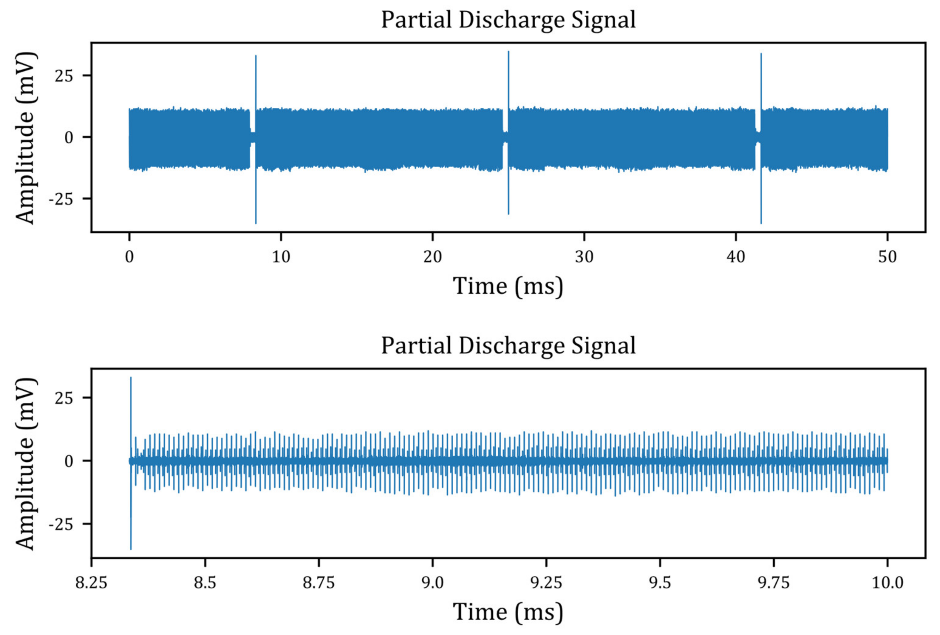Figure 7 shows an example of a signal collected in this region.

The aim was to assess the change in the partial discharge activity in different times of the day, considering the weather differences, such as temperature, humidity and wind direction—which is known to bring more or less sea salt in suspension from the ocean. Only measurements with the RF sensor were carried out. The pattern of pulses observed in the first structure was very similar to the pattern observed in laboratory when using the rigid wire and spark gap method: a few well defined pulses with low density, in specific regions of the power frequency cycle. The second structure presented a much higher density of pulses (higher repetition rate) during nighttime in comparison with daytime. The reason for this behavior is the higher relative humidity associated with the cooling of the insulator surface after the sunset, which may cause water condensation along the insulator surface.

By changing the acquisition window in the PicoScope software, it was possible to observe the pulses individually in detail, from which it could be observed that there was no difference in the pulse magnitude between day- and nighttime measurements. The higher the surface salt pollution and the relative humidity, the higher the number of PD pulses and the repetition rate. Finally, the third and last inspected structure presented the highest and most severe partial discharge activity out of the inspections carried out in the month of September, where the pulses were densely distributed along almost the entire cycle of the power frequency.

Another region of the city which could possibly be critical is the cargo port, since it is a site for the boarding of iron ore for the mining industry, and the insulators of that region constantly become covered in mine dust, as well as all structures and buildings in the surrounding area of the port, which constantly present a visible reddish dust deposit. Partial discharges were detected by the RF sensor and by the HFCT, since, in this case, the inspected structure had its grounding conductor exposed. However, the PD activity observed in the surrounding area of the port was not so severe as that observed in the previous region. Figure 8 shows the general layout of the concrete structures, and some of the insulators used in the utility’s system.

All the results presented in this last wave of tests confirm what has been stated in the previous section of this article and is stated in the literature: the pulse repetition rate and the interval between those pulses are good indicators of the partial discharge severity degree and, therefore, of the insulator pollution condition, regardless of amplitude, system calibration or relative positioning of the sensor in the field. In addition to that, it was realized that the HFCT would not be suitable for the system in question, given the inaccessibility of the grounding conductor in most of the structures inspected in the utility’s service area. Therefore, the RF antenna was chosen as the sensor to be used in this work.

3.3. Project of the Radiofrequency Sensor

Once the radiofrequency antenna has been chosen as the main sensor to be used with the proposed portable instrument, a log-periodic dipole array (LPDA) antenna was designed seeking robustness and compactness to make field operation more convenient. The design and equations were adapted from [30]. A crisscross connection of the dipoles was adopted. The specifications of the developed LPDA are:

• Operating band: from 500 MHz to 800 MHz
• Gain: 7 dB
• Impedance: 50 Ω

Initially, the operating band $\mathrm{B}$ is calculated:

$$\mathrm{B}=\frac{{\mathrm{f}}_{\mathrm{n}}}{{\mathrm{f}}_1}=\frac{800\mathrm{MHz}}{500\mathrm{MHz}}=1.6$$

(10)

Considering the desired gain and an LPDA gain curves graph, two parameters are determined: the spacing factor ($\mathsf{\sigma }$) and the scaling factor ($\mathsf{\tau }$). From the graph:

$$\mathsf{\sigma }=0.18$$

$$\mathsf{\tau }=0.86$$

From which, the antenna apex angle can be calculated:

$$\cot \mathsf{\alpha }=\frac{4\mathsf{\sigma }}{1-\mathsf{\tau }}$$

(11)

$$\cot \mathsf{\alpha }=5.14$$

$$\mathsf{\alpha }=11°$$

The band of the active region is then calculated:

$${\mathrm{B}}_{\mathrm{AR}}=1.1+7.7{\left(1-\mathsf{\tau }\right)}^2\cot \mathsf{\alpha }$$

(12)

$${\mathrm{B}}_{\mathrm{AR}}=1.88$$

From which, the bandwidth of the antenna can be calculated:

$${\mathrm{B}}_{\mathrm{S}}=\mathrm{B}·{\mathrm{B}}_{\mathrm{AR}}$$

(13)

$${\mathrm{B}}_{\mathrm{S}}=3.00$$

Based on these parameters, the dimensions of the antenna can be determined. The maximum wavelength is given by:

$${\mathsf{\lambda }}_{\mathrm{MAX}}=\frac{3·{10}^8\mathrm{m}/\mathrm{s}}{{\mathrm{f}}_1}$$

(14)

$${\mathsf{\lambda }}_{\mathrm{MAX}}=0.06\mathrm{m}$$

Then the length of the support boom is calculated:

$${\mathrm{L}}_{\mathrm{BOOM}}=\left(1-\frac{1}{{\mathrm{B}}_{\mathrm{S}}}\right)\cot \left(\mathsf{\alpha }\right)\frac{{\mathsf{\lambda }}_{\mathrm{MAX}}}{4}$$

(15)

$${\mathrm{L}}_{\mathrm{BOOM}}=0.51\mathrm{m}$$

The length of the longest dipole element is given by:

$${\mathrm{l}}_1=\frac{149.96·{10}^6}{{\mathrm{f}}_1}$$

(16)

$${\mathrm{l}}_1=0.30\mathrm{m}$$

Finally, the number of dipoles is calculated:

$$\mathrm{N}=1+\frac{\log {\mathrm{B}}_{\mathrm{S}}}{\log (1/\mathsf{\tau })}$$

(17)

$$\mathrm{N}\cong 8$$

Once determined, the length of the longest dipole can be used to calculate the other elements.

$${\mathrm{l}}_{\mathrm{n}}=\mathsf{\tau }·{\mathrm{l}}_{\mathrm{n}-1}$$

(18)

The distance between the first two dipoles is given by:

$${\mathrm{d}}_{1–2}=\frac{\left({\mathrm{l}}_1-{\mathrm{l}}_2\right)\cot \mathsf{\alpha }}{2}$$

(19)

$${\mathrm{d}}_{1–2}=108\mathrm{mm}$$

The other distances can be calculated by:

$${\mathrm{d}}_{\left(\mathrm{n}-1\right)-\mathrm{n}}=\mathsf{\tau }·{\mathrm{d}}_{\left(\mathrm{n}-2\right) -\left(\mathrm{n}-1\right)}$$

(20)

The final specifications of the antenna, regarding dipoles sizes and their distances between each other are shown in

Table 3. Dimensions of each dipole element.

Dipole Element	Dipole Length (mm)	Dipole Half-Length (mm)	Distance from Previous Dipole (mm)
1	300	150	-
2	258	129	108
3	222	111	92
4	190	95	80
5	164	82	68
6	142	71	60
7	122	61	50
8	104	52	44

.

Eight antenna prototypes were initially built and then validated by means of laboratory tests. The results were compared with the performance of the antenna of Model 242 and demonstrated that the antenna that was designed is suitable for the application of this work. The antenna that was built is shown in Figure 9.

3.4. Laboratory Tests for the Evaluation of the Performance of the Algorithms

After the implementation of the algorithms has been completed and the partial discharge sensor has been chosen and designed, the proposed portable instrument was assembled. The first version of the instrument was initially assembled using a Raspberry Pi 3B+ as its core (which was later updated to model 4B with 4 GB of memory) to which a PicoScope oscilloscope and a touch screen display were connected to. The PicoScope is used to collect the data to be analyzed by the algorithms, whereas the touch screen display provides access to the system for the user.

The algorithms of data acquisition and analysis work as modules which must be called by a main process. Therefore, in order to provide an interface for the user and call the algorithms to perform the required actions, a web-based software was developed to run on the Raspberry Pi operational system, Raspberry Pi OS (previously called Raspbian) based on Debian 10. The front end of the software was implemented using HTML, CSS and JavaScript, whereas the backend was implemented in Python language. The software provides access to the general settings of the instrument, such as documentation, insertion and deletion of users, transmission lines, and georeferenced structures, and also to the data acquisition and analysis algorithms.

The system power is supplied by a rechargeable battery, which is connected to an energy management circuit. This circuit is responsible for controlling the power supplied to the components and the battery charge. All these pieces of equipment are placed inside a protective equipment case provided with a panel comprising the touch screen display, a power switch, the AC power connector, a USB connector to collect data, and a BNC connector to which the antenna is attached to at the time of the inspection. The assembled portable instrument (portable software-hardware system) is shown in Figure 10.

To perform a field inspection at a structure using the portable instrument, the user shall select the desired settings, and run the inspection software while pointing the antenna at the direction of the desired structure. After the data acquisition, the instrument processes and analyzes the signal content. The instant result indicates whether partial discharges are occurring at the structure, and, if so, the activity severity degree. The full results are saved as a PDF file, which can be later exported to a flash drive.

Thus, once assembled, the final portable instrument had to be tested in laboratory prior to delivery to the electric utility. These final laboratory tests would serve as an evaluation and validation step both for the portable instrument (hardware and software) and the severity degree. The main concern was how a laboratory test could faithfully reproduce the pollution to which insulators are subjected in the environment of the utility’s service area. Following the recommendations of the solid layer method pollution test prescribed by IEC, kaolin was used to make the tests feasible. However, it was desired to use actual pollution degree data from the utility’s service area, whose quantity can be measured by the equivalent salt deposit density (ESDD), i.e., the amount of NaCl per area of the insulator surface which, when dissolved in water, will produce the same conductivity as that of the natural occurring pollution layer.

Monteiro Porfírio [31] carried out a study regarding the effects of weathering on high voltage insulators, which resulted in her doctoral thesis, whose case study analyzed the same city of this work. The city of São Luís is located on an island close to the Equator, with a tropical climate, being October its driest month with a precipitation of 7 mm. The average temperature only varies about 1.4 °C over the course of the year, but the dry and the rainy seasons are noticeable prominent, e.g., comparing October with May, which presents a precipitation of 367 mm [32].

The study described in [31] used four tube collectors with longitudinal slits, each of them facing a cardinal direction, placed onto poles at the desired sites. The deposit of pollutants collected inside the tubes was then dissolved in water and filtered next. The composition of the pollutants was split into soluble and non-soluble materials from which the solution containing soluble materials had its conductivity measured in µS/cm. This quantity was then converted to ESDD values, measured in mg/m² day, considering the volume of water used, the area of the tube slit, and the collection period. The obtained value of ESDD corresponds to the amount of NaCl that, if dissolved in water, would result in the same conductivity as that of the pollutants soluble content.

Therefore, considering the ESDD values obtained by the study mentioned above [31] as reference, and considering the surface area of the samples of polymeric line post insulator to be tested in the work described in this article, some amounts of NaCl were selected to be used in the solid layer method of artificial pollution test recommended by IEC 60507:2000. The cumulative values of the ESDD for the period Jul-Oct and for the month of October were considered from which the respective amounts of NaCl were calculated, and from which, in turn, partial amounts of NaCl were calculated, corresponding to partial time periods within the dry season, as shown in

Table 4. Equivalent salt deposit density for each period and the respective amounts of NaCl.

Period	ESDD (mg/cm2)	NaCl Amount (g)
July–October	0.614	9.48
50% July–October	-	4.74
October	0.197	3.05
50% October	-	1.52
25% October	-	0.76

.

The partial-month periods seek to determine an approximation of week periods of pollution. This was done considering the need for the electric utility maintenance team to perform insulator washing every week during the months of highest pollution deposition. This frequency of washing is considered remarkably high in comparison with other electric utilities located in different regions of the country. Each amount of salt mentioned in Table 4 was first dissolved in 61.1 g of water, and an amount of 67.2 g of kaolin was added next, resulting in a slurry in enough amount to cover the entire surface of the sample, including metal fittings and underneath weathersheds.

The slurry was applied to the samples using a paint brush, and the samples were left to dry naturally next. Once dry, the sample to be tested was placed inside the chamber and the fog generators were turned on until the relative humidity inside the chamber reached more than 85% and the pollution layer was slightly wet. Next, the fog generators were turned off, and nominal voltage of 40 kV was applied to the sample. The partial discharge activity was monitored by means of the antenna (whose project and assembly are described in Section 3.3) and the PicoScope oscilloscope (using PicoScope software). The signals were acquired and saved for further analysis. The schematic and the actual experimental setup of this laboratory test are both shown in Figure 11.

The partial discharge activity pattern, i.e., the pulse density would lower according to the decrease of the relative humidity inside the chamber. It was also possible to observe the similarities between these signals and the patterns observed in the field from the naturally polluted insulators. After acquisition, the signals were subjected to analysis by the developed algorithms, aiming to assess their performance and the conformity of the proposed severity degree. Considering the solid layer with the corresponding pollution for the month of October, the severity degree as a function of humidity is shown in Figure 12.

As expected, the decrease in relative humidity inside the test chamber caused a decrease in the partial discharge activity, reflected by the severity degree generated. For relative humidity values under 70%, the severity degree decreased to values under 5 in most of the cases tested. The calibration of the FIS is based originally on the field collected signals, and a severity degree of 10 was assigned to the worst scenario observed. Severity degree values were also compared considering the different amounts of NaCl accounting for the different scenarios of pollution for each period considered. For the first two periods considered in Table 4, the fog generators were left on until a considerable amount condensation was observed on the test object surface, then nominal voltage was applied to it and the fog generators were turned off. A comparison for these two periods is shown in Figure 13. Only severity degree results for values of relative humidity above 70% were plotted, from which it is possible to notice a decrease in the median value (orange line) and in the mean value (green triangle) according to the decrease in the surface pollution, i.e., in the salt deposit.

In addition to that, considering the ESDD for the month of October, approximate time periods equivalent to two weeks (50% October) and one week (25% October) were considered by using the percentage amounts of NaCl. In this case, the fog generators were turned on for a short period, between 5 and 10 min, until the measured relative humidity inside the chamber reached a value around 85%, and then turned off before applying nominal voltage to the test object. The results of the severity degree for values of relative humidity above 70% for this case are shown in Figure 14.

Even though some decrease in the severity degree can be observed, by the median and mean values, from the October pollution level to the other two periods, the mean values for the pollution equivalent to two weeks and one week of October did not follow a decreasing behavior. Considering the little amount of salt used in these two cases, the ideal homogeneity of the deposit distribution on the test object surface may have not been reached, thus presenting the divergence observed. However, overall, individual results showed good correlation to the test conditions.

3.5. Offline Evaluation of Field Collected Data, and Calibration of the Severity Degree

Overall, the laboratory tests showed results that validate the performance of the algorithms and the consistency of the severity degree. After these laboratory tests, the data that had been collected in the field tests mentioned in Section 3.2 was subjected to an offline analysis by the algorithms. The results of this analysis should be compared to the reports from the utility’s team and the observations made during data acquisition in the utility’s service area. These data have been used to calibrate the FIS, and to generate the severity degree values presented next.

The first region considered comprises a group of transmission structures in the surrounding area of the utility’s headquarters. It is located around 2.5 km from the coastline. Even though the reports do not point this as a critical area, the field inspections performed showed a variety of very severe and moderate severe partial discharge activity. The average generated severity degree for one of the structures was 10, whereas for a second structure it ranged from 5 to 9, with an average of 7. This region is relatively close to the ocean, has wind continuously blowing, and is crossed by an important avenue. These conditions lead to moderate surface pollution conditions, which can be observed by the variations of the severity degree values.

Now considering the most critical region, located in the middle of the island, as mentioned before, three different structures had been inspected. The first structure had been inspected only during the day. In Figure 15, it shows that this structure presented a mildly severe partial discharge activity, with an average severity degree of 3. The second structure, which had been inspected during the end of the day and beginning of nighttime, showed a clear difference between the PD activity during these two time periods.

Considering the working hours of the utility’s team, the FIS should be calibrated to generate the maximum severity degree for the worst condition observed during daytime. This means that worse conditions observed during nighttime should be assigned a severity degree of 10. This behavior can be observed in Figure 15, especially regarding the second structure, which had been inspected both during daytime and nighttime. The third and most critical structure with respect to PD activity had been inspected only during nighttime, and presented visible arcing, also confirmed by the residents of that region. Therefore, for this last case, all data samples produced a severity degree of 10.

Considering the third region that had been inspected, the structures are located between another important avenue and an area of mangroves. During field data collection, no discharge pulses had been detected with the antenna or the HFCT. Instead, a variety of telecommunication signals had been collected. For this case, the neural network assigned these signals the “not recognized” class, resulting in a severity degree of 0. Finally, the last region where field data had been collected from is the cargo port region. Even though some visible surface pollution was visible because of the mining activities, the signals from this region had not shown particularly recognizable partial discharge activity, which was confirmed by the algorithms, which assigned these signals to the “not recognized” class.

Therefore, given the consistent results generated by the algorithms when compared with the field observations, the portable instrument is expected to be helpful for the utility’s team when inspecting the structures in their service area during the dry season, serving as an important decision support tool.

4. Discussion

The partial discharge severity degree obtained from the portable instrument proposed in this work will allow the electric utility to have an additional decision support tool for the inspection of high voltage insulators in their system. Thus, this instrument provides guidance and confidence about the real condition of the structures through a straightforward diagnosis that enables any person to perform the inspection. Inspections are usually uncertain, relying on experts to perform them. The instrument, in turn, provides assurance for any person. By combining the history of the structure under inspection with the results provided by the instrument, maintenance actions can be directly scheduled, such as washing or replacement. Therefore, costly maintenance routines can be oriented to structures that really need cleaning or replacement, rather than randomly performing these routines to prevent failures.

Today, the main method of prevention of system failures due to surface discharges is insulator washing. This is a costly method that is performed considering observations made by experts, and the history of the structure. However, with the help of the instrument proposed in this work, the maintenance personnel will have an additional decision support tool to assess the real condition and decide whether or not insulator washing should really be performed. This represent cost savings from the point of view of maintenance expenses. Still considering insulator washing, not all structures can be covered with this preventive maintenance routine when inspection is carried out with traditional inspection methods, which often results in flashovers and system failures in the most degraded structures. With the help of the proposed instrument, a larger number of structures can be inspected and assessed, reducing corrective maintenance costs and fines for power outages.

Considering the proposed laboratory test methodology, it demonstrated its capability to reproduce the field conditions based on real data obtained from the referenced work. The use of a denser suspension of kaolin and sodium chloride enables the solid layer test method to be used with polymeric insulators, despite its hydrophobicity. In addition to that, the selected parameters for calculating the severity degree show the possibility of using relative parameters instead of absolute magnitude and apparent charge quantities.

Regarding the instrument itself, the use of an antenna enables it to be used not only at high voltage insulators, but also with other equipment which may present partial discharges. The most obvious limitation lies on the data size involved in the acquisition and analysis processes, which can be a constraint, given the use of a Raspberry Pi as the processing unit. However, the update of the Raspberry Pi model used, which resulted in a memory update, enhanced the processing capability and performance, enabling the acquisition of a list of signals to be analyzed individually, increasing the results accuracy.

5. Conclusions

To summarize the results, the algorithms and the proposed severity degree have been validated through laboratory and field tests, showing a consistent correlation between the partial discharge activity and the severity degree. This validation can be confirmed when different levels of pollution are used in the laboratory, and their effect on the partial discharge activity is demonstrated by the severity degree. Thus, the hypothesis defined in the Introduction of this article can be confirmed, i.e., the pollution degree is correlated to the partial discharge activity in this case study.

In terms of contributions, this article brings a methodology focused on the online inspection of high voltage insulators. To achieve that, the use of a LPDA antenna was proposed as a non-intrusive sensor that can be used in field inspections while maintaining safe distance of the high voltage apparatus. The results have shown that its use in the detection of partial discharges is efficient and adequate for this type of detection.

Another contribution that can be highlighted is the use of parameters that are not dependent of magnitude or apparent charge for the assessment of the partial discharge activity. This method also allows the evaluation of the condition of insulators without the need for long term monitoring, since the proposed severity degree is calculated instantly regardless of past events.

In addition to that, overall contributions have been made regarding the use of convolutional networks and fuzzy logic in applications of electric power systems. This type of study still endures today, because there are still several aspects that can be explored as these artificial intelligence tools evolve.