3.1.1. Quantity and Quality of the Biogas Produced before/after the Separation of Starch and Mango Seed Coats
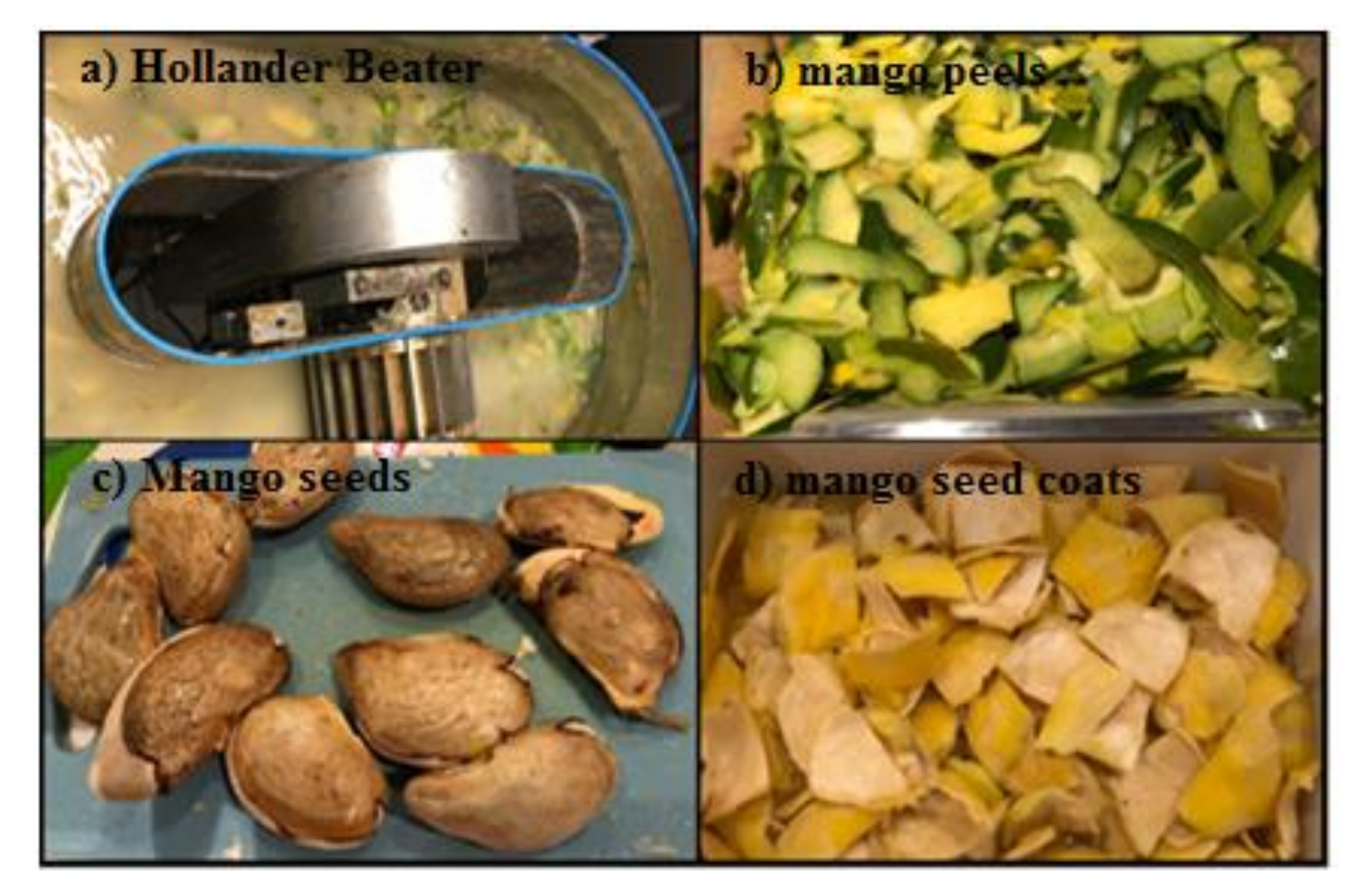
The weights of all main mango wastes were measured separately. The results of the measurements revealed that mango wastes represent approximately one third of the total weight of the mango. This finding is in accordance with O’Shea et al. who stated that between 35–60% of the total mango weight is discarded after processing. The weights of the peels, seed and seed coats were 90, 25, 30 g per mango, respectively. This means that, the seed represents approximately 18% of the total weight of the mango waste. The starch weight was also measured and found to constitute 4 ± 1% of the total weight of the mango waste and 19 ± 2% of the seed weight. This finding is in accordance with Saadany et al. [
23]. As previously described, the starch was only included in the controls along with whole mango wastes and excluded from the other reactors.
Table 4 illustrates the general results of the AD of mango wastes after the separation of starch and coats. The table also includes the pH levels of each run after the digestion process. To simplify the comparison of the results and obtain more accurate results, the organic concentration g-VS of the controls were set to the highest concentration (6.5 g-VS).
Table 5 shows the differences between the results of the controls and the predicted results of the biogas produced from the mango wastes after the separation of starch and coats at 6.5 g-VS and 50% sludge at the three temperature levels.
According to
Table 4 and
Table 5, the pH levels of the controls and all runs were in the range of 6.5 to 8. This indicates the equilibrium of the systems and the stability of all digesters. It worth also noting that, prior to feeding the digesters, the pH of the sludge was measured and found equal to 7.9 ± 1. From
Table 4, a relationship between the VS concentration (B), sludge concentration (C) and the pH level can be observed. Therefore, the pH level decrease as the organic concentration increases and the sludge concentration decreases. In regards to the volume of the biogas produced from the one g-VS, the highest was found at 35 °C (A), 1.6 g-VS (B) and 50% (C). While, the lowest was obtained at 35 °C (A), 6.5 g-VS (B) and 20% (C). On the other hand, the largest CH
4% was found at the centre point and was 68.9%. Run 2 which has recorded the lowest biogas volume/g-VS has also recorded the greatest level of CO
2 (61%).
In reference to
Table 5, it is clear that the incorporation of the starch and coats negatively influenced the biogas quantity, while, its influence on the quality of the biogas was also negative but less than its influence on the biogas quantity. As the starch weight were relatively low in the controls compared to the total weight of the waste, this finding can be mainly attributed to the stiffness of the mango seed coats. Therefore, they were difficult to digest by the microorganism.
The followings show the analysis of each response separately. They were carried out using the DOE. Each analysis of response, provides a statistical analysis of the developed model, measures the adequacy of the model, depicts the behaviour of each factor on the response and shows the significant influences of each factor and their interactions (if any) on the response.
- (1)
Biogas volume per each gram-VS
In the proposed study, if the
p-value of the model and of any term does not exceed the level of significance (α = 0.05), they are considered statistically significant within the confidence interval of (1 − α).
Table 6 show the ANOVA analysis generated by Box-Behnken design (BBD) as a RSM approach for the biogas volume produced from one gram-VS of the mango waste after the separation of the starch and coats. The analysis has proven that the model was significant, the lack of fit was insignificant and the regression was good. It has also illustrated that the coded model terms: A, B, C, A
2 and C
2 had significant impacts on the biogas yield produced from each g-VS. It can be observed from the analysis also that, C (%) has the most significant influence, following by the influence of the B (g-VS). While, the influence of A (°C) was less significant than the influences of the other factors.
Equation (8) illustrates the final mathematical equation in terms of actual factors as obtained by ANOVA for biogas volume/g-VS:
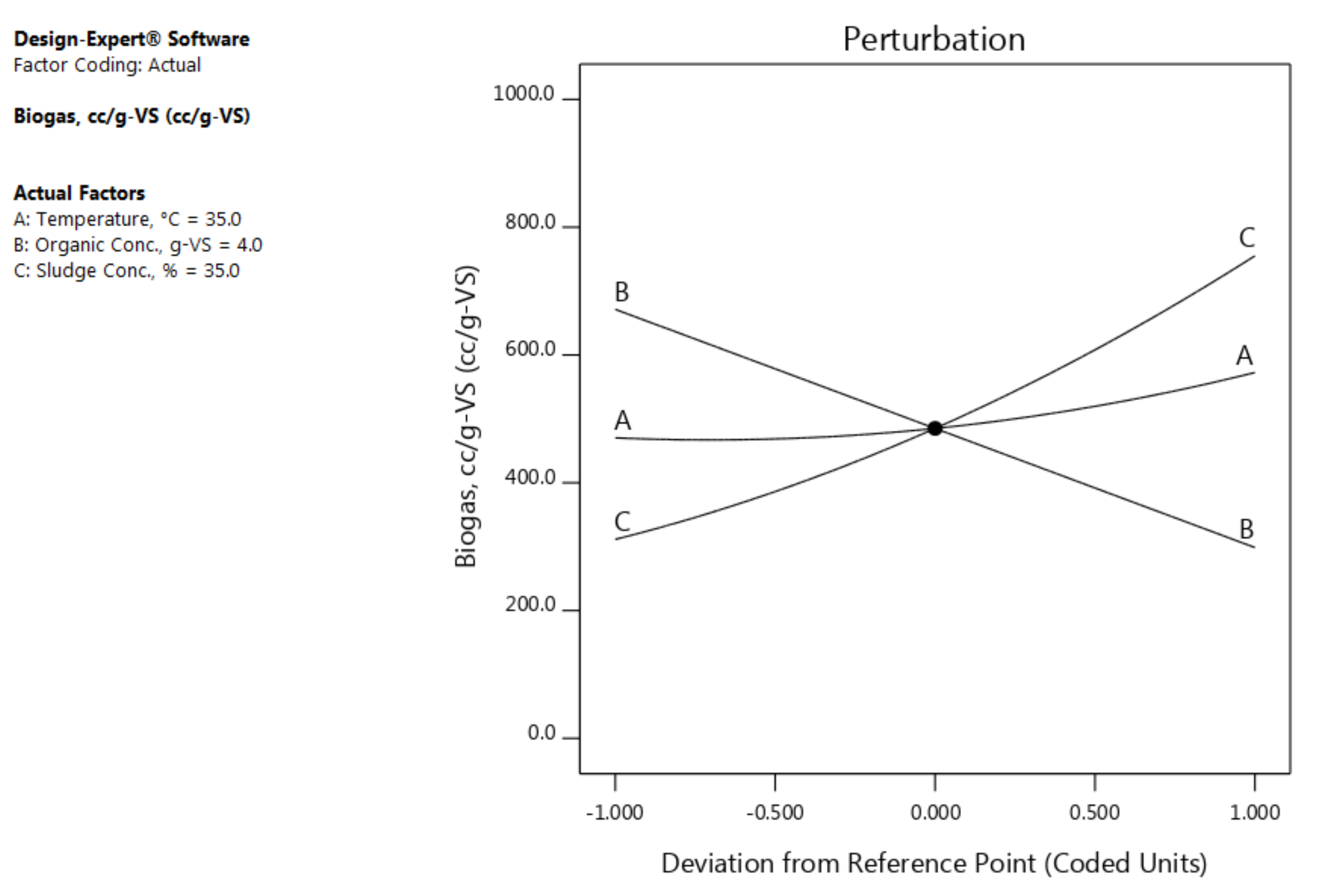
The perturbation plot (
Figure 2) illustrates the behaviour of each factor on the response. As it can be noted, the temperature (A) has a slight positive influence on the volume. However, increasing the organic concentration (B) decreases the biogas volume. It is also clear that, the sludge concentration (C) is in direct proportion with the biogas volume produced from g-VS.
The ANOVA analysis of the CH
4% is given in
Table 7 and depicts that the developed model and the lack of fit were significant. It also shows that the model terms A, B, C, BC, B
2 and C
2 have significant influences on the CH
4%. The “Adeq. Precision” as one of the adequacy measurement tools was greater than 4, therefore, the model can be used to navigate the design space.
In addition, the actual mathematical model resulted from this response is illustrated in Equation (9):
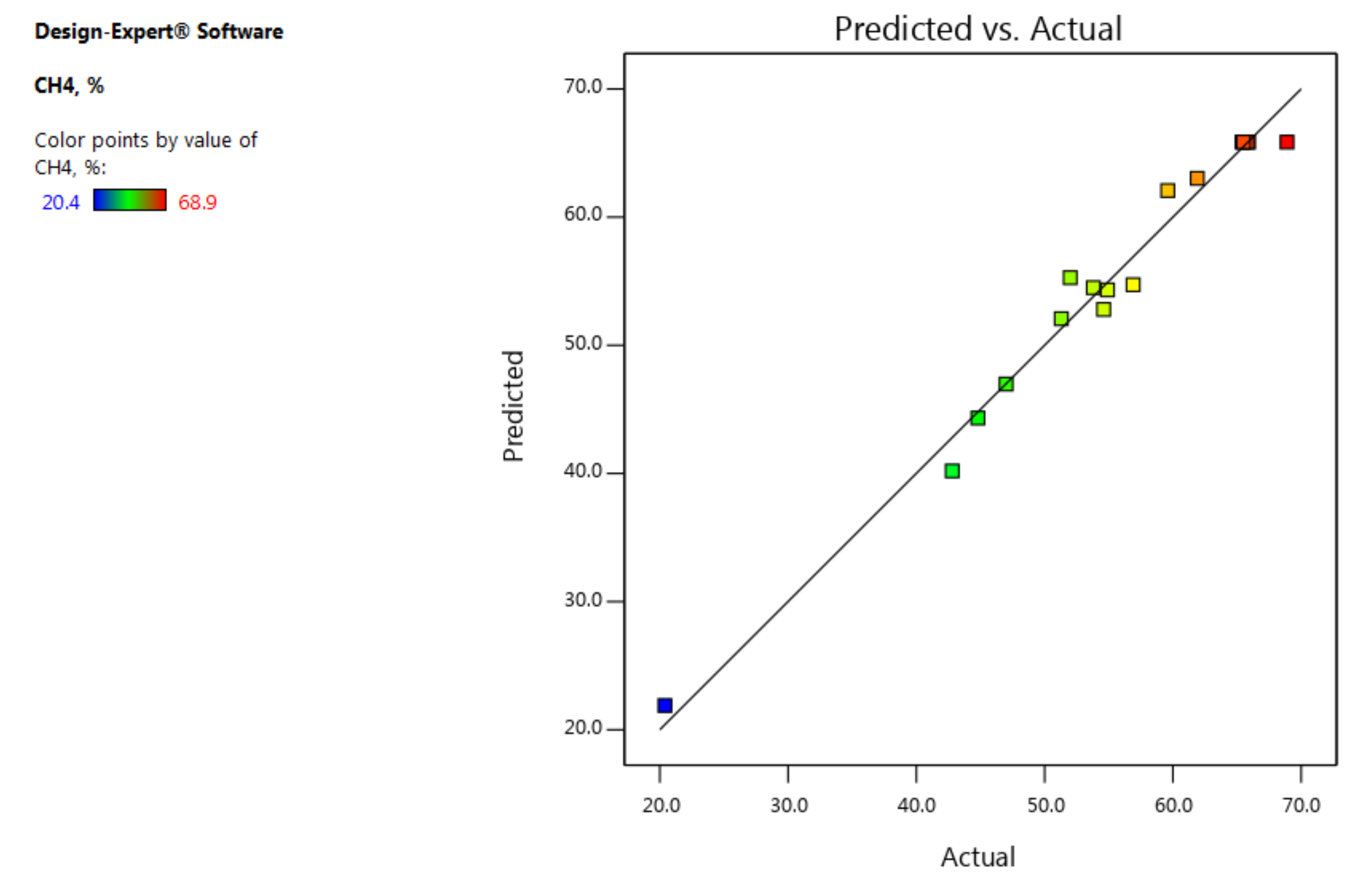
Moreover,
Figure 3 shows the predicted results versus the actual results plot. The plot helps in validating the strength of the generated model and shows the correlation between the actual and predicted response values. The distribution of most of the points in
Figure 3 on the diagonal line or closer to it implies that, the model predicted the results very well and thus, there was a good correlation between the model’s predicted results and the actual ones.
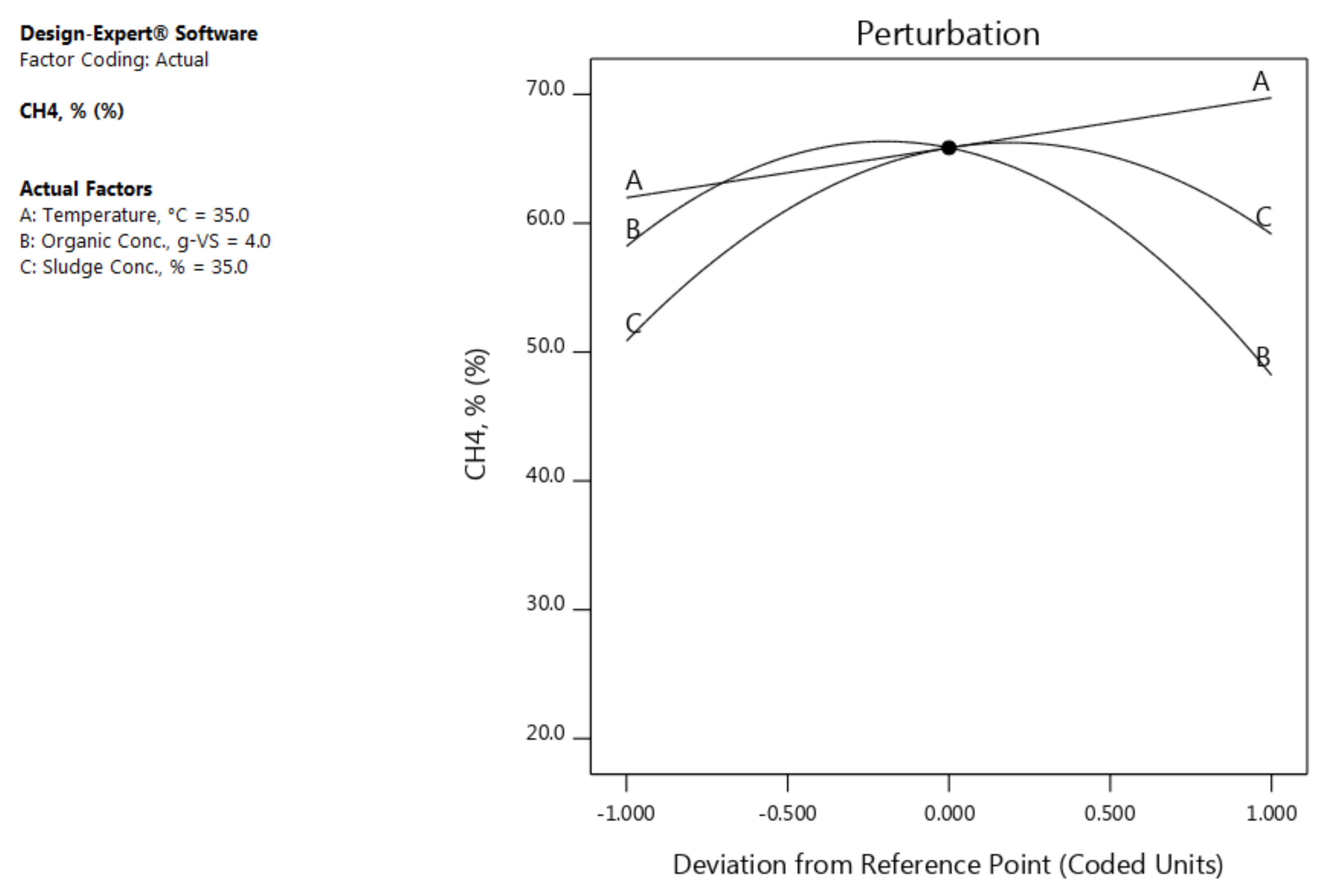
According to the perturbation plot in
Figure 4, the CH
4% increases as the temperature increases in the studied range. While, it is increases as the organic concentration (B) increases until it is reaches just before the reference point (4.05 g-VS) and begins to decline gradually. In terms of the sludge concentration (C) influence, the CH
4% increased as the concentration of the sludge increased until the concentration of the sludge reached approximately 40% and then the CH
4% started to decrease slightly.
The interaction and contour plots are provided to illustrate the influences of the interactions of the factors.
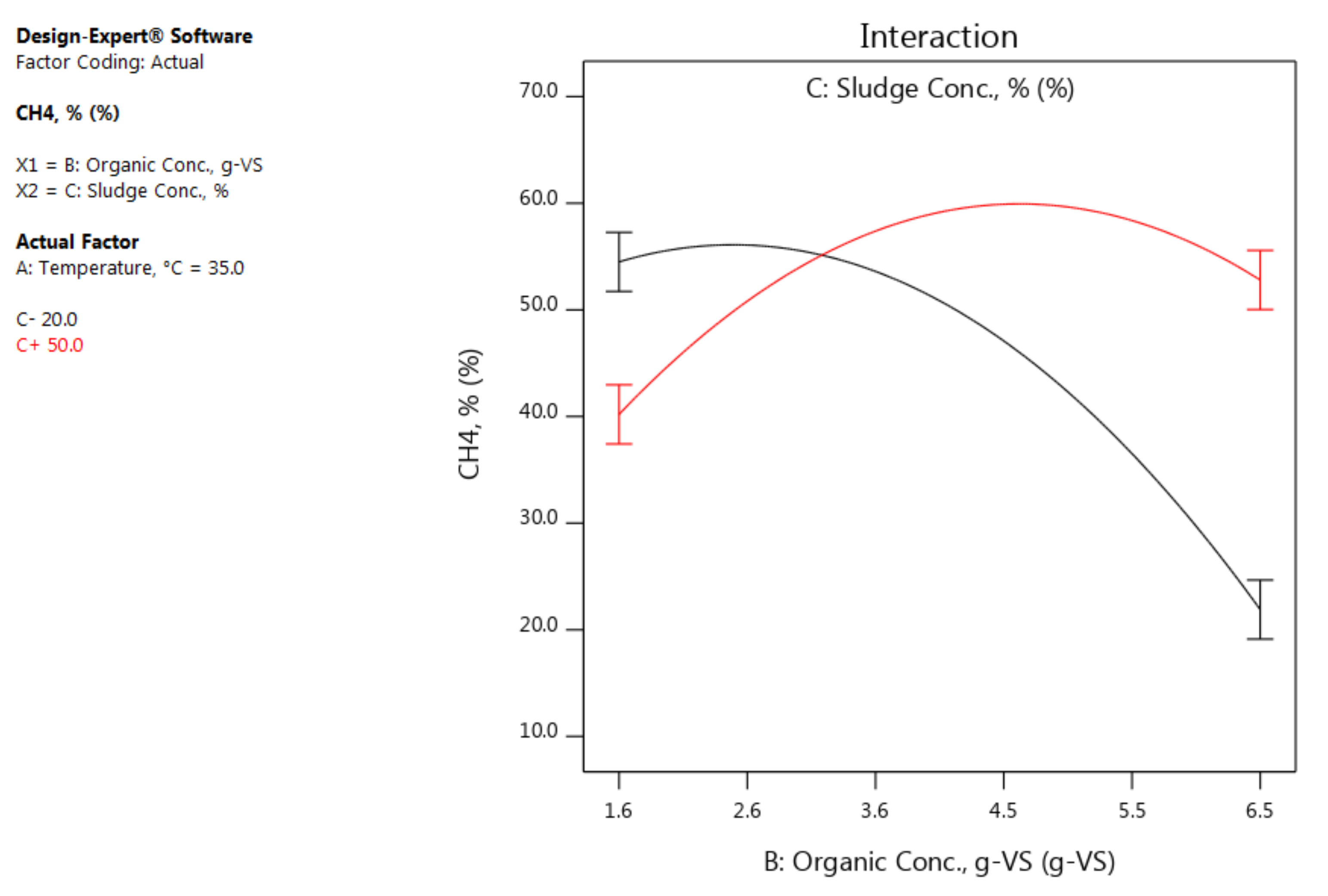
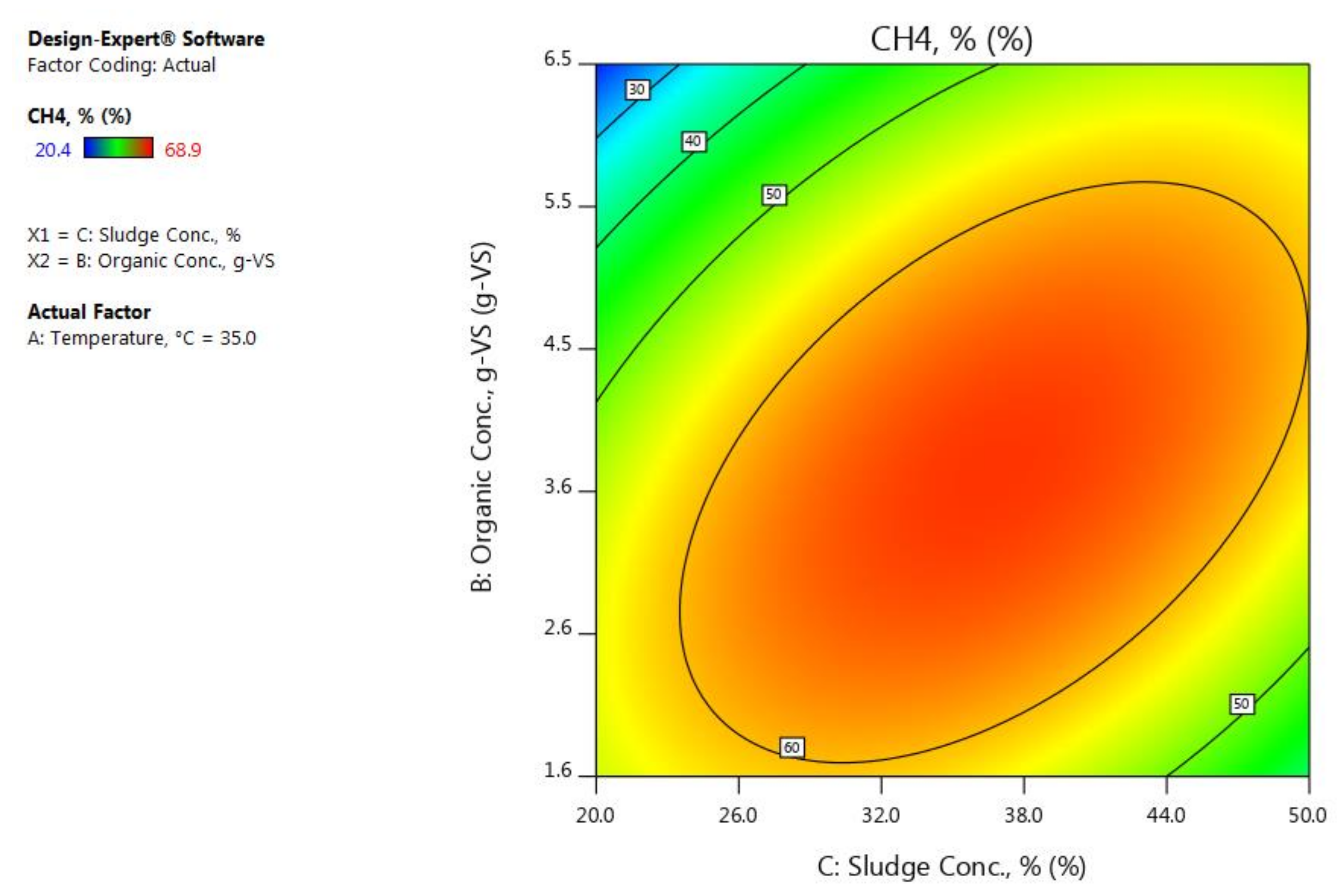
Figure 5 and
Figure 6 show the interaction and contour plots of the influence of the interaction of the organic concentration and sludge concentration on the CH
4%. It is obvious that, when the organic concentration is at the lowest level, changing in the sludge concentration does not make a big difference on the CH
4%, but when the organic concentration is at the highest level, a significant variation in the CH
4% can be observed when the sludge concentration is increased or decreased. In addition, when the sludge concentration is kept at the lowest level and the organic concentration increases in the studied range, thus the CH
4% stays at approximately a constant level and then remarkably decreases after the organic concentration has reaching approximately 2.8 g-VS.
- (3)
Carbon dioxide concentration
The results of the ANOVA analysis of the developed model which was generated based on the CO
2% has confirmed that the validity of the model was significant and found the “lack of fit” to be insignificant (see
Table 8). It worth noting that, the CH
4% and CO
2% responses were significantly influenced by the same terms. The analysis has also proved that the “Adeq. Precision” of the model was greater than 4 and therefore the model can be used to navigate the design space. It was also shown that the regression of the model was good as the R
2, adj. R
2, and pred R
2 were all close to 1 and the “pred R
2” of 0.89 was in reasonable agreement with the “adj. R
2” of 0.96.
Equation (10) shows the actual mathematical model of this response according to the ANOVA:
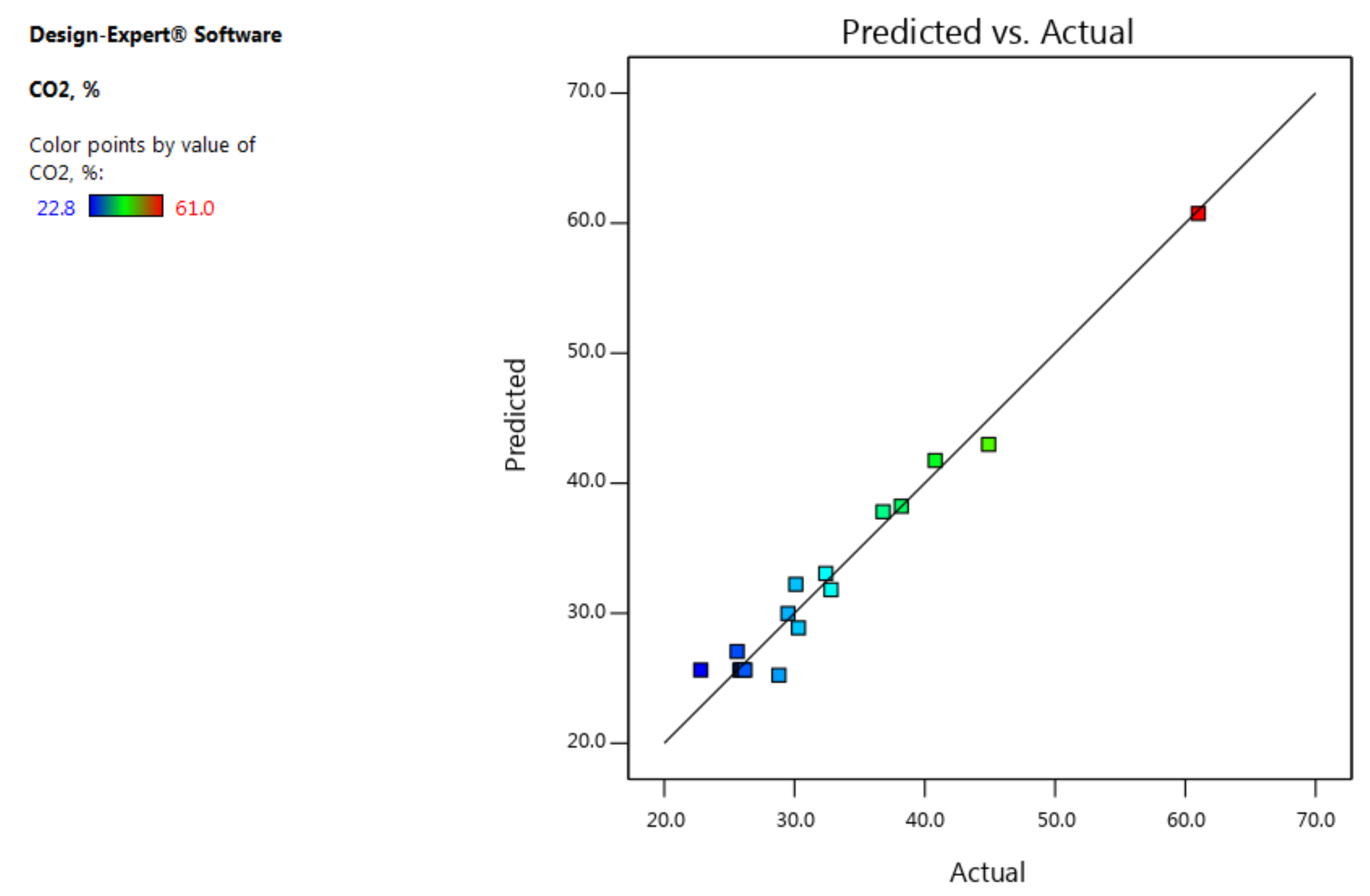
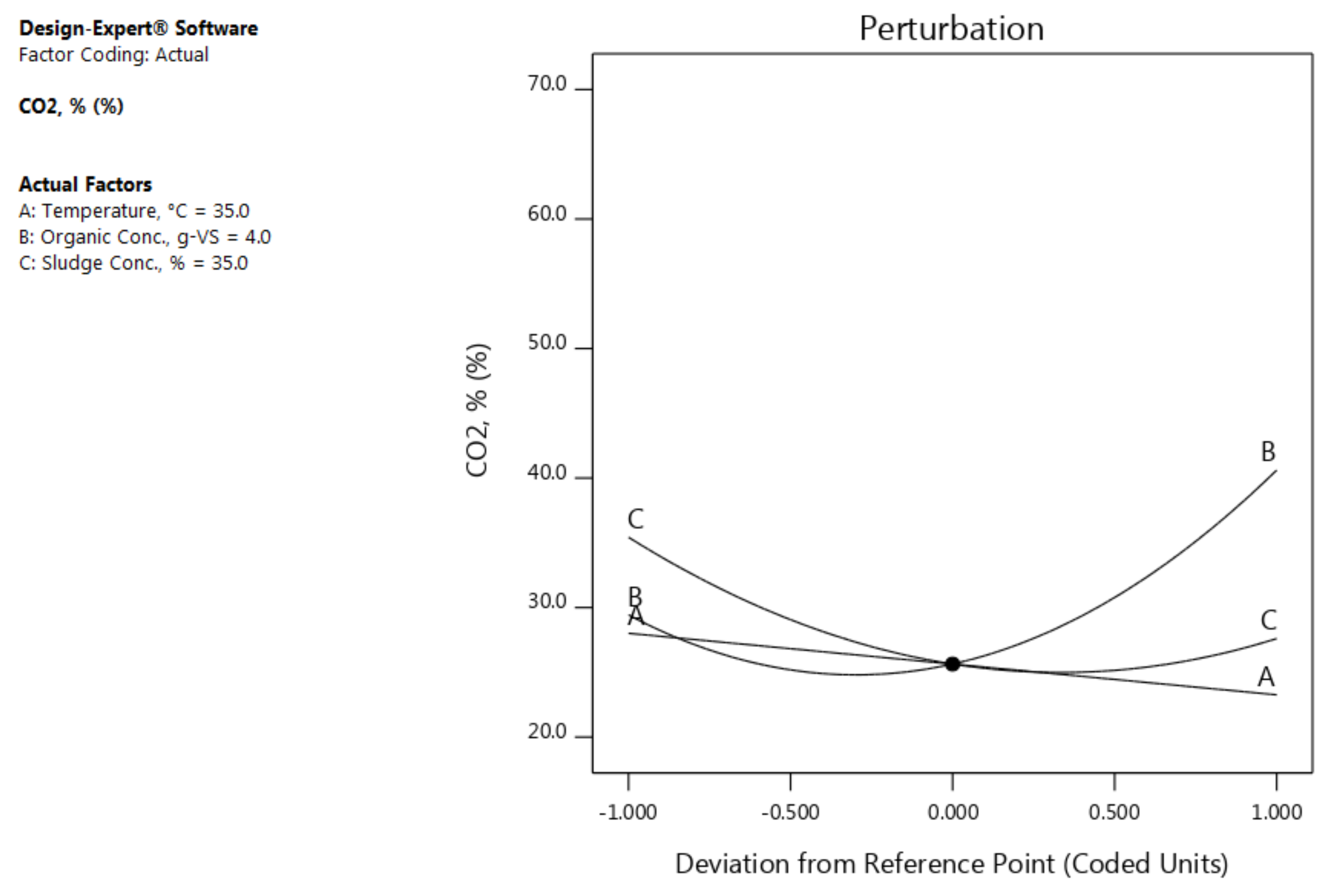
Figure 7 indicates that, there was a reasonable correlation between the model’s predicted results and the actual ones. The perturbation plot (
Figure 8) has also shown that the behaviours of all factors with the CO
2% are almost opposite to the behaviours found for the CH
4%.
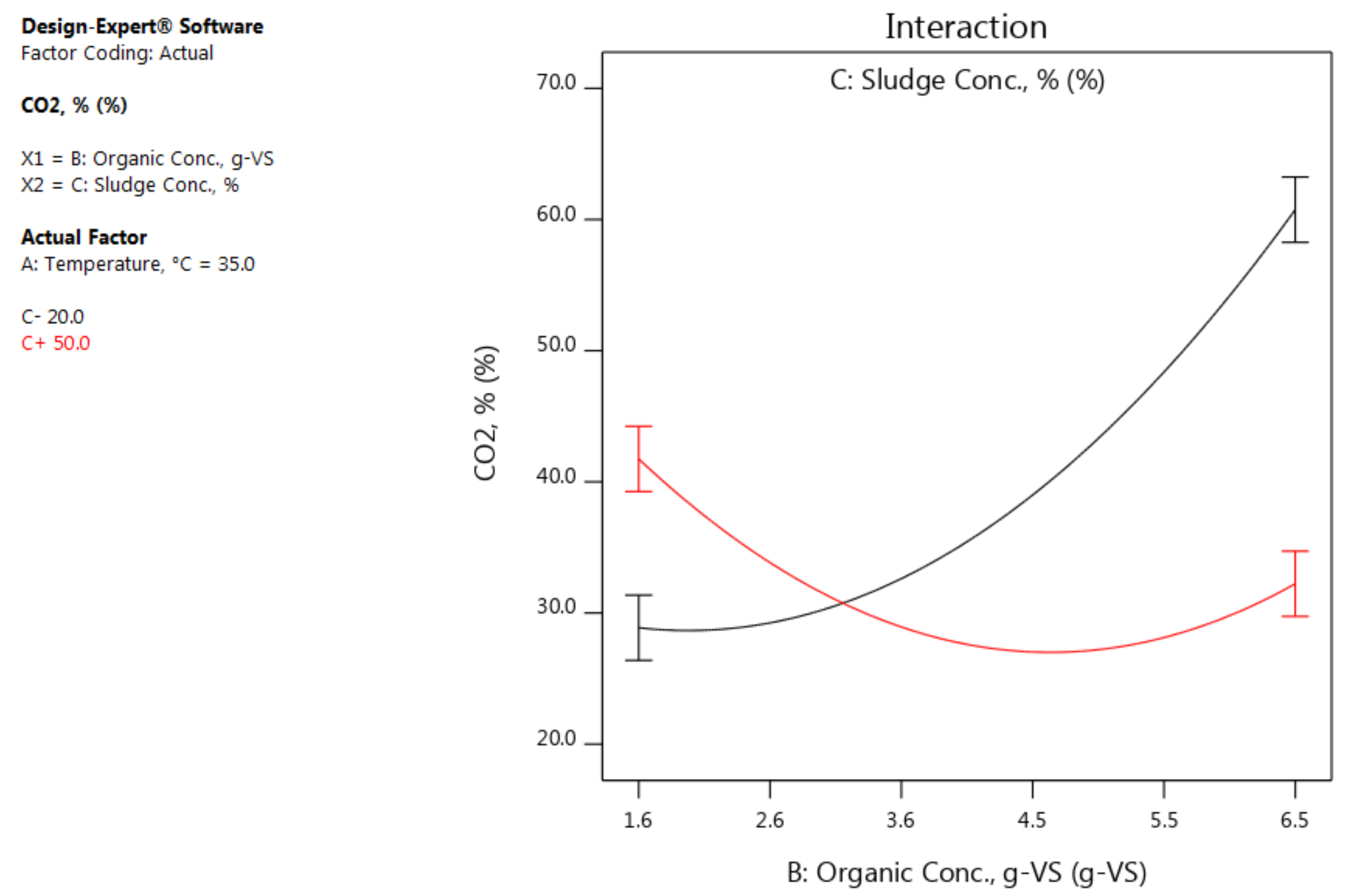
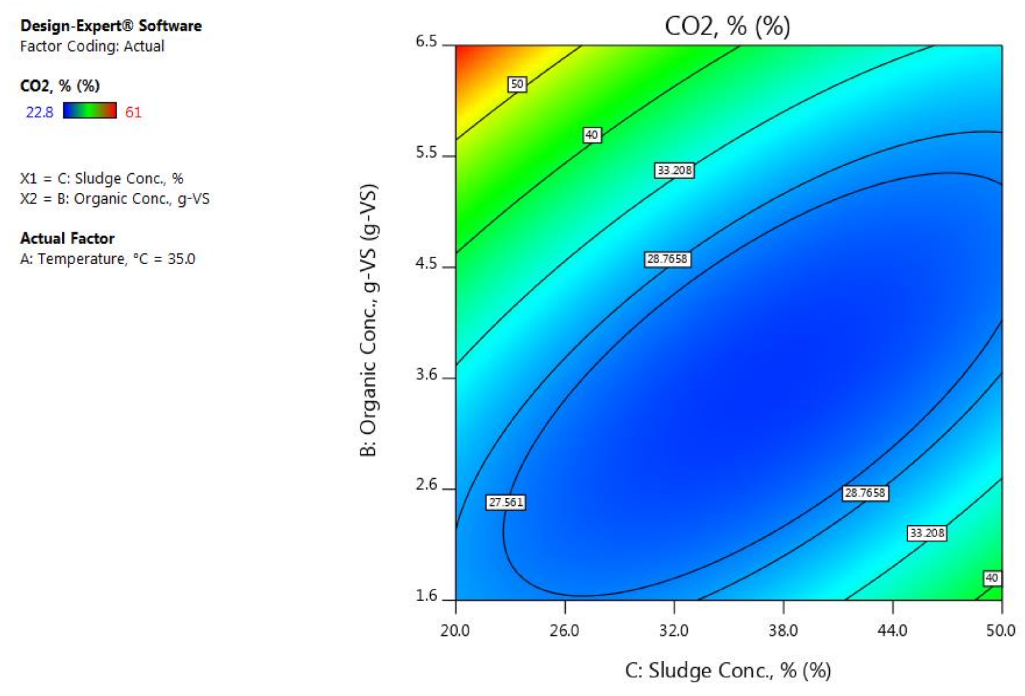
Relatively, the same concept of the influence of the (BC) on CH
4% is applicable to its effect on the CO
2% but in an opposite manner. For instance, when the organic concentration is at the highest level, a significant variation in the CO
2% can be observed when the sludge concentration is moves from its lowest to its highest levels (see
Figure 9 and
Figure 10). However, based on the analysis of the CO
2% response and by looking back into the analysis of the CH
4% response, the same terms have a significant effect on both responses but to varying degrees. In comparison between the results of the concentrations of both CH
4% and CO
2% which have been measured from each run, it is evident that the increase in CH
4% is associated with a decrease in CO
2% and vice versa.


