Abstract
Usually thermal response tests are restricted to big geothermal projects; the high investment makes them less suitable for designing domestic low-enthalpy geothermal energy systems. The work here presented aims to study the influence of time reduction in thermal response tests on their precision. Due to the importance of the correct assessment of the thermal characterization of the ground for any kind of geothermal system, time reduction in this essay could make it more affordable to be implemented in some domestic systems. A thermal response test has been implemented, and several time intervals of the test have been considered in order to obtain different results for the thermal conductivity of the ground. The mentioned results have been then compared and also the domestic geothermal systems designed from them by the use of the geothermal software GES-CAL. Results have shown that, in some cases (our testing borehole has some singular characteristics), a significant time reduction in the data acquisition process of the thermal response test does not compromise seriously the precision of the results.
1. Introduction
The design process of low-enthalpy geothermal systems has undergone a continuous improvement process in the last few years [1,2,3,4]. From the correct assessment of the thermal needs to the selection of the heat pump or the design of the bore field, all of the key areas of the future system are improving at a fast rate nowadays. Geothermal heat pumps are subjected to more exhaustive control than ever in both their performance statements and their ranges of use [5], the coefficients of performance are improving, and the diversification of new models to satisfy more and more variety of needs is a fact. However, ground characterization remains relatively underdeveloped for small domestic systems because of the high cost of the tests needed to be implemented, restricting the data collecting about ground thermal behavior to the research of databases [6] and the bibliographic study of the geological environment of the area. Efforts to reduce field testing costs would have a very positive effect on their inclusion in all designed low-enthalpy geothermal systems, including smaller scale ones. This research aims to attempt to reduce the cost derived from the implementation of the thermal response test (TRT) via the reduction of the time lapse needed for the in situ measurement and the repercussions that this reduction may have in the accuracy of the final results. Since the global duration of this test is directly related to its cost, the reduction of the measuring period will also involve the diminution of the investment required for its realization.
Accurate assessment of the thermal properties of the ground is essential when establishing the design of shallow geothermal systems [7]. Several methods have been proposed in order to define the thermal conductivity of the ground in the area of the planned geothermal installation [8,9,10]. These methods include geophysical prospection, borehole logging data, sample analysis in the laboratory, and so forth. However, the thermal response test still remains the most important of the in situ methods in the search for the borehole resistivity and, especially, for the ground thermal conductivity [11]. In this sense, there are currently numerous testing alternatives, such the depth-resolved TRT or the enhanced and distributed TRTs, which provide new solutions for more accurate designs of the geothermal system [12]. Thus, studies are continually emerging to provide innovative approaches for the determination of the ground thermal properties from the results of the mentioned test [13,14,15,16] and also for the reduction of its global cost [17,18]. The importance of the TRT in the geothermal field justifies the numerous applications in which the test is used: analysis of thermal energy storage [19], comparison of grouting materials [20], evaluation of the efficiency of different heat exchangers [21], or the design of the geothermal heat pumps [22], among many others.
Despite all the above and although this method is still the most respected, there are several disadvantages associated with its own characteristics. Common examples include the following:
- It is a time-consuming practice; several sources recommend various days of in situ testing in order to obtain decent results [23].
- It is usually expensive and therefore in small domestic geothermal systems, the investment is not justified.
- It is required to have one borehole of the well field already drilled and ready to perform the test. If the results of the TRT are favorable, this first borehole could be integrated in the final borehole design, being usable for the geothermal system.
In this work, a thermal response test is carried out in a borehole filled with water as thermal grouting. The total running time of the test has been established at 72 h, and several time lapses have been taken into account to determine the thermal conductivity of the ground for the intervals (from the minimum time lapse recommended by technical guides [23] to the end of the test). The analysis of the different results for the different time lapses considered allows drawing conclusions about the possibility of reducing the time of the performance of the test and the level of confidence which can be obtained in the results due to this shortening of the process. The results should be applied keeping in mind the special condition of water-filled geothermal boreholes because the thermosiphon phenomena produced in them may have influence in the results presented in this paper. Water thermal conductivity is similar to that of regular concrete; also taken into consideration should be the fact that air pores are not present here [24]. Although convective activity in the water is possible, this would be limited due to the reduced difference in temperature between the water of the borehole (around 18 °C) and the water inside the inlet–outlet loop (around 25 °C in the transient period) [25,26]. Nevertheless, once the stationary phase is reached and the stability of the system increases, the ground assumes greater importance. It is also essential to highlight that the fluidity of water allows filling the entire borehole space, contributing to a more effective thermal exchange.
Additionally, it is important to clarify that these kinds of boreholes are relatively common in some areas of northern Europe where they have been tested in geothermal systems with good results [27]. The thermal behavior of the bore fields designed in this way has shown nonsignificant deviations from the grouted wells. Hence, the water-filled borehole here included is considered appropriate for the performance of the test. The behavior of the grouting materials in low-enthalpy geothermal systems is an essential part seriously affecting the performance of the future installation [28,29,30].
Figure 1 shows a workflow scheme of this research. After obtaining the different thermal conductivities for the different time lapses of the TRT, a geothermal project is designed with them for the same thermal needs and in the same location.
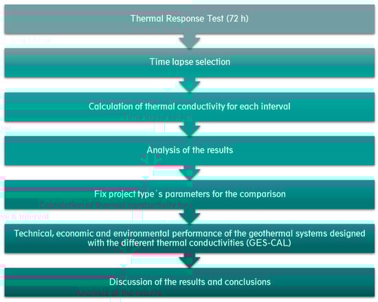
Figure 1.
Workflow scheme of the present research.
The geothermal pilot project has been dimensioned, according to the average thermal needs for domestic uses in Europe [31,32]. This will allow a comparison among the different bore fields obtained for each time lapse of the thermal test.
As shown in Figure 1, the software GES-CAL [33] is used in the final stage of the research. This software is capable of designing low-enthalpy geothermal systems and offers an estimation of the technical, economic, and environmental behavior of them. The final step of the workflow “Discussion of the results and conclusions” is based on the thermal conductivity results previously calculated. However, all the technical, environmental, and economic analysis is also included to highlight the previous assertions.
With all the information gathered, this project wishes to give some insight into the convenience of extending the TRT longer than is used nowadays.
2. Materials and Methods
2.1. Borehole under Study
The thermal response test included in the present work has been performed in a borehole located in the center of Spain (Ávila). The geological composition of the area is mainly defined by igneous and metamorphic formations and by principally sedimentary materials belonging to the Mesozoic, Tertiary, and Quaternary. An accurate geological characterization of the ground derived from geophysical prospecting in the borehole location can be consulted in a previous author’s works [34]. It must be mentioned that as stated in previous works [8], the complexity level of this environment (at shallow depths) constitutes an appropriate location for the analysis of the results of this study.
Regarding the construction of the geothermal borehole, it is constituted by a single-U polyethylene heat exchanger of 32 mm of diameter with several spacers along the tube. The stratigraphic column of the well brought to light the presence of water in almost the whole length. Thus, the grouting material was in this case the existing underground water. Inlet and outlet heat exchangers and the TRT device were connected by using externally insulated polyethylene tubes. The heat carrier fluid was water at a temperature of 10 °C, approximately. In Table 1 it is possible to observe the details of the entire borehole system.

Table 1.
Characteristics of the borehole system.
2.2. TRT Device
The TRT equipment used in this research and supplied by the Spanish company INGEO, is designed to work in double-U and single-U tube modes. As the standard TRT apparatus, it is constituted by a circulating pump that maintains the flow rate constant during the whole test and an electric heating device that heats the liquid of the circuit. The heating system is constituted by a resistance that enables working in three different heating levels (3 kW, 6 kW, and 9 kW). The data acquisition system includes the Kamstrup Multical-801 logger, commonly used for the measurement of parameters under temperature ranges of 2–180 °C [34,35]. Thanks to this device, the inlet and outlet temperatures of the working fluid are recorded at different regular time intervals. Figure 2 shows a schema of the in situ test in the borehole considered here.
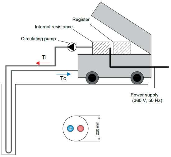
Figure 2.
Schema of the TRT device in the borehole under study.
2.3. Evaluation of the Test Results
There are currently multiple methods to evaluate the information obtained from the thermal response test, but the simplest way is the implementation of the line source theory (which is used here since the convective heat transfer is considered to be at negligible level). This model has been used since 1905 to determine the temperature distribution in the ground over time for geothermal ground source heat pump systems [36,37]. Considering the conditions of the borehole under study and given that, as mentioned above, the convective activity is almost imperceptible, the Infinite Line Source theory is appropriate for the resolution of the present approach. Following the approximation of Eklöf and Gehlin, the following Equation (1) is commonly applied to obtain the thermal conductivity of the ground from the TRT data [38,39].
where:
- Q = heat injection/extraction (W)
- = inclination of the temperature curve versus logarithmic time
- H = borehole heat exchanger depth (m)
- k = effective thermal conductivity of the ground (W/mK)
To finally calculate the thermal conductivity of the ground, Equation (1) must be transformed into Equation (2).
The duration of the global TRT is defined by the number of early data that should be discarded to obtain the ground thermal conductivity (commonly the first 10 h) according to the interpretation of the above mentioned line source method [39]. Based on the international standards, the minimum duration usually established for a TRT of a borehole heat exchanger is of around 48 h [40].
2.4. Testing Procedure
TRT was performed at the experimental well in the period of 8–11 June 2020. In this way, the global duration of the test was 72 h working in the first heating stage corresponding to 3 kW. From the entire TRT, different time intervals were selected for the calculation of the effective ground thermal conductivity. The first interval was established according to the Spanish Regulation UNE-EN ISO 17628, which establishes the minimum duration of the test by applying Equation (3) [41]. This regulation considers a range of thermal conductivities of the most common geothermal grouts, in which is included the one of the work.
where:
- r = radius of the borehole (m)
- ke = preliminary thermal conductivity (W/mK)
- cv = volumetric thermal capacity (J/m3/K)
Based on the lithological column, the estimated thermal conductivity and the volumetric thermal capacity of the surrounding materials were defined as 1.80 W/mK and 2.16·106 J/m3/K, respectively [42]. By substituting the above values and the radius of the well, the minimum duration recommended for the implementation of the TRT is in this case of 20.25 h. This means that, according to the mentioned regulation, the duration of test in the conditions of this study must be of at least 20.25 h.
Once the first time lapse is established, the intervals included in Table 2 are also considered in the study. As can be observed in the mentioned Table 2, the last interval corresponds to the duration of the entire test. The third column of this table also presents the time step of the stationary regime selected for each of the intervals under study. The subsequent calculation of the effective thermal conductivity will be made on each of these selected time steps.
Table 2.
Duration of each test interval and stationary time steps.
It must be mentioned that the stationary time steps presented in the previous Table 2 have been obtained by observing the period of time of each interval in which inlet and outlet temperatures begin to behave in a more constant way and considering a representative time lapse. In this way, in order to consider a representative and long enough time step, the stationary step for interval 1 (the shortest test) starts before the one of interval 2 and so on. It is also convenient to clarify that, in the real practice of a TRT, the exact stationary regime is not achieved, since periods of more than 100 h (depending on the borehole) would be needed. Thus, an approximation to the stationary regime is usually assumed.
3. Results
3.1. Time Lapse Results
The results of the entire TRT are shown in Figure 3. From the global curves of inlet and outlet fluid temperatures, the curves associated with each of the intervals described in Table 2 are plotted in the following Figure 4, Figure 5, Figure 6, Figure 7, Figure 8 and Figure 9. These figures also present the section of the stationary regime selected (for one of the inlet–outlet curves) and the equation associated with the straight line of each graphic.
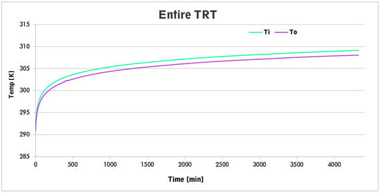
Figure 3.
Inlet and outlet fluid temperatures (entire TRT, 72 h).
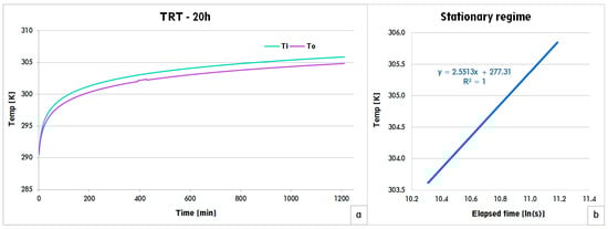
Figure 4.
(a) TRT results for the time lapse of 20 h, (b) stationary regime considering 700 sampling values.
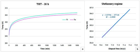
Figure 5.
(a) TRT results for the time lapse of 30 h, (b) stationary regime considering 1100 sampling values.
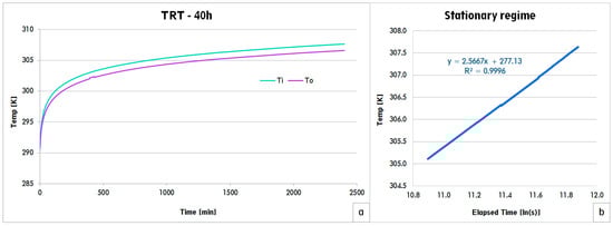
Figure 6.
(a) TRT results for the time lapse of 40 h, (b) stationary regime considering 1500 sampling values.
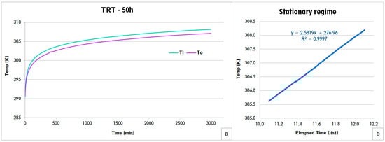
Figure 7.
(a) TRT results for the time lapse of 50 h, (b) stationary regime considering 1900 sampling values.
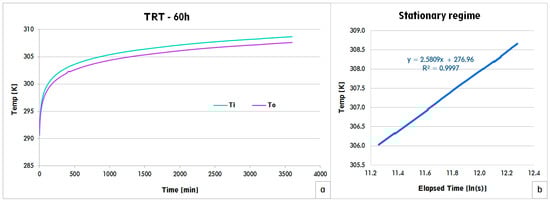
Figure 8.
(a) TRT results for the time lapse of 60 h, (b) stationary regime considering 2300 sampling values.
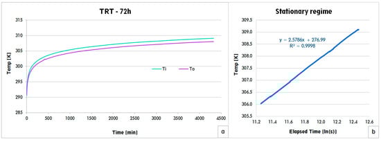
Figure 9.
(a) TRT results for the time lapse of 72 h, (b) stationary regime considering 2825 sampling values.
As can be seen above, Figure 3, in which the global thermal response test is included, shows the evolution of the inlet and outlet temperatures from the transitory to the stationary regime. In the remaining Figure 4, Figure 5, Figure 6, Figure 7, Figure 8 and Figure 9, it is possible to observe the evolution of the TRT until the period of each of them and the section of the test considered as stationary, for which the equation of the line and the correlation coefficient (R) are presented.
3.2. Ground Thermal Conductivity
From the results of Section 3.1, and using Equation (2), thermal conductivities for all the elapsed times considered have been calculated. Table 3 shows the results.
Table 3.
Calculation of the effective thermal conductivities for each time interval.
All these thermal conductivities will be included in the design process of the geothermal systems of the following Section 3.3.
3.3. Geothermal System Design
With the aim of evaluating how the variation of the thermal conductivity of the ground affects the general geothermal bore field, this subsection addresses the design of the system by the use of the specific geothermal software GES-CAL.
3.3.1. Initial Conditions
As stated in the introduction, a domestic pilot geothermal system has been established in order to observe the difference in the designing results due to the different thermal conductivities obtained in Section 3.2. In previous works [32], different thermal needs for different European thermal regions were defined. Our pilot system was located in the Spanish province of Ávila, in a granite-based geological environment, and a thermal demand per year of 40 MWh was selected according to the previously cited paper. The location of the shallow geothermal system also corresponds to the location of the borehole where the thermal response test has been performed. Figure 10 shows a capture of the geological map of the area in which some details about the location and the geological environment [43] of the project’s area can be observed.
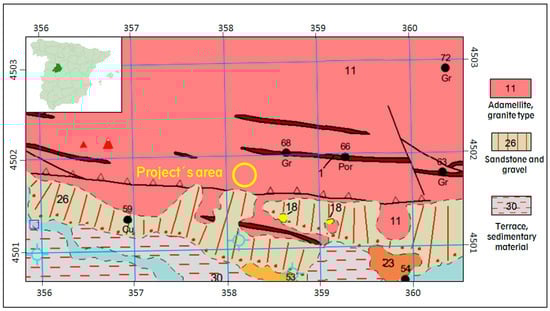
Figure 10.
Location and geological information of the borehole and geothermal system, UTM coordinates (103).
Figure 11 presents the monthly distribution considered of the aforementioned thermal needs, in order to make reproducible the designing process of the well field for each thermal conductivity value.
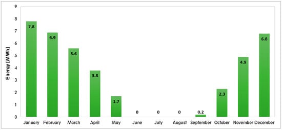
Figure 11.
Monthly distribution of the thermal energy needs in the geothermal project.
The months with the highest energy demand will be used to establish the power needs of the geothermal heat pump taking into account the estimated hours of operation and the coefficient of performance (COP) of the device.
3.3.2. Software GES-CAL
GES-CAL software has been recently developed by members from the TIDOP Research Group (belonging to the University of Salamanca) for the technical design of shallow closed-loop geothermal energy systems [33]. Unlike other existing tools, GES-CAL enables defining all the most common heat exchanger configurations (vertical double-U and single-U, horizontal and helical ones). By only introducing initial information about the area where the systems will be installed and specific geothermal parameters (heat pump, heat exchanger configuration, grouting material, etc.), GES-CAL automatically provides several options about the technical design of the shallow system in addition to an environmental and economic analysis of the selected solution. In a summarized way, the steps to be followed in the tool are:
- Energy demandIf known, the user can directly introduce the heating/cooling energy demand. Additionally, GES-CAL is constituted by a specific module that allows the calculation of this value from some previously inserted information about the space. In the case of this work, as stated in the previous subsection, the heating energy demand of the system under study has already been established.
- Heat pumpThe user is required to specify the operating mode of the heat pump, the annual operative period, and its initial COP. From these data, GES-CAL defines the final power of the heat pump included in the system. In the installation here analyzed, the operative period will be 2400 h/year and an initial heat pump COP of 4 will be considered.
- GroundIn this step, the user must introduce the available area of the surrounding ground (length and width) and its thermal conductivity. In this sense, if the system is planned in the Spanish province of Ávila, the software is capable of automatically obtaining the specific ground thermal conductivity by clicking on the particular area of the map that the tool provides. In this work, the ground thermal conductivity will be manually introduced based on the values calculated in Table 3.
- Geothermal configurationAs already mentioned, one of main strengths of GES-CAL is the possibility of calculating the systems with different heat exchanger designs. In this stage, the user must select the configuration of the heat exchangers that better meet the project requirements. For the system here considered, all the solutions will be studied with the principal aim of evaluating the variation of the ground thermal conductivity in each design. It is important to clarify that, although the TRT has been made on a borehole with single-U heat exchangers, the final configuration of the geothermal system will depend on the final results of GES-CAL, which will define the most suitable solution.
- Technical designOnce all the above information is defined, GES-CAL software provides the technical scheme of the system in function of the previously selected heat exchanger configuration. The user is here capable of choosing one of the options proposed by the tool.
- Economic and environmental evaluationThese two modules offer the possibility of: (i) determining the initial investment required and the costs associated with the designed geothermal system and comparing it to the most frequent energy sources and (ii) calculating the greenhouse gas emissions derived from the system operation and establishing the same energy comparison.
The following Table 4 summarizes the input data of the geothermal system considered in this work.
Table 4.
Input data of the geothermal systems to be introduced in GES-CAL software.
From the data presented in the previous Table 4, the results of applying GES-CAL software to each TRT time interval are shown in the following Table 5, Table 6, Table 7, Table 8, Table 9 and Table 10.
Table 5.
Design provided by GES-CAL software for the geothermal system under study, interval 1.
Table 6.
Design provided by GES-CAL software for the geothermal system under study, interval 2.
Table 7.
Design provided by GES-CAL software for the geothermal system under study, interval 3.
Table 8.
Design provided by GES-CAL software for the geothermal system under study, interval 4.
Table 9.
Design provided by GES-CAL software for the geothermal system under study, interval 5.
Table 10.
Design provided by GES-CAL software for the geothermal system under study, interval 6.
4. Discussion
4.1. Thermal Conductivity on the Different Time Lapses
The estimation of the loss of precision in thermal response tests of the ground due to the shortening of the measurement intervals has been carried out previously in some studies [44], all of them with different grouting materials for the boreholes, none of them with water as in this case. In the previously cited work, a study of this type was carried out on 15 different soundings, with a depth of around 60 m (similar to our case). In order to compare results, we have chosen the most similar borehole to ours among those of that study in terms of thermal conductivity values obtained. Since the measurement time intervals were not exactly the same as in this work, Table 11 is attached with the data from both essays for comparison.
Table 11.
Comparison of the thermal conductivity results of a water-filled well (this work) and a grouted one.
Additionally, Figure 12 shows the graphical evolution of the results obtained in both cases from Table 11.
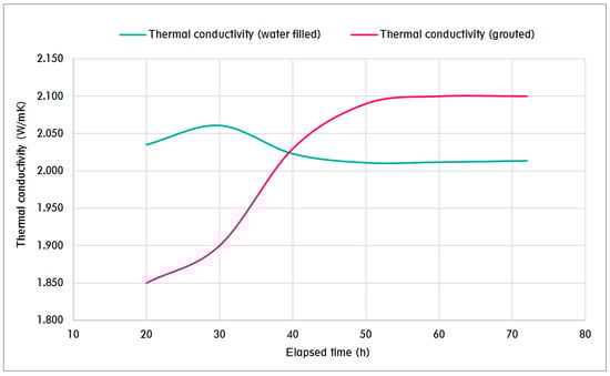
Figure 12.
Comparison between thermal conductivity evolutions.
The calculus for the six different time lapses established in this work shows very little variation in the results when using water as borehole filling material. The initial variation in slope (30 and 40 h) can be attributed to the data-collecting phase and the development of the experiment (inaccuracies have been described in the thermal response tests due to factors such as the instability of the electricity supply for the resistance in charge of heat input [45,46]). Thermal conductivity evolution from the grouted borehole test is much more pronounced, with variations of up to 10% versus 2.5% in water-filled.
Although in many engineering projects, 10% of uncertainty is acceptable in the input data of the design process and can be managed, results seem to show that water-filled boreholes behave in a more consistent way in terms of reducing the duration of the thermal response tests. The grouted borehole [40] considered here is drilled in a less homogeneous geological environment (Quaternary and Miocene materials in layers) than our granite area. This could be also a source for the more pronounced sensibility to the length of the measurement process.
It must be also mentioned that the assumption considered here (time lapses from 20 to 72 h) is acceptable because times are higher than the thermal instability of the ground for 1–3 boreholes (the ones obtained in the geothermal design). However, if a higher number of pipes was used, longer times should be included in the analysis [47,48].
4.2. Influence on the Geothermal Design
The final objective of the research here included is to analyze if the differences in the results of the ground thermal conductivity associated with each time interval are significant in the global design of the system. Thus, based on the results of the previous Table 5, Table 6, Table 7, Table 8, Table 9 and Table 10, it is possible to observe in Figure 13 the total drilling length and pipe length (in the case of the horizontal design) required in each interval for each configuration of heat exchanger.
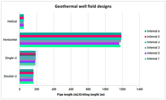
Figure 13.
Bore field design required in each interval as a function of the heat exchanger configuration.
In the graphic of the above Figure 13, it is quite noticeable that the differences among the intervals in each configuration are practically nonexistent. It must be also mentioned from the results of GES-CAL that the operational costs are identical in all designs and time intervals. This fact is because these costs mainly derive from the heat pump electricity use, its power being the same for all the options considered (the heating energy demand is identical for all of them). In the same way, CO2 emissions are also the same for all cases because of the identical heat pump electricity use.
Analyzing now in Figure 14 the initial investment required by the systems of each interval, as happened in Figure 13, results are practically the same among intervals within the same group of heat exchangers.
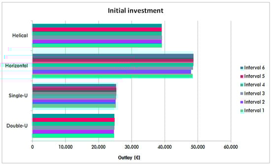
Figure 14.
Initial investment associated with each interval as a function of the heat exchanger configuration.
From all the above, it can be preliminary deduced that, in the case of the installation considered in this research, the differences among the thermal conductivity results obtained in different time intervals of the TRT are not significant in the subsequent well field design.
Focusing now on the most optimal configuration for the geothermal system of this research (the vertical double-U), as already mentioned, the total drilling length is similar for all the intervals and therefore, the initial investments are also almost identical. For a deeper analysis, it is convenient to consider the price of the realization of a thermal response test in the area of the study. According to the Spanish company CYPE Ingenieros S.A., the cost of a conventional TRT of 48 h is around 4000 €. As can be seen in Table 12, more than a half of this value corresponds to variable costs that are directly related to the duration of the test. These variable costs mainly refers to the operating time required by the technician in the development of the tests, that is to say, the period of measuring time and the amount of data to be processed (proportional to the duration of the TRT).
Table 12.
Cost of performing a TRT in Spain.
Considering the information of Table 12, the price of the TRTs for the time intervals included in this research has been estimated as Table 13 shows.
Table 13.
Estimation of the cost of the TRTs for the time intervals considered in this work.
The data of Table 13 clearly show significant differences in the price of the TRT as a function of its duration. According to the results of this research, the thermal conductivities obtained in the six time lapses are almost identical, meaning that for the characteristics of the borehole under study, performing a TRT of 20 h provides similar results to one of 72 h, achieving an important reduction in the cost of the test (more than half).
5. Conclusions
This paper presents the results obtained from a thermal response test of a water-filled borehole performed in the province of Ávila, Spain. From the global test of 72 h, different shorter time intervals have been considered, calculating the ground thermal conductivity in each single lapse. Once this parameter was defined, GES-CAL software was used to design the closed-loop geothermal system with the different obtained thermal conductivity values. The results clearly show that there are no substantial differences among the thermal conductivities obtained in each time interval. Derived from this fact, the designs of the geothermal bore fields are consequently almost identical in all intervals for each of the heat exchanger configurations and hence, the initial investment of each system is also similar. Despite the fact that the principal objective of this work is to analyze the reduction in the data acquisition time of the TRT, the GES-CAL tool is required to identify the influence of the thermal conductivity results on the final bore field design.
Additionally, the analysis of the price of carrying out a TRT in the area of the study has revealed the high increment of this price when the duration of the test increases from 20 h to 72 h.
In summary, the principal statements deduced from the results of this research are:
- In the borehole of the study, the thermal conductivity of the ground calculated from the TRT did not present substantial variations when using different test durations. This may be due to the fact that the borehole was water-filled instead of being grouted (as usual). Also, the homogeneous geological environment (granite) of the area may have had some influence on this result (Figure 12).
- The geothermal designs performed by GES-CAL software for all the ground thermal conductivities showed very little differences among them (when comparing the same type of geothermal system, as can be seen in Figure 13). This fact implies that all the designs demand similar initial investments for the same kind of ground heat exchanger considered.
- The cost of a TRT is highly influenced by the global test duration. In the borehole here considered, the reduction of the duration to 20 h means substantial savings in the final price of the TRT without resulting in high differences of the ground thermal conductivity.
- In small, shallow geothermal installations, as the one in this research, reducing the duration of the TRT could make it affordable in this kind of system where the budget is not extremely high.
Finally, it is important to clarify two main aspects about the applicability of the present research. The results of this work can be extended to those cases with similar test conditions, that is to say, water-filled boreholes located in granitic geological formations. Furthermore, it must be mentioned that in the case of geothermal installations planned to work only in heating mode, the thermal conductivity, temperature, and moisture of the ground could change over time (after 3–4 years of operation). In this sense, future studies will be directed at the analysis of thermal response tests in different sites and geothermal configurations as well as the evaluation of the variation of the thermal behavior of the system over time.
Author Contributions
Conceptualization, C.S.B. and I.M.N.; methodology, C.S.B. and I.M.N.; software, C.S.B. and I.M.N.; validation, A.F.M., and D.G.-A.; formal analysis, A.F.M., and D.G.-A.; investigation, C.S.B. and I.M.N.; resources, C.S.B. and I.M.N.; data curation, A.F.M., and D.G.-A.; writing—original draft preparation, C.S.B. and I.M.N.; writing—review and editing, C.S.B., I.M.N., A.F.M., and D.G.-A.; supervision, A.F.M., and D.G.-A. All authors have read and agreed to the published version of the manuscript.
Funding
This research received no external funding.
Acknowledgments
Authors want to thank the Department of Cartographic and Terrain Engineering of the Higher Polytechnic School of Avila, University of Salamanca, for allowing the use of all the laboratories and devices that have been essential for the realization of the experimental stages included in this work. Authors would also like to thank the University of Salamanca and Santander Bank for the pre-doctoral Grant (Program III USAL Grant) provided to the corresponding author of this paper.
Conflicts of Interest
The authors declare no conflict of interest.
References
- Yildirim, N.; Toksoy, M.; Gokcen, G. Piping network design of geothermal district heating systems: Case study for a university campus. Energy 2010, 35, 3256–3262. [Google Scholar] [CrossRef]
- Marcotte, D.; Pasquier, P.; Sheriff, F.; Bernier, M. The importance of axial effects for borehole design of geothermal heat-pump systems. Renew. Energy 2010, 35, 763–770. [Google Scholar] [CrossRef]
- Blázquez, C.S.; Verda, V.; Nieto, I.M.; Martín, A.F.; González-Aguilera, D. Analysis and optimization of the design parameters of a district groundwater heat pump system in Turin, Italy. Renew. Energy 2020, 149, 374–383. [Google Scholar] [CrossRef]
- Sáez Blázquez, C.; Farfán Martín, A.; Nieto, I.M.; González-Aguilera, D. Economic and environmental analysis of different district heating systems aided by geothermal energy. Energies 2018, 11, 1265. [Google Scholar] [CrossRef]
- UNE-EN 16147:2017. Heat pumps with electrically driven compressors—Testing, performance rating and requirements for marking of domestic hot water units. Asociación Española de Normalización y Certificación 2017. [Google Scholar]
- Blázquez, C.S.; Martín, A.F.; Nieto, I.M.; García, P.C.; Pérez, L.S.S.; Aguilera, D.G. Thermal conductivity map of the Avila region (Spain) based on thermal conductivity measurements of different rock and soil samples. Geothermics 2017, 65, 60–71. [Google Scholar] [CrossRef]
- Sáez Blázquez, C.; Farfán Martín, A.; Martín Nieto, I.; González-Aguilera, D. Measuring of thermal conductivities of soils and rocks to be used in the calculation of a geothermal installation. Energies 2017, 10, 795. [Google Scholar] [CrossRef]
- Nieto, I.M.; Martín, A.F.; Blázquez, C.S.; Aguilera, D.G.; García, P.C.; Vasco, E.F.; García, J.C. Use of 3D electrical resistivity tomography to improve the design of low enthalpy geothermal systems. Geothermics 2019, 79, 1–13. [Google Scholar] [CrossRef]
- Yu, M.Z.; Peng, X.F.; Li, X.D.; Fang, Z.H. A simplified model for measuring thermal properties of deep ground soil. Exp. Heat Transf. 2004, 17, 119–130. [Google Scholar] [CrossRef]
- Kavanaugh, S.P. Field tests for ground thermal properties—Methods and impact on ground-source heat pump design. Univ. Ala. Tuscaloosa 2000, 119, 109575. [Google Scholar]
- Wilke, S.; Menberg, K.; Steger, H.; Blum, P. Advanced thermal response tests: A review. Renew. Sustain. Energy Rev. 2020, 119, 109575. [Google Scholar] [CrossRef]
- Antelmi, M.; Alberti, L.; Angelotti, A.; Curnis, S.; Zille, A.; Colombo, L. Thermal and hydrogeological aquifers characterization by coupling depth-resolved thermal response test with moving line source analysis. Energy Convers. Manag. 2020, 225, 113400. [Google Scholar] [CrossRef]
- Fossa, M.; Minchio, F.; Rolando, D. Thermal Response Test experiments and modelling applied to shallow geothermal piles of different geometry. SHAREOK 2018. [Google Scholar] [CrossRef]
- McDaniel, A.; Tinjum, J.; Hart, D.J.; Lin, Y.F.; Stumpf, A.; Thomas, L. Distributed thermal response test to analyze thermal properties in heterogeneous lithology. Geothermics 2018, 76, 116–124. [Google Scholar] [CrossRef]
- Jensen-Page, L.C. Measurement of Ground Thermal Properties for Shallow Geothermal Applications. Ph.D. Thesis, University of Melbourne, Melbourne, Australia, 2019. [Google Scholar]
- Li, M.; Zhang, L.; Liu, G. Estimation of thermal properties of soil and backfilling material from thermal response tests (TRTs) for exploiting shallow geothermal energy: Sensitivity, identifiability, and uncertainty. Renew. Energy 2019, 132, 1263–1270. [Google Scholar] [CrossRef]
- Verdecchia, A.; Brunelli, D.; Tinti, F.; Barbaresi, A.; Tassinari, P.; Benini, L. Low-cost micro-thermal response test system for characterizing very shallow geothermal energy. In Proceedings of the 2016 IEEE Workshop on Environmental, Energy, and Structural Monitoring Systems (EESMS), Bari, Italy, 13–14 June 2016; pp. 1–6. [Google Scholar]
- Raymond, J.; Malo, M.; Lamarche, L.; Perozzi, L.; Gloaguen, E.; Bégin, C. New methods to spatially extend thermal response test assessments. SHAREOK 2017. [Google Scholar] [CrossRef]
- Yang, X.; Wei, P.; Cui, X.; Jin, L.; He, Y.L. Thermal response of annuli filled with metal foam for thermal energy storage: An experimental study. Appl. Energy 2019, 250, 1457–1467. [Google Scholar] [CrossRef]
- Choi, W.; Ooka, R. Effect of natural convection on thermal response test conducted in saturated porous formation: Comparison of gravel-backfilled and cement-grouted borehole heat exchangers. Renew. Energy 2016, 96, 891–903. [Google Scholar] [CrossRef]
- Sliwa, T.; Rosen, M.A. Efficiency analysis of borehole heat exchangers as grout varies via thermal response test simulations. Geothermics 2017, 69, 132–138. [Google Scholar] [CrossRef]
- Minchio, F.; Cesari, G.; Pastore, C.; Fossa, M. Experimental Hydration Temperature Increase in Borehole Heat Exchangers during Thermal Response Tests for Geothermal Heat Pump Design. Energies 2020, 13, 3461. [Google Scholar] [CrossRef]
- ISO 17628:2015. Geotechnical Investigation and Testing—Geothermal Testing—Determination of Thermal Conductivity of Soil and Rock Using a Borehole Heat Exchanger; CEN: Brussels, Belgium, 2015. [Google Scholar]
- Blázquez, C.S.; Martín, A.F.; Nieto, I.M.; García, P.C.; Pérez, L.S.S.; González-Aguilera, D. Analysis and study of different grouting materials in vertical geothermal closed-loop systems. Renew. Energy 2017, 114, 1189–1200. [Google Scholar] [CrossRef]
- Spitler, J.D.; Javed, S.; Ramstad, R.K. Natural convection in groundwater-filled boreholes used as ground heat exchangers. Appl. Energy 2016, 164, 352–365. [Google Scholar] [CrossRef]
- Johnsson, J.; Adl-Zarrabi, B. Modelling and evaluation of groundwater filled boreholes subjected to natural convection. Appl. Energy 2019, 253, 113555. [Google Scholar] [CrossRef]
- Javed, S.; Spitler, J.D. Calculation of borehole thermal resistance. In Advances in Ground-Source Heat Pump Systems; Cambridge International Science; Woodhead Publishing: Cambridge, UK, 2016; pp. 63–95. [Google Scholar]
- Erol, S.; François, B. Efficiency of various grouting materials for borehole heat exchangers. Appl. Therm. Eng. 2014, 70, 788–799. [Google Scholar] [CrossRef]
- Indacoechea-Vega, I.; Pascual-Muñoz, P.; Castro-Fresno, D.; Calzada-Pérez, M.A. Experimental characterization and performance evaluation of geothermal grouting materials subjected to heating–cooling cycles. Constr. Build. Mater. 2015, 98, 583–592. [Google Scholar] [CrossRef]
- Pascual-Muñoz, P.; Indacoechea-Vega, I.; Zamora-Barraza, D.; Castro-Fresno, D. Experimental analysis of enhanced cement-sand-based geothermal grouting materials. Constr. Build. Mater. 2018, 185, 481–488. [Google Scholar] [CrossRef]
- Nieto, I.M.; Borge-Diez, D.; Sáez Blázquez, C.; Martín, A.F.; González-Aguilera, D. Study on Geospatial Distribution of the Efficiency and Sustainability of Different Energy-Driven Heat Pumps Included in Low Enthalpy Geothermal Systems in Europe. Remote Sens. 2020, 12, 1093. [Google Scholar] [CrossRef]
- Blázquez, C.S.; Borge-Diez, D.; Nieto, I.M.; Martín, A.F.; González-Aguilera, D. Technical optimization of the energy supply in geothermal heat pumps. Geothermics 2019, 81, 133–142. [Google Scholar] [CrossRef]
- Blázquez, C.S.; Nieto, I.M.; Mora, R.; Martín, A.F.; González-Aguilera, D. GES-CAL: A new computer program for the design of closed-loop geothermal energy systems. Geothermics 2020, 87, 101852. [Google Scholar] [CrossRef]
- Sáez Blázquez, C.; Martín Nieto, I.; Farfán Martín, A.; González-Aguilera, D.; Carrasco García, P. Comparative Analysis of Different Methodologies Used to Estimate the Ground Thermal Conductivity in Low Enthalpy Geothermal Systems. Energies 2019, 12, 1672. [Google Scholar] [CrossRef]
- Alberdi-Pagola, M. Thermal response test data of five quadratic cross section precast pile heat exchangers. Data Brief 2018, 18, 13–15. [Google Scholar] [CrossRef] [PubMed]
- Ingersoll, L.R.; Plass, H.J. Theory of the ground pipe source for the heat pump. ASHRAE Trans. 1948, 54, 339–348. [Google Scholar]
- Jaeger, J.C.; Carslaw, H.S. Conduction of Heat in Solids; Oxford University Press: Oxford, UK, 1959. [Google Scholar]
- Eklöf, C.; Gehlin, S. TED. A Mobile Equipment for Thermal Response Test. Master’s Thesis, Luleå University of Technology, Luleå, Sweden, 1996. [Google Scholar]
- Sanner, B.; Hellström, G.; Spitler, J.; Gehlin, S. Thermal response test–current status and world-wide application. In Proceedings of the World Geothermal Congress, Antalya, Turkey, 24–29 April 2005; Volume 1436, p. 2005. [Google Scholar]
- Ashrae, T. Thermal Guidelines for Data Processing Environments-Expanded Data Center Classes and Usage Guidance; White Paper; ASHRAE: Atlanta, GA, USA, 2011. [Google Scholar]
- UNE-EN ISO 172628:2017. Geotechnical Investigation and Testing. Geothermal Testing. Determination of Thermal Conductivity of Soil and Rock Using a Borehole Heat Exchanger; International Organization for Standardization: Geneva, Switzerland, 2017. [Google Scholar]
- Prontuario de Soluciones Constructivas, Código Técnico de la Edificación (CTE); Instituto de Ciencias de la Construcción Eduardo Torroja e Instituto de la Construcción de Castilla y León: León, Spain, 2007.
- Magna 50, Mapa Geológico De España 1:50.000, HOJA 531, Ávila de los Caballeros; IGME, Instituto Geológico y Minero de España: Madrid, Spain, 2003.
- Bujok, P.; Grycz, D.; Klempa, M.; Kunz, A.; Porzer, M.; Pytlik, A.; Rozehnal, Z.; Vojčinák, P. Assessment of the influence of shortening the duration of TRT (thermal response test) on the precision of measured values. Energy 2014, 64, 120–129. [Google Scholar] [CrossRef]
- Beier, R.A. Deconvolution and convolution methods for thermal response tests on borehole heat exchangers. Geothermics 2020, 86, 101786. [Google Scholar] [CrossRef]
- Zhang, C.; Song, W.; Liu, Y.; Kong, X.; Wang, Q. Effect of vertical ground temperature distribution on parameter estimation of in-situ thermal response test with unstable heat rate. Renew. Energy 2019, 136, 264–274. [Google Scholar] [CrossRef]
- Hartley, J. Coupled heat and moisture transfer in soils: A review. Adv. Dry. 1987, 4, 199–248. [Google Scholar]
- Hartley, J.G.; Black, W.Z.; Bush, R.A.; Martin, M.A. Measurements, Correlations and Limitations of Soil Thermal Stability. Pergamon Press. 1982, 121–133. [Google Scholar]


Publisher’s Note: MDPI stays neutral with regard to jurisdictional claims in published maps and institutional affiliations. |
© 2020 by the authors. Licensee MDPI, Basel, Switzerland. This article is an open access article distributed under the terms and conditions of the Creative Commons Attribution (CC BY) license (http://creativecommons.org/licenses/by/4.0/).