Fluid–Structure Interaction Simulations of a Wind Gust Impacting on the Blades of a Large Horizontal Axis Wind Turbine


Abstract
:1. Introduction
2. Methodology
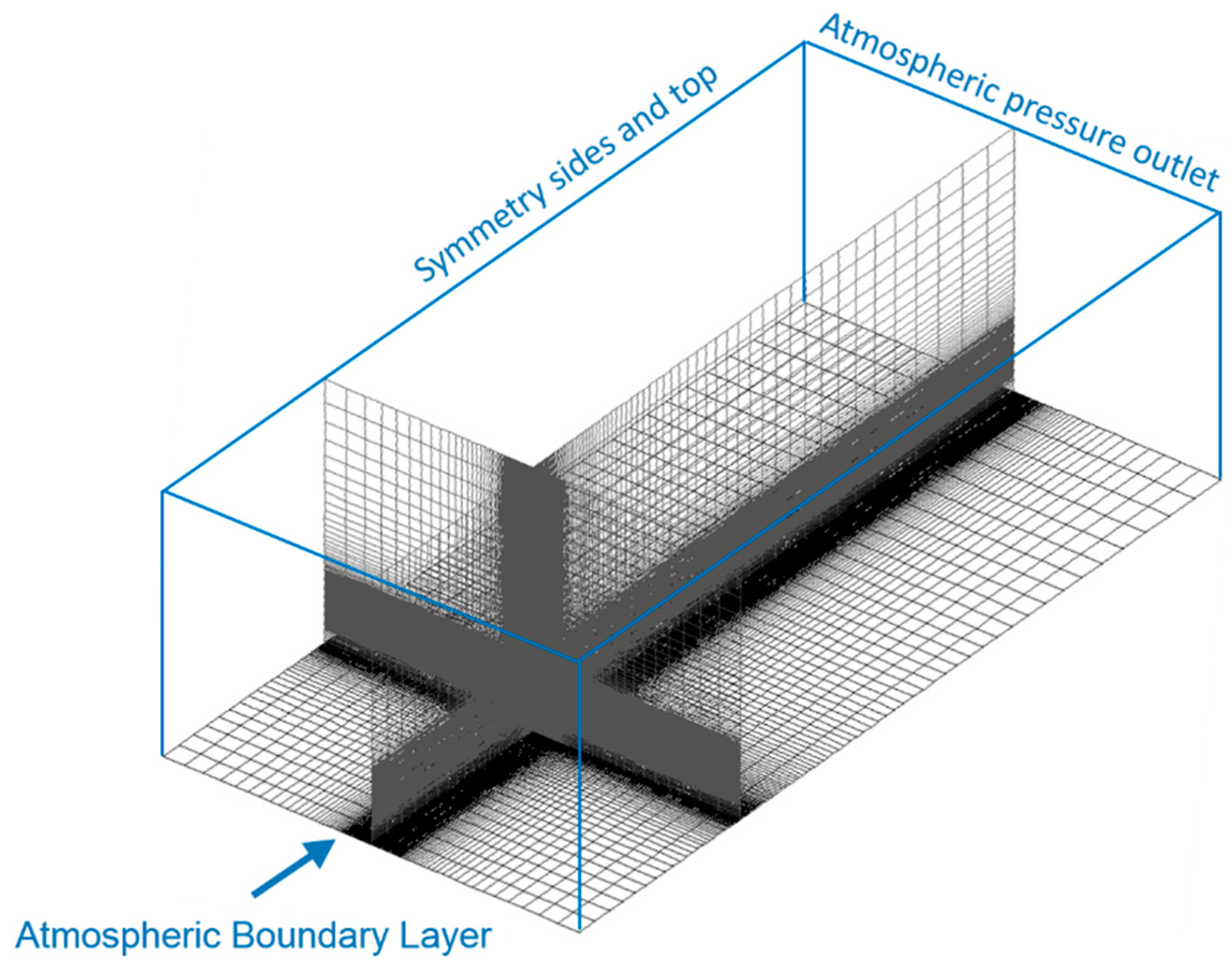
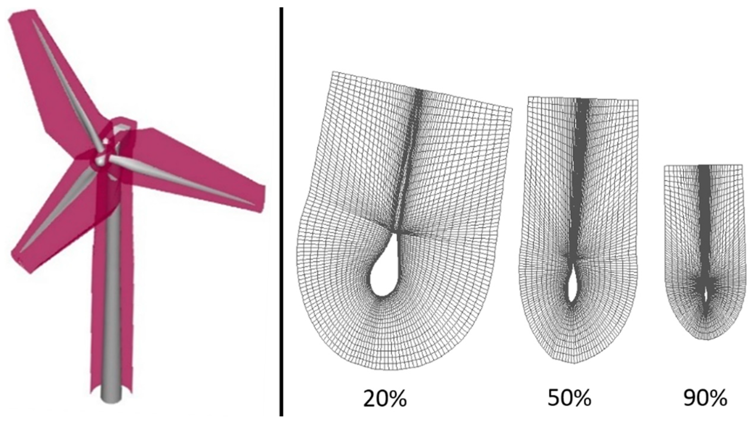
2.1. The CFD Model
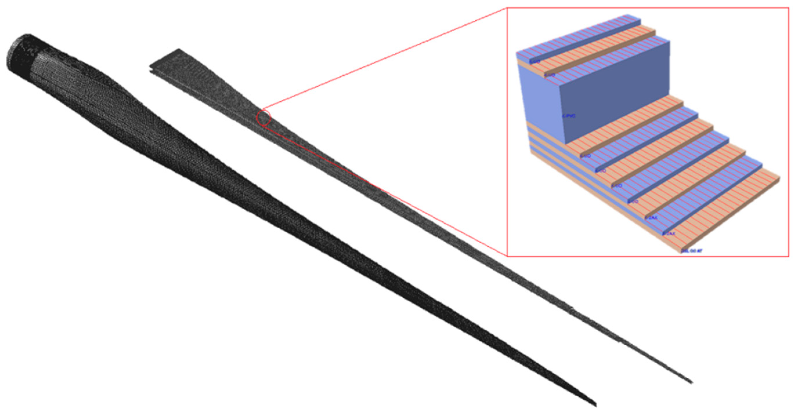
2.2. The Structural FEM Model
2.3. FSI Coupling
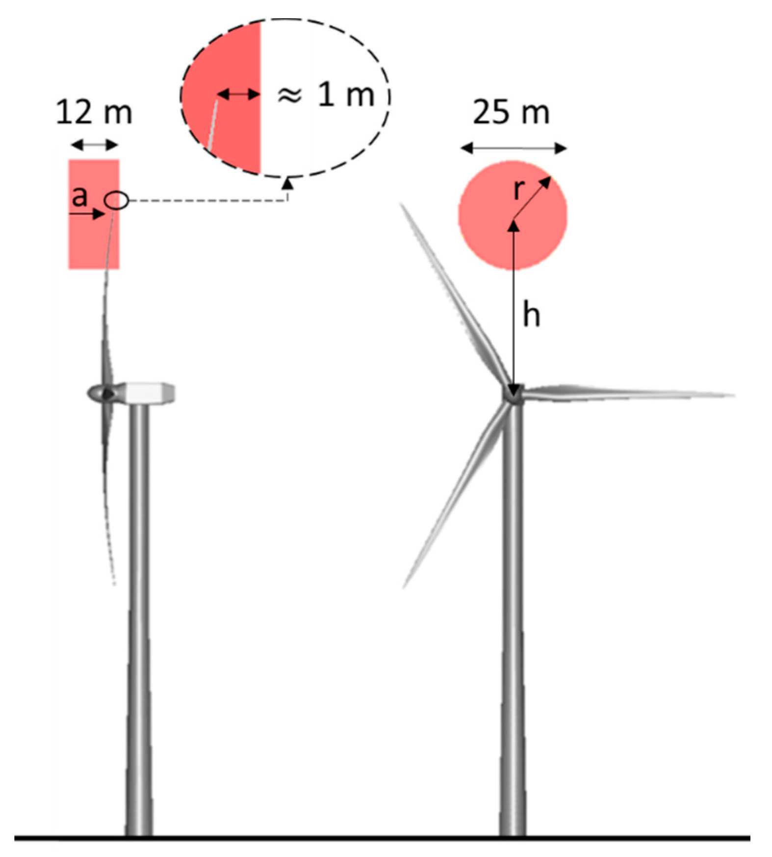
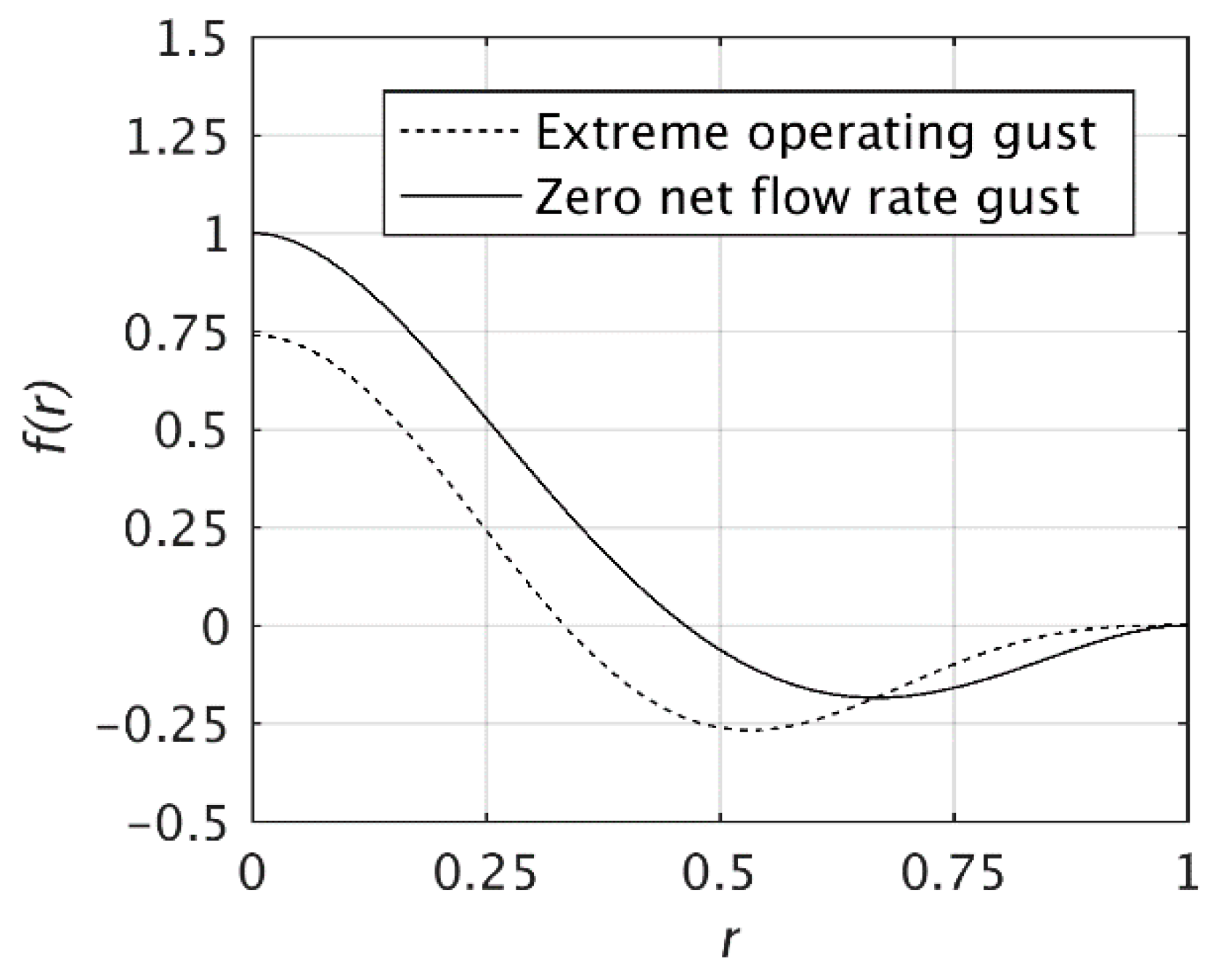
2.4. Gust Model
3. Results and Discussion
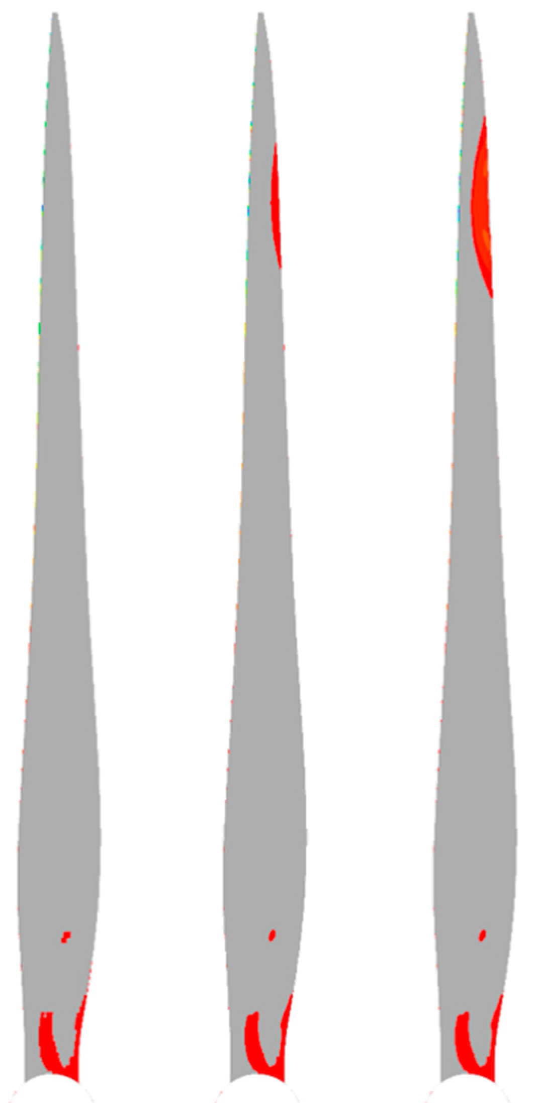
3.1. Zero Net Flow Rate Gust
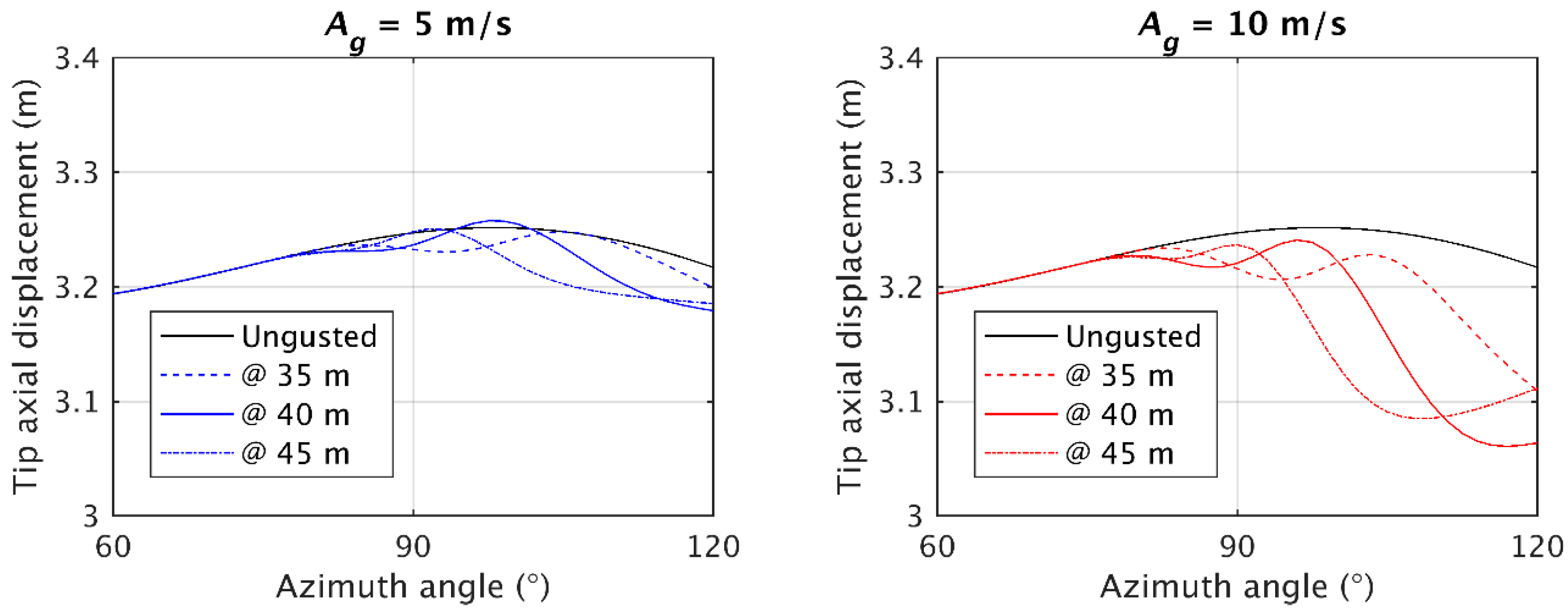
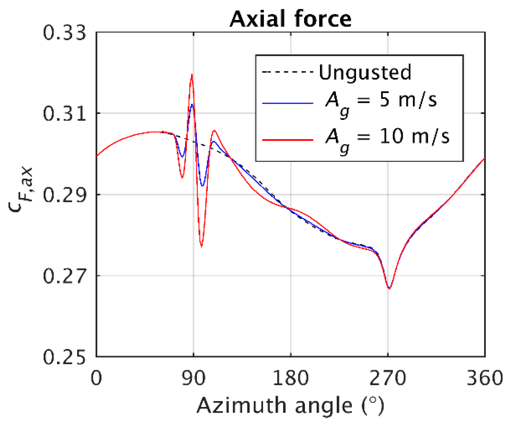
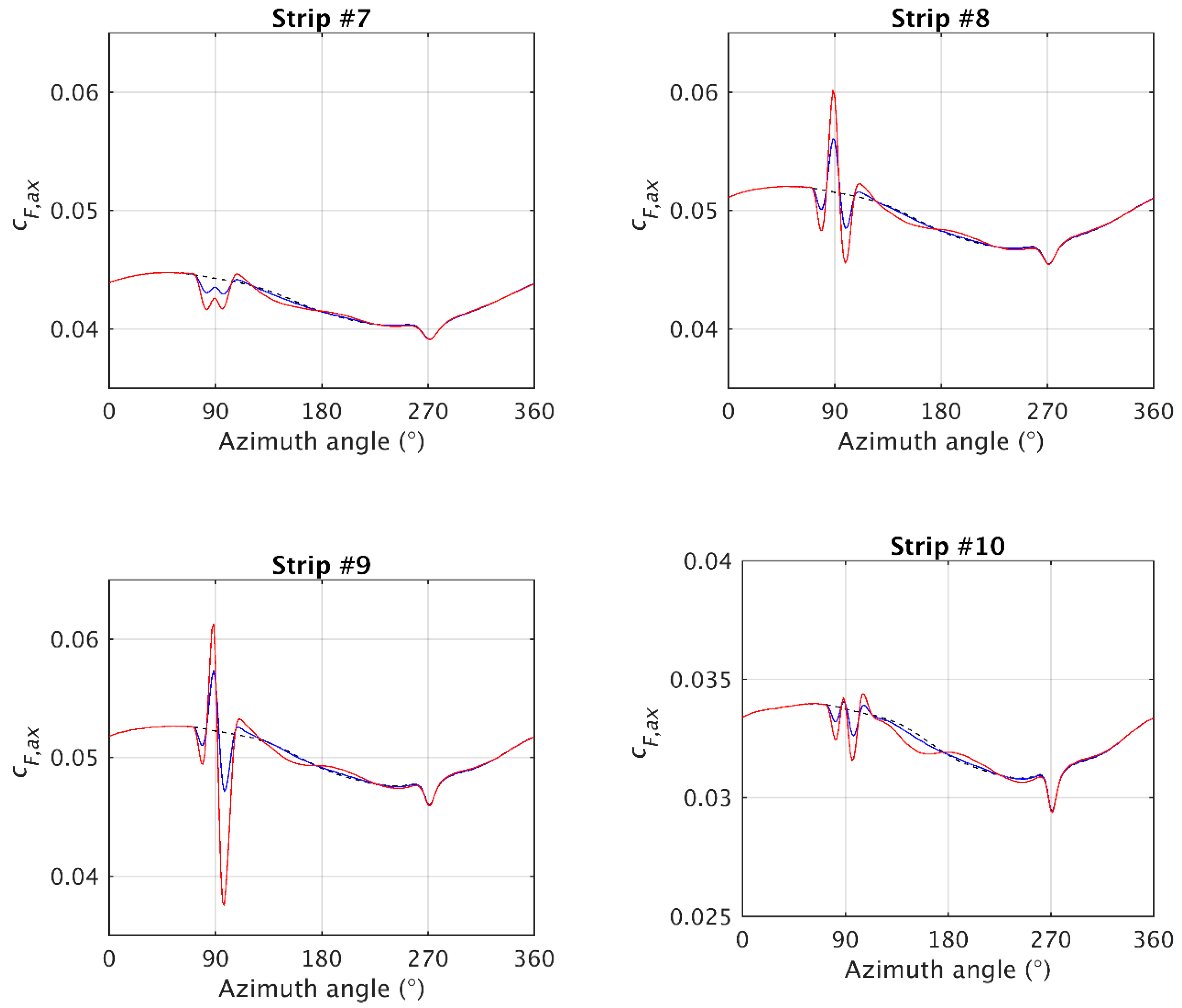
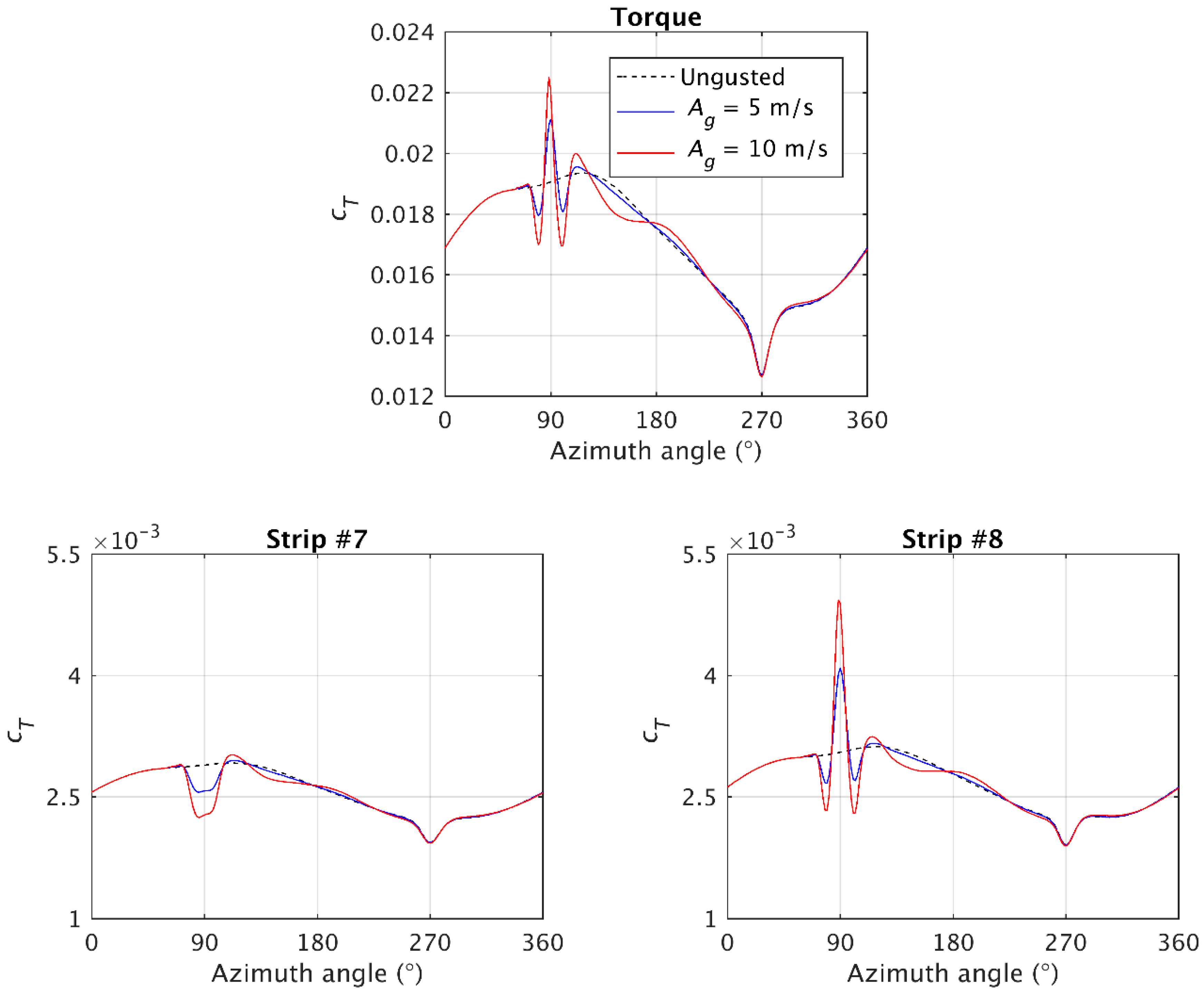
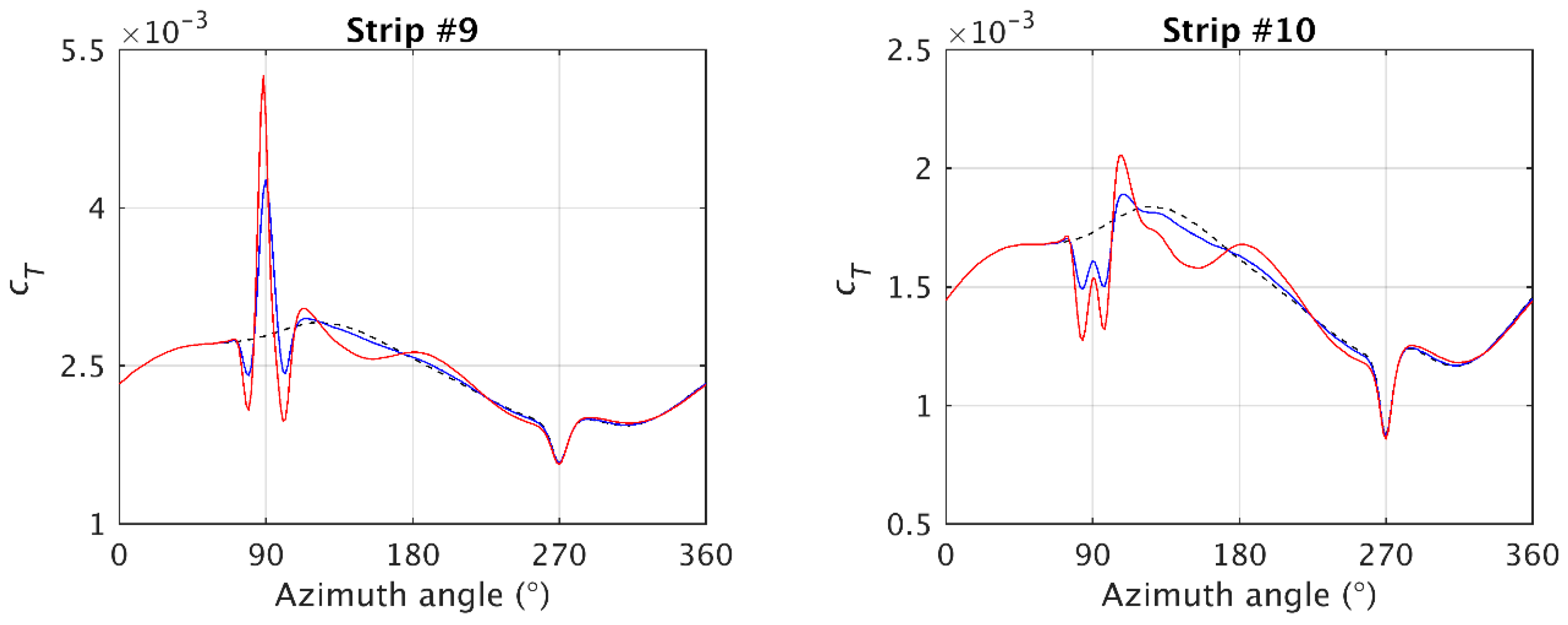
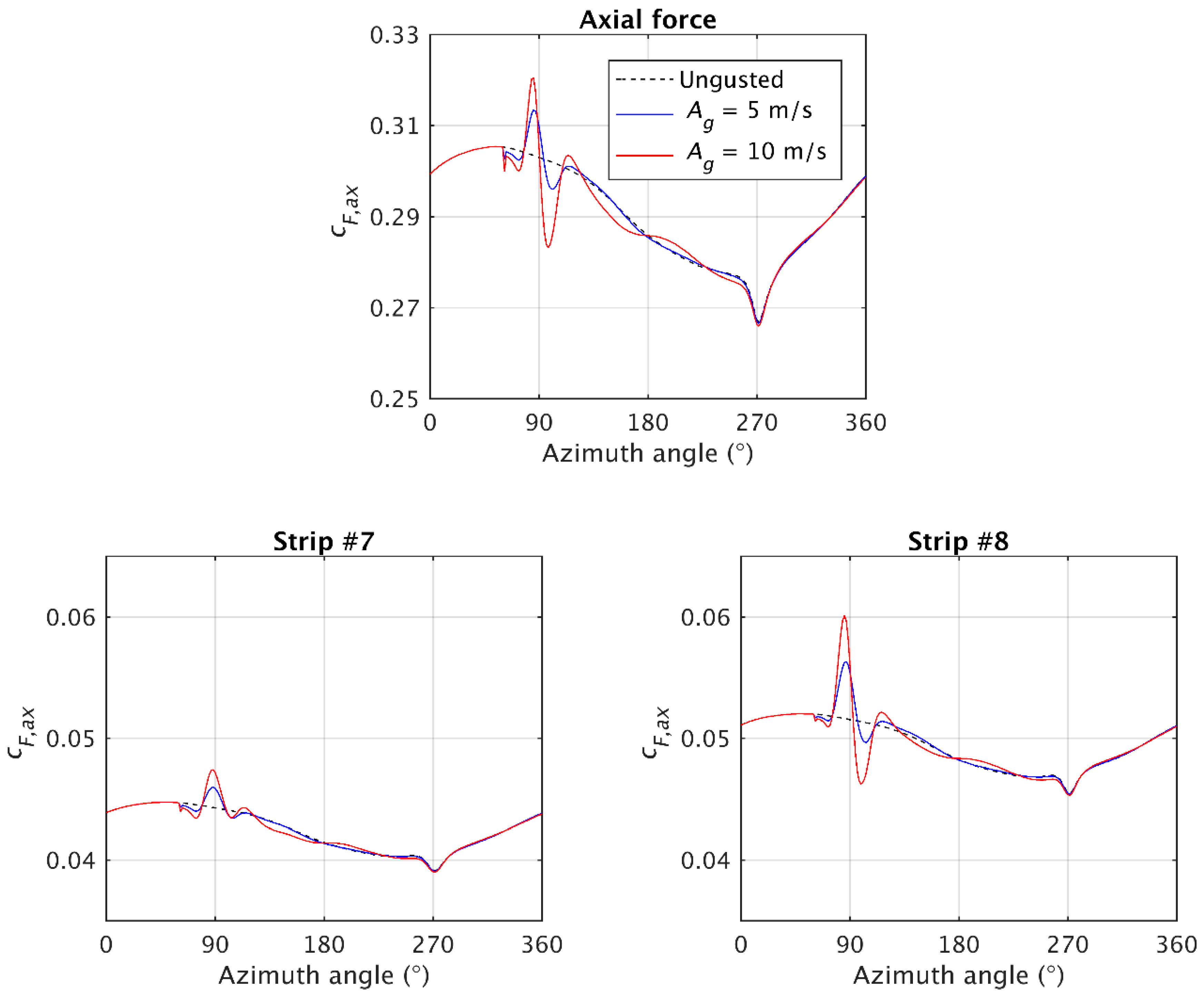
3.2. The 1 + Cos Gust
4. Conclusions
Author Contributions
Funding
Acknowledgments
Conflicts of Interest
References
- Caduff, M.; Huijbregts, M.A.J.; Althaus, H.J.; Koehler, A.; Hellweg, S. Wind power electricity: The bigger the turbine, the greener the electricity? Environ. Sci. Technol. 2012, 46, 4725–4733. [Google Scholar] [CrossRef]
- Bazilevs, Y.; Hsu, M.C.; Akkerman, I.; Wright, S.; Takizawa, K.; Henicke, B.; Spielman, T.; Tezduyar, T.E. 3D simulation of wind turbine rotors at full scale. Part I: Geometry modeling and aerodynamics. Int. J. Numer. Methods Fluids 2011, 65, 207–235. [Google Scholar] [CrossRef] [Green Version]
- Bazilevs, Y.; Hsu, M.C.; Akkerman, I.; Kiendl, J.; Wüchner, R.; Bletzinger, K.U. 3D simulation of wind turbine rotors at full scale. Part II: Fluid–structure interaction modeling with composite blades. Int. J. Numer. Methods Fluids 2011, 65, 236–253. [Google Scholar] [CrossRef]
- Hsu, M.C.; Bazilevs, Y. Fluid-structure interaction modelling of wind turbines: Simulating the full machine. Comput. Mech. 2012, 50, 821–833. [Google Scholar] [CrossRef]
- Liu, X.; Lu, C.; Liang, S.; Godbole, A.; Chen, Y. Vibration-induced aerodynamic loads on large horizontal axis wind turbine blades. Appl. Energy 2017, 185, 1109–1119. [Google Scholar] [CrossRef] [Green Version]
- Santo, G.; Peeters, M.; Van Paepegem, W.; Degroote, J. Dynamic load and stress analysis of a large Horizontal Axis Wind Turbine using full scale fluid-structure interaction simulation. Renew. Energy 2019, 140, 212–226. [Google Scholar] [CrossRef]
- Lee, Y.J.; Jhan, Y.T.; Chung, C.H. Fluid–structure interaction of FRP wind turbine blades under aerodynamic effect. Compos. Part B Eng. 2012, 43, 2180–2191. [Google Scholar] [CrossRef]
- Heinz, J.C.; Sørensen, N.N.; Zahle, F. Fluid–structure interaction computations for geometrically resolved rotor simulations using CFD. Wind Energy 2016, 19, 2205–2221. [Google Scholar] [CrossRef]
- Ahlström, A. Influence of wind turbine flexibility on loads and power production. Wind Energy 2006, 9, 237–249. [Google Scholar] [CrossRef]
- Shen, W.Z.; Mikkelsen, R.; Sorensen, J.N.; Bak, C. Tip loss corrections for wind turbine computations. Wind Energy 2005, 8, 457–475. [Google Scholar] [CrossRef]
- Sørensen, J.N.; Kock, C.W. A model for unsteady rotor aerodynamics. J. Wind Eng. Ind. Aerodyn. 1995, 58, 259–275. [Google Scholar] [CrossRef]
- Shen, W.Z.; Zhu, W.J.; Sørensen, J.N. Actuator line/Navier–Stokes computations for the MEXICO rotor: Comparison with detailed measurements. Wind Energy 2012, 15, 811–825. [Google Scholar] [CrossRef]
- Shen, W.Z.; Zhang, J.H.; Sørensen, J.N. The Actuator Surface Model: A New Navier–Stokes Based Model for Rotor Computations. J. Sol. Energy Eng. 2009, 131. [Google Scholar] [CrossRef]
- Kim, H.; Lee, S.; Son, E. Aerodynamic noise analysis of large horizontal axis wind turbines considering fluid-structure interaction. Renew. Energy 2011. [Google Scholar] [CrossRef]
- Yu, D.O.; Kwon, O.J. Predicting wind turbine blade loads and aeroelastic response using a coupled CFD-CSD method. Renew. Energy 2014, 70, 184–196. [Google Scholar] [CrossRef]
- Dai, L.; Zhou, Q.; Zhang, Y.; Yao, S.; Kang, S.; Wang, X. Analysis of wind turbine blades aeroelastic performance under yaw conditions. J. Wind Eng. Ind. Aerodyn. 2017, 171, 273–287. [Google Scholar] [CrossRef]
- MacPhee, D.W.; Beyene, A. Experimental and Fluid Structure Interaction analysis of a morphing wind turbine rotor. Energy 2015, 90, 1055–1065. [Google Scholar] [CrossRef]
- MacPhee, D.W.; Beyene, A. Fluid structure interaction analysis of a morphing vertical axis wind turbine. J. Fluids Struct. 2016, 60, 143–159. [Google Scholar] [CrossRef]
- Wang, L.; Quant, R.; Kolios, A. Fluid structure interaction modelling of horizontal-axis wind turbine blades based on CFD and FEA. J. Wind Eng. Ind. Aerodyn. 2016, 158, 11–25. [Google Scholar] [CrossRef] [Green Version]
- Bazilevs, Y.; Korobenko, A.; Deng, X.; Yan, J. Novel structural modeling and mesh moving techniques for advanced fluid–structure interaction simulation of wind turbines. Int. J. Numer. Methods Eng. 2014. [Google Scholar] [CrossRef]
- Li, Y.; Castro, A.M.; Sinokrot, T.; Prescott, W.; Carrica, P.M. Coupled multi-body dynamics and CFD for wind turbine simulation including explicit wind turbulence. Renew. Energy 2015, 76, 338–361. [Google Scholar] [CrossRef]
- Peeters, M.; Santo, G.; Degroote, J.; Van Paepegem, W. High-fidelity finite element models of composite wind turbine blades with shell and solid elements. Compos. Struct. 2018, 200, 521–531. [Google Scholar] [CrossRef] [Green Version]
- Korobenko, A.; Yan, J.; Gohari, S.M.I.; Sarkar, S.; Bazilevs, Y. FSI Simulation of two back-to-back wind turbines in atmospheric boundary layer flow. Comput. Fluids 2017, 158, 167–175. [Google Scholar] [CrossRef]
- Zhou, K.; Cherukuru, N.; Sun, X.; Calhoun, R. Wind Gust Detection and Impact Prediction for Wind Turbines. Remote Sens. 2018, 10, 514. [Google Scholar] [CrossRef] [Green Version]
- Mohr, S.; Kunz, M.; Richter, A.; Ruck, B. Statistical characteristics of convective wind gusts in Germany. Nat. Hazards Earth Syst. Sci. 2017, 17. [Google Scholar] [CrossRef] [Green Version]
- Wu, Z.; Bangga, G.; Cao, Y. Effects of lateral wind gusts on vertical axis wind turbines. Energy 2019, 167, 1212–1223. [Google Scholar] [CrossRef]
- Onol, A.O.; Yesilyurt, S. Effects of wind gusts on a vertical axis wind turbine with high solidity. J. Wind Eng. Ind. Aerodyn. 2017, 162, 1–11. [Google Scholar] [CrossRef]
- Bhargav, M.M.S.R.S.; Kishore, V.R.; Laxman, V. Influence of fluctuating wind conditions on vertical axis wind turbine using a three dimensional CFD model. J. Wind Eng. Ind. Aerodyn. 2016, 158, 98–108. [Google Scholar] [CrossRef]
- Timme, S.; Badcock, K.J.; Da Ronch, A. Gust analysis using CFD derived reduced order models. J. Fluids Struct. 2017, 71, 116–125. [Google Scholar] [CrossRef] [Green Version]
- Svacek, P.; Horacek, J. On mathematical modelling of fluid-structure interactions with nonlinear effects: Finite element approximations of gust response. J. Comput. Appl. Math. 2015, 273, 394–403. [Google Scholar] [CrossRef]
- Younsi, R.; El-Batanony, I.; Tritsch, J.-B.; Naji, H.; Landjerit, B. Dynamic study of a wind turbine blade with horizontal axis. Eur. J. Mech. A/Solids 2001, 20, 241–252. [Google Scholar] [CrossRef]
- Castellani, F.; Astolfi, D.; Becchetti, M.; Berno, F. Experimental and Numerical Analysis of the Dynamical Behavior of a Small Horizontal-Axis Wind Turbine under Unsteady Conditions: Part, I. Machines 2018, 6, 52. [Google Scholar] [CrossRef] [Green Version]
- Ebrahimi, A.; Sekandari, M. Transient response of flexible blade of horizontal axis wind turbines in wind gusts and rapid yaw changes. Energy 2018, 145, 261–275. [Google Scholar] [CrossRef]
- Franke, J.; Hellsten, A.; Schlunzen, K.H.; Carissimo, B. The COST 732 Best Practice Guideline for CFD simulation of flows in the urban environment: A summary. Int. J. Environ. Pollut. 2011, 44, 419–427. [Google Scholar] [CrossRef]
- Sayed, M.; Lutz, T.; Krämer, E. Aerodynamic investigation of flow over a multi-megawatt slender bladed horizontal-axis wind turbine.In Renewable Energies Offshore. In Proceedings of the 1st International Conference on Renewable Energies Offshore (RENEW2014), Lisbon, Portugal, 24–26 November 2014. [Google Scholar]
- Harte, R.; Van Zijl, G. Structural stability of concrete wind turbines and solar chimney towers exposed to dynamic wind action. J. Wind Eng. 2007, 95, 1079–1096. [Google Scholar] [CrossRef]
- Richards, P.J.; Hoxey, R.P. Appropriate boundary conditions for computational wind engineering models using the k-ε turbulence model. J. Wind Eng. Ind. Aerodyn. 1993, 145–153. [Google Scholar] [CrossRef]
- Wieringa, J. Updating the Davenport roughness classification. J. Wind Eng. Ind. Aerodyn. 1992, 41, 357–368. [Google Scholar] [CrossRef]
- Blocken, B.; Stathopoulos, T.; Carmeliet, J. CFD simulation of the atmospheric boundary layer: Wall function problems. Atmos. Environ. 2007, 41, 238–252. [Google Scholar] [CrossRef]
- Parente, A.; Gorlé, C.; van Beeck, J.; Benocci, C. A Comprehensive Modelling Approach for the Neutral Atmospheric Boundary Layer: Consistent Inflow Conditions, Wall Function and Turbulence Model. Bound. Layer Meteorol. 2011, 140, 411. [Google Scholar] [CrossRef]
- Parente, A.; Gorlé, C.; van Beeck, J.; Benocci, C. Improved k–e model and wall function formulation for the RANS simulation of ABL flows. J. Wind Eng. Ind. Aerodyn. 2011. [Google Scholar] [CrossRef]
- Degroote, J. Partitioned simulation of fluid-structure interaction: Coupling black-box solvers with quasi-Newton techniques. Arch. Comput. Methods Eng. 2013, 20, 185–238. [Google Scholar] [CrossRef] [Green Version]
- Ortiz, R.; Casadei, F.; Mouton, S.; Sobry, J.F. Propeller blade debris kinematics: Blade debris trajectory computation with aerodynamic effects using new FSI formulations. CEAS Aeronaut. J. 2018, 9, 683–694. [Google Scholar] [CrossRef] [Green Version]
- De Nayer, G.; Breuer, M.; Perali, P.; Grollman, K. Modelling of wind gusts for large-eddy simulations related to fluid-structure interactions. In Direct and Large-Eddy Simulation XI; Springer: Cham, Switzerland, 2019. [Google Scholar] [CrossRef]
- Jungo, P.; Goyette, S.; Beniston, M. Daily wind gust speed probabilities over Switzerland according to three types of synoptic circulation. Int. J. Climatol. 2002, 22, 485–499. [Google Scholar] [CrossRef]
- Friederichs, P.; Gober, M.; Bentzien, S.; Lenz, A.; Krampitz, R. A probabilistic analysis of wind gusts using extreme value statistics. Meteorologische Zeitschrift 2009, 18, 615–629. [Google Scholar] [CrossRef]
- Vajda, A.; Tuomenvirta, H.; Juga, I.; Nurmi, P.; Jokinen, P.; Rauhala, J. Severe weather affecting European transport systems: The identification, classification and frequencies of events. Nat. Hazards 2014, 72, 169–188. [Google Scholar] [CrossRef]


© 2020 by the authors. Licensee MDPI, Basel, Switzerland. This article is an open access article distributed under the terms and conditions of the Creative Commons Attribution (CC BY) license (http://creativecommons.org/licenses/by/4.0/).
Share and Cite
Santo, G.; Peeters, M.; Van Paepegem, W.; Degroote, J. Fluid–Structure Interaction Simulations of a Wind Gust Impacting on the Blades of a Large Horizontal Axis Wind Turbine. Energies 2020, 13, 509. https://doi.org/10.3390/en13030509
Santo G, Peeters M, Van Paepegem W, Degroote J. Fluid–Structure Interaction Simulations of a Wind Gust Impacting on the Blades of a Large Horizontal Axis Wind Turbine. Energies. 2020; 13(3):509. https://doi.org/10.3390/en13030509
Chicago/Turabian StyleSanto, Gilberto, Mathijs Peeters, Wim Van Paepegem, and Joris Degroote. 2020. "Fluid–Structure Interaction Simulations of a Wind Gust Impacting on the Blades of a Large Horizontal Axis Wind Turbine" Energies 13, no. 3: 509. https://doi.org/10.3390/en13030509