Abstract
Fault Detection and Isolation (FDI) in Heating, Ventilation, and Air Conditioning (HVAC) systems is an important approach to guarantee the human safety of these systems. Therefore, the implementation of a FDI framework is required to reduce the energy needs for buildings and improving indoor environment quality. The main goal of this paper is to merge the benefits of multiscale representation, Principal Component Analysis (PCA), and Machine Learning (ML) classifiers to improve the efficiency of the detection and isolation of Air Conditioning (AC) systems. First, the multivariate statistical features extraction and selection is achieved using the PCA method. Then, the multiscale representation is applied to separate feature from noise and approximately decorrelate autocorrelation between available measurements. Third, the extracted and selected features are introduced to several machine learning classifiers for fault classification purposes. The effectiveness and higher classification accuracy of the developed Multiscale PCA (MSPCA)-based ML technique is demonstrated using two examples: synthetic data and simulated data extracted from Air Conditioning systems.
1. Introduction
Over the last four decades, energy consumption in the Gulf Cooperation Council (GCC) countries has been rising. The building sector alone represents for more than 50% of all delivered energy consumption. Heating, Ventilating, and Air-Conditioning (HVAC) systems are important parts of a building system. These systems provide building occupants with a comfortable and productive environment. According to Qatar’s electric utility Kahramaa [1], half of the energy consumption is due to the air conditioning systems for cooling. One of the challenges in Qatar, as in the GCC as well, is to reduce electricity consumption and to improve energy efficiency. As the substantial fraction of Qatar’s economy relies on hydrocarbon resources, the increasing electricity demand has established financial stress and budget loss. This is due to the decline of oil prices in addition to a progressively degrading air quality issues mainly arise from energy generation and consumption patterns, and loads demands. Consequently, the authorities are examining ways to understand, monitor, manage, control and reduce electricity usage in different sectors.
All the above-mentioned issues automatically challenge the current status of energy efficiency in buildings. Even in advanced controllers or building automation systems that are applied to improve system efficiency, faults can develop during the installation. Hence, scheduled preventive maintenance in systems or routine operations results in reducing energy waste [2]. This wasted energy is reduced whenever those faults could be detected, isolated and identified [3].
Building efficiency is when the occupant feels comfortable, safe, and having an attractive living and work environment. This requires obviously higher engineering and architecture skills, superior construction practices and smart structures. Increasingly, operations will include integration with sophisticated electric utility grids but the penalty is often increased energy consumption and operating costs.
HVAC as a load varies depending on building location, type, and occupant behavior, but it is among the critical subsystems and can make up to 50% of the total energy consumption. Therefore, faults involving them cause large energy loss [4,5]. For example, the system may heat up or cool down the supply air too much, blow too little air into rooms, etc. It is critical to be able to detect quickly these faults and take corresponding measures to solve the problem. From energy efficiency aspect, unnecessary energy may be spent due to malfunctioning devices. For instance, if the reheat valve is stuck, the system may heat up the supply air while it is actually trying to cool down the room. Another type of fault is caused by occupants, such as windows or doors being left open when the AC or heat are on which also cause energy wastage [6]. Hence, it is important to build an effective and comprehensive Faults Detection and Isolation (FDI) system for HVAC systems.
Several approaches have been proposed in this field. One approach presented in [7] uses statistical machine learning techniques for FDI. An approach proposed in [8,9] for FDI of HVAC systems uses Kalman filter, especially for valve actuator failures. An artificial intelligence approach was reported in [10] for the FDI of an air-handling unit using dynamic fuzzy neural network. In [11], researchers reported that they can achieve 20% to 30% of energy saving by recommissioning malfunctioning HVAC systems. The developed technique is used to detect and analyze faults and anomalies in building systems monitoring.
Other FDI techniques including model based approaches [12,13], empirical based approaches [14,15] and qualitative/rule based approaches [16,17] have been proposed to detect and isolate faults in HVAC systems. In [18], the authors propose an FDI bottom-up technique that is based on a dynamic building model.
Feature extraction is the most critical step in designing a diagnosis algorithm. The data-driven diagnosis methods use sensor data as the set of features for fault detection and isolation [19]. When measurements are noisy or there are irrelevant measurements in the dataset, it becomes challenging to detect and isolate faults by only monitoring the raw data. Therefore, as part of developing a diagnosis approach, we have to devise methods for presenting new features, or selecting a group of measurements that are sensitive to faults as the features. Principal component analysis (PCA) is a common feature extraction method in data science [20,21,22,23]. Technically, PCA finds the eigenvectors of a covariance matrix with the highest eigenvalues and then applies those to map the data into a new subspace of equal or less dimensions [24]. In order to enhance further the quality of the feature, we proposed to use a multiscale representation with the aim of combining the ability of PCA to extract cross-correlation between variables with the ability of orthonormal wavelets to separate feature from noise and approximately decorrelate autocorrelation between available measurements. The proposed feature extraction framework merges the benefits of PCA and multiscale representation. We use this general presentation to develop a feature extraction framework for unifying PCA and multiscale representation scheme [25]. Features extracted from different groups can be applied together to perform a better understanding of system behavior specially with respect to fault modes. To obtain a good performance of diagnosis -based approaches, it is important to extract statistical features via multiscale PCA model. In the current study, the selected features extracted from the multiscale PCA model are based on the two principal and residual subspaces. The data representing the healthy mode are used to build the multiscale PCA model then the faulty data are transformed through this obtained model. Consequently, some features are extracted and adequately selected to simultaneously represent the different patterns in the two multiscale PCA subspaces. In the next step, a diagnosis scheme projects the features to the normal operating mode or different fault modes. This phase is achieved using several Machine Learning (ML) classifiers. These methods typically apply classification methods [26] such as decision tree [27], support vector machines (SVM) [28], K-Nearest Neighbors (KNN) [29,30] and Naive Bayes (NB) [31]. They use labeled training data to learn a set of predefined fault groups.
Therefore, the main contribution of this paper is to enhance the operation performances of an air conditioning systems using a novel FDI approach. The developed FDI approach combines the benefits of machine learning, multivariate feature extraction and multiscale representation. It is so-called Multiscale PCA (MSPCA)-based Machine Learning (ML) technique. The proposed FDI approach aims to increase the reliability and safety of the Air Conditioning system, to detect and to isolate faults in Air Conditioning systems.
Thus, from Air Conditioning system measurements, features are appropriately extracted through MSPCA approach by which an optimal number of features is selected. Their statistical characteristics have been added. A ML is used in classifying different faults that can be occurred in Air Conditioning systems operating under a satisfactory random environment.
2. Methodology
2.1. Fault Detection and Isolation Using MSPCA-Based ML Technique
The proposed FDI methodology includes two major steps: feature extraction and selection using the multiscale PCA (MSPCA) and classification using machine learning classifiers. Once the measurements are available representing healthy and different possible faulty modes in the process, a MSPCA model is built using only the data where the system is under normal operating conditions. These data are projected onto a subspace of positive right directions by keeping the most captured features information. The structure of the obtained MSPCA model is represented by the directions of the subspace projector where its dimension is less than that of the original data. Through this projection operation, some significant features are obtained for each scenario. Subsequently, a bank of different classifiers is trained via various features as input and their corresponding labels being the target output. The comparison between the obtained classifier output and the set of features labels is done to make effective decisions. As well, other ML classification-based experiments have been performed using different features sets extracted and selected from the MSPCA model. The different steps of the proposed strategy for FDI purposes are summarized in the block diagram illustrated in Figure 1.
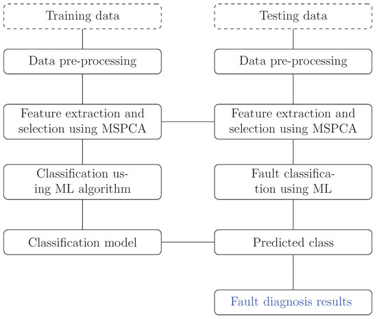
Figure 1.
Illustration of MSPCA-based ML procedure for fault detection and isolation.
2.2. Feature Extraction and Selection Using Multiscale PCA
Considering the data matrix X, collected from a process operating under normal conditions with N samples of m variables, the data is first normalized to zero mean and unit variance
Through the PCA transformer a new matrix of uncorrelated variables has been extracted, representing data features,
where , , P is the loading matrix obtained by an orthogonal transformation of the covariance matrix which can be obtained through eigenvalue decomposition
where is a diagonal matrix contains the eigenvalues sorted in a decreasing order.
Data dimensionality reduction can be achieved by splitting P and into modelled and non-modelled variations, the first one and spanning the principal subspace and the other part is and spanning the residual subspace. The columns of are the eigenvectors of the covariance matrix associated with the first ℓ largest eigenvalues in corresponding to the most variation of the data. ℓ is the number of principal components (PCs). The columns of are the remaining eigenvectors related to eigenvalues in . As a result, PCA decomposes the original data set X into:
With
represents the selected features which are obtained through the projection of X onto the first ℓ eigenvectors corresponding to the largest variances of the sample covariance matrix. In summary, the PCA model is determined based on an eigen-decomposition of the covariance matrix . The obtained PCA model is used to extract and select significant features to be classified. Such features should be conveniently extracted in such a way to emphasize the differences between normal and one or various abnormalities operating conditions.
The MSPCA model was developed by Bakshi [32] with the aim of combining the ability of PCA to extract cross-correlation between variables with the ability of orthonormal wavelets to separate feature from noise and approximately decorrelate autocorrelation between available measurements [32,33]. Some of the advantages of multiscale representation in process modeling and monitoring are presented in [32,34].
Multiscale representation has the ability to separate noise from important features in the data. It helps transform the data to be closer to normal at multiple scales even though their distribution in the time-domain does not follow normal distribution. The benefits of multiscale representation described above legibly present that they can help verify the assumptions of independence, normality and noise level made by PCA model [32]. The main steps in the multiscale PCA model are presented in Algorithm 1 [32].
| Algorithm 1 MSPCA algorithm |
data matrix X, Confidence interval .
|
To obtain a good performance of classification, it is of significance to extract statistical features via MSPCA model by exhaustively enumerating some possible values. In the current study, the selected features extracted from the MSPCA model are the squared prediction error (SPE) statistic [35], the statistic [36], the squared weighted error (SWE) statistic [37] and the first retained principal components ().
2.3. Faults Classification Using Machine Learning (ML) Technique
Machine learning classifiers are adjusted to the most informative features chosen after being extracted and selected from the data for fault classification reasons. These classifiers incorporate decision tree [27], support vector machines (SVM) [28], K-Nearest Neighbors (KNN) [29,30] and Naive Bayes (NB) [31].
Next, an overview of these classifiers is reported.
2.3.1. Decision Trees
A decision tree is one of the most common classifier that has been strongly used in many real-world applications [27,38]. This symbolic learning technique correlate information in a stratified structure obtained from a training dataset consisted of nodes and ramifications. The aim of this classifier is to minimize the least squares error for the next split of a node in the tree, in order to predict the average of the dependent variable of all training instances covered for unseen instances in a leaf. A decision tree model splits the space into J splits the x space into J disjoint regions and predicts a separate constant value in each one as follows:
or equivalently
where is the mean of the response y in each region , , is the size of region . Hence, a tree predicts a constant value within each region . The trees are built using top-down iterative splitting based on a least squares fitting criterion. The guideline of this model is the regions of the partition resolved by the identities of the predictor variables which are utilized for splitting and their corresponding split points.
2.3.2. Support Vector Machines
Next, an introduction of the basic ideas of support vector machines (SVM) for classification is developed. Keep in mind a given training set of N samples , with input data and output that represents a set of labeled training features. The SVM takes the following form:
where and . In order to locate the hyperplanes of linear separation to be as far from the support vectors as possible, the margin defined by should be maximized. It is equivalent to finding:
Allocating the constraints Lagrange multipliers , where , the quadratic programming (QP) optimization problem (9) becomes
by setting the partials of (10), with respect to w and b, to zero
Substituting (11) into (10) gives the dual optimization problem of the primary depending on :
where . The solution of the optimization problem (12) returns to determine . After that, w is easily calculated using (11). In order to determine b, a new data satisfying (11) is presented, and a support vector takes the following form:
Referring to the separation hyperplane equations and regardless the class , the variable b is given by:
In turn, the optimal orientation of the separating hyperplanes is obtained.
2.3.3. K-Nearest Neighbors
The K-nearest neighbors (K-NN) [30] is the most well known machine learning technique in which a non parametric method is used to identify in which class, already known, unidentified data belong to it. The attachment to such class is based on the Euclidean distance to k-nearest neighbors. Taking into account the elements of known class are and those of the data to be classified are , then, the distance is obtained by
A class is designated when the distance determined in Equation (15) is minimal.
2.3.4. Naive Bayes
The Naive Bayes [31] is a probabilistic classifier based on applying Bayes’ theorem of the conditional probability with a strong independence assumption between features. Thus, the assignment of a feature to one of K possible classes is based on the conditional probability value:
As the features are known and mutually independent, doesn’t depend on the class and
Thus,
One common decision-making rule is the maximum a posteriori probability decision rule. The corresponding classifier, a Bayes classifier, is the function which assigns a class label to for some k as follows:
3. Simulation Results
3.1. Application 1: Simulated Synthetic Data
In this simulation example and in order to generate the fault database, we assumed a condition without faults (healthy mode), and conditions with three types of faults considering the manual data analysis (faulty modes). Appropriate multiscale preprocessing of the database was necessary to utilize the generated fault database as learning data for the machine learning. We generated a fault database using the system simulation and labeled the fault based on the simulation results. Labeled data are useful for machine learning methods.
The simulated synthetic example replicates and extends the illustrative example carried out in the original MSPCA paper [32]. Two variables are generated using Gaussian measurements that are uncorrelated, of zero mean and unit variance. The final variables are generated by adding and subtracting the first two variables, respectively, as shown in the following equations [32]:
The measured data matrix, (of six variables), is then contaminated by white noise, that is uncorrelated Gaussian error, of zero mean and standard deviation of as follows [32]:
Normal operating condition consisted of 2048 equally spaced observations. Abnormal operation (also of 2048 observations) consists of a step change in the mean (of size equals 2) in all four variables between samples between observations 512 and 1024 (), variance change between 1025 and 1537 () and incipient fault between 1538 and 2048 () (see Figure 2).
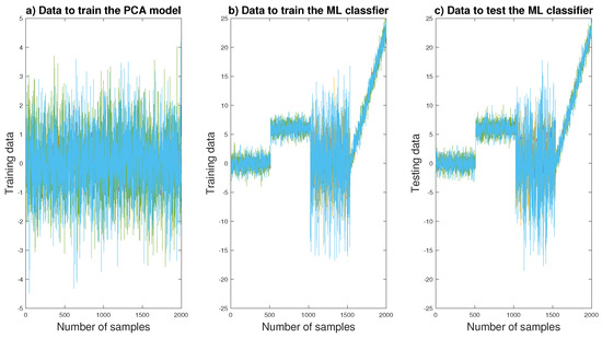
Figure 2.
Data generation of numerical example.
In order to evaluate the different classifiers for FDI purposes, the simulated 6 variables are generated (see Equation (20)). In our study, the main steps used in the data generation are training healthy data generation (Figure 2a), training faulty data generation (Figure 2b) and testing faulty data generation (Figure 2c).
First, under a healthy operating conditions (Figure 2a), the corresponding data set is used to build a PCA model after its normalization to zero mean and unit variance. Through the eigenvalue decomposition, the obtained variances of the transformed variables are sorted in decreasing order. Second, to generate training faulty database, we assumed a conditions with three types of faults considering the manual data analysis (faulty modes) (please refer to Figure 2b). The generated faulty data (called also training data) are used to train the machine learning classifiers. Third, in the testing phase, a new samples are generated using the same model (used in the training phase). These new data (called also testing data) are used to validate the machine learning classifiers (please see Figure 2c).
These variables represent one healthy (assigned to class ) and 3 different faulty operating modes of synthetic data (assigned to ), as reported in Table 1.

Table 1.
Construction of database for fault diagnosis system.
To obtain a good performance of diagnosis -based approaches, it is of significance to extract statistical features via PCA model. In the current study, the selected features extracted from the PCA model are the squared prediction error (SPE) statistic, the statistic, the squared weighted error (SWE) statistic and the first retained principal components. In the current work, 3 arbitrary groups of features are used, including group 1: , group 2: and group 3: (see Table 2).
Table 2.
Selected features for fault classification.
Next, a fault classification framework introduces the extracted and selected features to the several machine learning classifiers. These methods include decision tree (DT), support vector machines (SVM), K-Nearest Neighbors (KNN) and Naive Bayes (NB). They use labeled training data to learn a set of predefined fault classes.
To demonstrate the performance of the DT, SVM, KNN and NB, we adopted a 10-fold cross-validation approach to obtain the accuracy of the classifiers.
In order to have reference results, a Monte-Carlo simulation of 100 runs is performed and used to compute the classification accuracies using DT, SVM, KNN and NB.
Next, the four classifiers (KNN, NB, DT and SVM) are simulated and based on the classification accuracy the best classifier is selected. Table 3 and Table 4 present the global performance accuracy for different selected features and for the used classifiers. It can be clearly seen that the selected features of group 2 ( and statistics) and the features of group 3 (the first PCs) present the best results according to their classification accuracy. In terms of percentage of accuracy, Table 3 and Table 4 show the performances results. It is clear that PCA, MSPCA-based SVM and KNN using group 3 as input features provide best tradeoffs. The accuracy rates have been successfully achieved 91.06%, 92.82% and 94.73%, 93.95% respectively. It can be shown from the results that the MSPCA provides better tradeoffs when compared to the classical PCA.
Table 3.
Accuracies of extracted features based PCA with different classifiers.
Table 4.
Accuracies of extracted features based MSPCA with different classifiers.
We can show from Table 3 and Table 4 that MSPCA-based ML provides better classification accuracy when compared to those using ML based PCA techniques. For example, MSPCA-based KNN through groups 1 to 3 gives 100% of classification accuracy.
To show the classification efficiency of the developed approach under different simulation conditions, we vary for example the fault size of the mean between 1 and 3 and evaluate the performance of MSPCA-based SVM (please refer to Table 5). The obtained results show that the developed MSPCA-based SVM approach still provides a good classification accuracies through the three groups.
Table 5.
Accuracies of extracted features based MSPCA-based SVM with different fault sizes.
3.2. Application 2: Air Conditioning Systems
3.2.1. Description of Air Conditioning Systems
Transient system (TRNsys Simulation Tool, simulation software) with TRNsys Simulation Studio (graphical front-end) and interface TRNBuild have been used to modulate the building and to generate Air Conditioning systems data [39]. Other studies have used TRNSYS software to generate the data [40] and to simulate the buildings faults [41]. TRNBuild interface allows adding the non-geometrical properties such as door and window properties, layer and wall material properties, thermal conductivity and different gains etc.
For the building in TRNSYS (see Figure 3), we build a detailed three-zone building model using Type 56, which constructs all the layers of floors, walls and ceilings with their physical properties such as conductivity, density and specific capacitance as well as detailed window models.

Figure 3.
TRNsys model.
Table 6 presents a summary of the set-up for the building. Based on this table, a building model is developed in TRNSYS. The type- 56 multi-zone building is a reproduction of the reference building. The building model is divided into 3 zones. Air Conditioning is supplied locally in each room by electric air conditioning; the buildings have no heating system. However, the recommended set point for cooling is equal to 26 C. The TRNSYS model has been run using the existing building parameters described earlier, with 1 h time step, using the U. S. Department of Energy (DOE) typical meteorological year version 2 (TMY2) weather data [42].
Table 6.
Brief description of the base building parameters for simulation.
A simulation based case study was set up to demonstrate the FDI system. Three rooms are modeled in TRNSYS. The rooms are simulated with different load profiles and schedules. One room is monitored for FDI in this study. The model is assumed to be located in Doha-Qatar. The simulations are conducted for the Air Conditioning season due to the Air Conditioning dominated weather. One year of normal operation data is used to train and set up the FDI system.
In the current study and under a healthy operating conditions, the corresponding data set is used to build a PCA model after its normalization to zero mean and unit variance. Through the eigenvalue decomposition, the obtained variances of the transformed variables are sorted in decreasing order. According to the most significant captured information in the data via its projection, a PCA model with three directions has been constructed. In fact, this selection is based on that the variance of obtained component less or equal to one characterizes noise and measurement error. This is confirmed by the minimization of the reconstruction error variance. To generate fault database, we assumed a condition without faults, and conditions with two types of faults. The two fault cases are generated in TRNSYS, including the zone level operation faults. The faults occur individually and are implemented statically by altering existing objects such as schedules in TRNSYS. The two faults are described as follows:
- Unplanned occupancy is considered an abnormal occupation, i.e., a presence of unplanned occupant different from occupancy desired profile or more occupants present than allowed. This fault is simulated by injecting unplanned occupants.
- Opening a window while the Air Conditioning system is operating is an example of a fault that is generated by an occupant and causes wastage of energy sources.
Usually, building operational performance is measured in terms of comfort, system efficiency, productivity, environmental quality, and functionality. Unplanned occupancy as well opening window will increase energy consumption and cost. Simulation data explain how extra air conditioning power appears because of unplanned occupancy or opening window. It also represents the variations in indoor temperature. For example, opening a window might increase the air quality level but at the same time it might decline indoor thermal comfort.
As the FDI problem can be seen as a classification problem, there are totally three classes of data used here: one class of fault free data and two classes of faulty data. The time range of the data is from 0 h to 8760 h (1 year) with 1h time step (the dataset can be found at the link: https://www.kaggle.com/sondesgharsellaoui/fdi-dataset). The generated data extracted from Air Conditioning systems are presented in Figure 4.

Figure 4.
Data generation of air conditioning systems data.
In many cases, data does not represent the real values of actions. Furthermore, there are various factors are linked to each other and occupants are unable to choose the right actions. For example, closing a window might improve indoor thermal comfort but at the same time, it might reduce the air quality level. Similarly, cooling load is very sensitive to outdoor temperature and often it is not connected to future energy consumption load. Generally, the energy consumption of the air conditioner depends on several external factors such as outdoor temperature, humidity, wind velocity, atmospheric pressure (please refer to Table 7).
Table 7.
Variables description.
3.2.2. Fault Classification Results
Again, to evaluate the performance of the four classifiers, a 10-fold cross-validation is employed. In order to carry out the the proposed FDI approach, various simulated 5 variables measurements are collected (see Table 7). These variables represent one healthy (assigned to class ) and 2 different faulty operating modes (assigned to ), as presented in Table 8. In this case study, 3 groups of features are used, including group 1: , group 2: and group 3 (see Table 2).
Table 8.
Construction of database for fault diagnosis system.
Table 9 and Table 10 present the global performance accuracy for different selected features and for the applied classifiers. From these tables it is clear that the selected features of group 2 ( and statistics) and features of group 3 (the first PCs) give the best compromise in terms of classification accuracy. Performance results in terms of percentage of accuracy are reported in Table 9 and Table 10. It is clear that the results using SVM and KNN techniques through group 3 provide the best tradeoffs. The accuracy rates have been successfully achieved 89.17%, 90.70% and 99.08%, 100% respectively.
Table 9.
Accuracies of extracted features based PCA with different classifiers.
Table 10.
Accuracies of extracted features based MSPCA with different classifiers.
4. Conclusions
In this paper, the problem of Fault Detection and Isolation (FDI) of Air Conditioning Systems (AC) has been addressed. The developed technique is based on the machine learning (ML)-based Multiscale Principal Component Analysis (MSPCA). The developed MSPCA-based ML approach is addressed so that the MSPCA technique was used for feature extraction and selection purposes and the ML technique is applied for faults diagnosis. The proposed approach was developed for systems monitoring under normal and faulty conditions. Different cases were investigated in order to show the robustness and the efficiency of the developed approach. The effectiveness of the FDI approach was studied using a synthetic and simulated Air Conditioning systems data. The high detection and monitoring accuracy presented a good impact on the energy production in Air Conditioning systems. Under different simulation conditions, the developed FDI technique showed a good monitoring condition and higher detection accuracy. As a conclusion, the proposed fault detection and isolation method can help to maintain the comfort and reduce energy consumption.
There are a number of threats that may have an impact on the results of this study. The fault detection and isolation approaches proposed in this study were built by using default parameters. That is, we have not investigated how these approaches are affected by varying the parameters. Thus, other approaches might be better in monitoring and diagnosing the faults.
The feature extraction approach proposed in the current work is based on the PCA model, which assumes that the relationship between the variables is linear. The next research direction is to extend the current work to achieve further improvements and widen the applicability of the developed method in practice by using the kernel PCA method. The kernel PCA is derived from the nonlinear case of PCA algorithm and it will be investigated as feature extraction algorithm in the task of fault detection and isolation.
Additionally, in the current work, we assumed that the features are single-valued data represented, however, a more accurate monitoring and diagnosis can be obtained by representing the uncertainties in the systems by using interval-valued data representation. As future work, we plan to extend the current work to interval-valued data feature extraction based machine learning for detection and diagnosis purposes.
Author Contributions
S.G. established the major part of the present work which comprises modeling, simulation and analyses of the obtained results. M.M., S.S.R., H.A.-R., H.M. have earnestly contributed to verifying the work and finalizing the paper. All authors have read and agreed to the published version of the manuscript.
Funding
This work was supported by the Qatar National Research Fund (a member of the Qatar Foundation) under Grant [NPRP10-0101-170082] and by IBERDROLA QSTP LLC.
Acknowledgments
This publication was made possible by NPRP grant [NPRP10-0101-170082] from the Qatar National Research Fund (a member of Qatar Foundation) and the co-funding by IBERDROLA QSTP LLC. The statements made herein are solely the responsibility of the authors.
Conflicts of Interest
The authors declare no conflict of interest.
References
- Saffouri, F.; Bayram, I.S.; Koç, M. Quantifying the cost of cooling in qatar. In Proceedings of the 2017 9th IEEE-GCC Conference and Exhibition (GCCCE), Manama, Bahrain, 8–11 May 2017; pp. 1–9. [Google Scholar]
- Najeh, H.; Singh, M.P.; Chabir, K.; Ploix, S.; Abdelkrim, M.N. Diagnosis of sensor grids in a building context: Application to an office setting. J. Build. Eng. 2018, 17, 75–83. [Google Scholar] [CrossRef]
- Elnour, M.; Meskin, N.; Al-Naemi, M. Sensor data validation and fault diagnosis using Auto-Associative Neural Network for HVAC systems. J. Build. Eng. 2020, 27, 100935. [Google Scholar] [CrossRef]
- Frank, S.M.; Kim, J.; Cai, J.; Braun, J.E. Common Faults and Their Prioritization in Small Commercial Buildings: February 2017-December 2017; Technical Report; National Renewable Energy Laboratory (NREL): Golden, CO, USA, 2018.
- Pérez-Lombard, L.; Ortiz, J.; Pout, C. A review on buildings energy consumption information. Energy Build. 2008, 40, 394–398. [Google Scholar] [CrossRef]
- Lin, Y. Modeling the Thermal Dynamics of a Single Room in Commercial Buildings and Fault Detection. Ph.D. Thesis, University of Florida, Gainesville, FL, USA, 2012. [Google Scholar]
- Radhakrishnan, R.; Nikovski, D.; Peker, K.; Divakaran, A. A comparison between polynomial and locally weighted regression for fault detection and diagnosis of hvac equipment. In Proceedings of the IECON 2006—32nd Annual Conference on IEEE Industrial Electronics, Paris, France, 6–10 November 2006; pp. 3668–3673. [Google Scholar]
- Zaheeruddin, M.; Tudoroiu, N. Dual EKF estimator for fault detection and isolation in Heating Ventilation and Air Conditioning systems. In Proceedings of the IECON 2012—38th Annual Conference on IEEE Industrial Electronics Society, Montreal, QC, Canada, 25–28 October 2012; pp. 2257–2262. [Google Scholar]
- Tudoroiu, N.; Zaheeruddin, M. Joint UKF estimator for fault detection and isolation in Heating Ventilation and Air Conditioning systems. In Proceedings of the 2011 5th International Symposium on Computational Intelligence and Intelligent Informatics (ISCIII), Floriana, Malta, 15–17 September 2011; pp. 53–58. [Google Scholar]
- Du, J.; Er, M.J. An artificial intelligence approach towards fault diagnosis of an air-handling unit. In Proceedings of the 2004 5th Asian Control Conference (IEEE Cat. No. 04EX904), Melbourne, VIC, Australia, 20–23 July 2004; Volume 3, pp. 1594–1601. [Google Scholar]
- Dexter, A.; Pakanen, J. Energy Conservation in Buildings and Community Systems—Annex 34; International Energy Agency: Paris, France, 2006. [Google Scholar]
- Ding, S.X. Model-Based Fault Diagnosis Techniques: Design Schemes, Algorithms, and Tools; Springer Science & Business Media: Berlin/Heidelberg, Germany, 2008. [Google Scholar]
- Isermann, R. Model-based fault-detection and diagnosis–status and applications. Annu. Rev. Control 2005, 29, 71–85. [Google Scholar] [CrossRef]
- Reddy, T.A.; Niebur, D.; Andersen, K.K.; Pericolo, P.P.; Cabrera, G. Evaluation of the suitability of different chiller performance models for on-line training applied to automated fault detection and diagnosis (RP-1139). HVAC&R Res. 2003, 9, 385–414. [Google Scholar]
- Du, Y.; Du, D. Fault detection and diagnosis using empirical mode decomposition based principal component analysis. Comput. Chem. Eng. 2018, 115, 1–21. [Google Scholar] [CrossRef]
- Schein, J.; Bushby, S.T.; Schein, J.R. A Simulation Study of a Hierarchical, Rule-Based Method for System-Level Fault Detection and Diagnostics in HVAC Systems; US Department of Commerce, National Institute of Standards and Technology: Gaithersburg, MD, USA, 2005.
- Fernando, H.; Surgenor, B. An unsupervised artificial neural network versus a rule-based approach for fault detection and identification in an automated assembly machine. Robot. Comput.-Integr. Manuf. 2017, 43, 79–88. [Google Scholar] [CrossRef]
- Trothe, M.E.S.; Shaker, H.R.; Jradi, M.; Arendt, K. Fault Isolability Analysis and Optimal Sensor Placement for Fault Diagnosis in Smart Buildings. Energies 2019, 12, 1601. [Google Scholar] [CrossRef]
- Fezai, R.; Mansouri, M.; Abodayeh, K.; Nounou, H.; Nounou, M. Online reduced gaussian process regression based generalized likelihood ratio test for fault detection. J. Process Control 2020, 85, 30–40. [Google Scholar]
- Jolliffe, I.T. A note on the use of principal components in regression. J. R. Stat. Soc. Ser. C (Appl. Stat.) 1982, 31, 300–303. [Google Scholar] [CrossRef]
- Harkat, M.F.; Mourot, G.; Ragot, J. An improved PCA scheme for sensor FDI: Application to an air quality monitoring network. J. Process Control 2006, 16, 625–634. [Google Scholar] [CrossRef]
- Kuncheva, L.I.; Faithfull, W.J. PCA feature extraction for change detection in multidimensional unlabeled data. IEEE Trans. Neural Netw. Learn. Syst. 2013, 25, 69–80. [Google Scholar] [CrossRef] [PubMed]
- Ren, L.; Xu, Z.; Yan, X. Single-sensor incipient fault detection. IEEE Sens. J. 2010, 11, 2102–2107. [Google Scholar] [CrossRef]
- Kouadri, A.; Hajji, M.; Harkat, M.-F.; Abodayeh, K.; Mansouri, M.; Nounou, H.; Nounou, M. Hidden Markov model based principal component analysis for intelligent fault diagnosis of wind energy converter systems. Renew. Energy 2020, 150, 598–606. [Google Scholar] [CrossRef]
- Fazai, R.; Mansouri, M.; Abodayeh, K.; Puig, V.; Noori Raouf, M.-I.; Nounou, H.; Nounou, M. Multiscale Gaussian process regression-based generalized likelihood ratio test for fault detection in water distribution networks. Eng. Appl. Artif. Intell. 2019, 85, 474–491. [Google Scholar] [CrossRef]
- Fazai, R.; Abodayeh, K.; Mansouri, M.; Trabelsi, M.; Nounou, H.; Nounou, M.; Georghiou, G.E. Machine learning-based statistical testing hypothesis for fault detection in photovoltaic systems. Sol. Energy 2019, 190, 405–413. [Google Scholar] [CrossRef]
- Quinlan, J.R. Simplifying decision trees. Int. J. Man-Mach. Stud. 1987, 27, 221–234. [Google Scholar] [CrossRef]
- Cortes, C.; Vapnik, V. Support-vector networks. Mach. Learn. 1995, 20, 273–297. [Google Scholar] [CrossRef]
- Suguna, N.; Thanushkodi, K. An improved k-nearest neighbor classification using genetic algorithm. Int. J. Comput. Sci. Issues 2010, 7, 18–21. [Google Scholar]
- Wang, Y.; Pan, Z.; Pan, Y. A Training Data Set Cleaning Method by Classification Ability Ranking for the k-Nearest Neighbor Classifier. IEEE Trans. Neural Netw. Learn. Syst. 2019. [Google Scholar] [CrossRef]
- Jiang, L.; Zhang, L.; Yu, L.; Wang, D. Class-specific attribute weighted naive Bayes. Pattern Recognit. 2019, 88, 321–330. [Google Scholar] [CrossRef]
- Bakshi, B. Multiscale PCA with application to multivariate statistical process monitoring. AIChE J. 1998, 44, 1596–1610. [Google Scholar] [CrossRef]
- Li, X.; Zhang, X.; Zhang, P.; Zhu, G. Fault Data Detection of Traffic Detector Based on Wavelet Packet in the Residual Subspace Associated with PCA. Appl. Sci. 2019, 9, 3491. [Google Scholar] [CrossRef]
- Ganesan, R.; Das, T.K.; Venkataraman, V. Wavelet-based multiscale statistical process monitoring: A literature review. IIE Trans. 2004, 36, 787–806. [Google Scholar] [CrossRef]
- Dunia, R.; Qin, S.J.; Edgar, T.F.; McAvoy, T.J. Identification of faulty sensors using principal component analysis. AIChE J. 1996, 42, 2797–2812. [Google Scholar] [CrossRef]
- Qin, S.J.; Dunia, R. Determining the number of principal components for best reconstruction. J. Process Control 2000, 10, 245–250. [Google Scholar] [CrossRef]
- Qin, S.J.; Li, W. Detection, identification, and reconstruction of faulty sensors with maximized sensitivity. AIChE J. 1999, 45, 1963–1976. [Google Scholar] [CrossRef]
- Steinberg, D.; Colla, P. CART: Classification and regression trees. Top Ten Algorithms Data Min. 2009, 9, 179. [Google Scholar]
- Klein, S.; Beckman, W.; Mitchell, J.; Duffie, J.; Duffie, N.; Freeman, T.; Mitchell, J. TRNSYS 17: A Transient System Simulation Program; Solar Energy Laboratory, University of Wisconsin: Madison, WI, USA, 2010. [Google Scholar]
- Muñoz, I.; Cortés, F.; Crespo, A.; Ibarra, M. Development of a failure detection tool using machine learning techniques for a large aperture concentrating collector at an industrial application in Chile. AIP Conf. Proc. 2019, 2126, 170008. [Google Scholar]
- Singh, M.; Kien, N.T.; Najeh, H.; Ploix, S.; Caucheteux, A. Advancing Building Fault Diagnosis Using the Concept of Contextual and Heterogeneous Test. Energies 2019, 12, 2510. [Google Scholar] [CrossRef]
- Marion, W.; Urban, K. User’s Manual for TMY2s, Typical Meteorological Years, Derived from the 1961-1990 National Solar Radiation Data Base; Technical Report, NREL/SP-463-7668; National Renewable Energy Laboratory (NREL): Golden, CO, USA, 1995.


© 2020 by the authors. Licensee MDPI, Basel, Switzerland. This article is an open access article distributed under the terms and conditions of the Creative Commons Attribution (CC BY) license (http://creativecommons.org/licenses/by/4.0/).