Abstract
In this paper, the approximation of a fractional-order PIDcontroller is proposed to control a DC–DC converter. The synthesis and tuning process of the non-integer PID controller is described step by step. A biquadratic approximation is used to produce a flat phase response in a band-limited frequency spectrum. The proposed method takes into consideration both robustness and desired closed-loop characteristics, keeping the tuning process simple. The transfer function of the fractional-order PID controller and its time domain representation are described and analyzed. The step response of the fractional-order PID approximation shows a faster and stable regulation capacity. The comparison between typical PID controllers and the non-integer PID controller is provided to quantify the regulation speed introduced by the fractional-order PID approximation. Numerical simulations are provided to corroborate the effectiveness of the non-integer PID controller.
1. Introduction
A power converter is a device that transforms the power supply characteristics into the ones required by a particular machine; DC–DC conversion is one of the most known applications [1]. Research into DC–DC converters involves plenty of techniques proposed to improve performance [2], efficiency [3,4] and modeling [5] or to reduce conduction losses [6], to mention a few.
Different control strategies have been proposed to enhance performance of DC–DC converters, ranging from the widely used Proportional-Integral and Proportional-Integral-Derivative controllers [7,8,9], sliding mode control [10], passivity-based control [11], fuzzy logic controllers [12,13] or poles placement [14], for instance.
In the last decade, control strategies have been explored, redesigned and adapted from the fractional calculus perspective, mainly seeking to improve the modeling accuracy and dynamic response. The main reasons behind using fractional calculus can be summarized as follows [15,16,17]:
- Lower order derivatives implies lower (reduction) levels of noise.
- Robustness against parameters variations.
- Better description of systems due to an extra degree of freedom (the fractional order).
- Fits better the frequency behavior of some systems.
- Fractional relations are realizable through ladder, trees or fractal arrangements of traditional electronic elements.
- Good description of long-term memory effects, non-locality and fractal properties of systems.
- Exact (good) approximation of systems with lumped (distributed) parameters.
- Flexibility to approximate systems with large dimensional nature.
Many remarkable results, reporting the synthesis of non-integer order controllers for power converters, have shown the effectiveness of fractional calculus in Control Theory. In [18], the non-ideal model of a DC–DC converter is controlled through an Internal Model Control strategy, which encapsulates the model of the plant within the controller, resulting in a structure resembling a PID with an extra lag network. The fractional-order controller improved the steady state performance. In [19], a fractional-order PI controller is combined with fuzzy-logic precompensators to control a Buck converter via capacitor current. The combination improved the system disturbance-rejection capability and reference tracking performance. In [20], a type-II fuzzy PID controller is proposed to handle uncertainties and external disturbances in a DC–DC converter connected to a microgrid. It minimized the instability effects in the converter, caused by the constant power loads of the microgrid. To improve the performance with respect to the varying parameters, an optimization algorithm for tuning the controller coefficients was proposed as well. A fractional-order back–stepping sliding mode controller was suggested in [21]. The controller showed robustness regulating voltage of DC–DC converters in presences of uncertainties, unmodeled dynamics and non-linear loads. Moreover, it improved the capability of perturbation rejection and reduced the steady-state error. In a similar approach, an adaptive fractional-order sliding mode control was designed for current tracking for a DC–DC converter in [22]. The adaptation rules were based on state observers and Lyapunov functions. Good transient response and robustness were the most important improvements. In [23], a fractional-order PID controller was suggested to stabilize a DC-bus voltage of a ultra-capacitor hybrid energy system. An optimization algorithm was suggested to tune the controller parameters. The steady-state response showed higher performance and better steady-state properties. In [24], a fractional-order PID controller was used to regulate the output voltage of a DC–DC converter in a photovoltaic (PV) system. The integration of incremental conductance method, maximum power point tracking and root locus technique was suggested to compute the controller parameters. This combination resulted in fast dynamics and high tracking accuracy under severe climate variations.
The above reviewed results showed that fractional-order controllers successfully achieved the control objectives and outperformed integer-order ones, yet they present two main drawbacks. On one hand, the controllers were designed by using one of the following definitions of the integro-differential operator: Grünwald–Letnikov, Riemann–Liouville or Caputo [25,26,27], which increase the computational and implementation complexity. On the other hand, the parameters of controllers were obtained by either bee swarm, ant colony, bat, flower pollination, Nelder–Mead or teacher-learning optimization algorithms, which required the control strategy to be adapted to them, increasing the computational complexity.
In this paper, a simpler procedure to approximate a fractional-order PID controller to regulate the output voltage of a DC–DC Buck converter is explored. The non-integer approach is suggested due to fractional calculus have demonstrated accuracy in modeling real systems/phenomena and robustness against parameter variations. It is proposed to approximate the controller through a method that employs a frequency approach, the result of which is a controller that exhibits a flat phase response in a band-limited frequency spectrum. The proposed method takes into consideration both robustness and desired closed-loop characteristics, keeping the tuning process simple. It is shown that the resulting structure of the controller allows obtaining its representation in the time domain, which makes it easier to analyze its effects in transient and permanent regimes.
The paper is organized as follows: Section 2 provides with the necessary preliminaries on DC–DC buck converter, i.e., its basic operation and the model description are provided. The method to be used to approximate the fractional-order PID controller is given in this section as well. In Section 3 the synthesis of the fractional-order PID controller is described step by step. The tuning process of the fractional-order PID controller and the numerical results are also provided in this section. A comparison of performance and robust stability of typical PID controllers vs the fractional-order PID controller is addressed in this section as well. In Section 4 the proposal for the possible realization of the fractional-order PID controller is described. Discussion and conclusions on the presented numerical results are provided in Section 5 and Section 6, respectively.
2. Materials and Methods
In this section preliminaries on DC–DC Buck converter and its modeling are provided. The method to approximate fractional-order Laplacian operator is also described in this section.
2.1. Buck Converter
A DC–DC converter is an electronic device that provides a variable, but continuous source of voltage from a fixed power supply. The Buck configuration, whose main characteristic is to produce an average output voltage lower than the power supply, is mainly applied as regulated source of power or to control velocity of DC motors.
The electrical diagram of a Buck converter is shown in Figure 1a, whose basic elements are: a DC voltage source , a capacitor C, an inductance L, a resistor R and two complementary switches and , i.e., when is on, is off and vice versa. Figure 1a with switches and is commonly implemented as shown in Figure 1b with G and D, respectively.
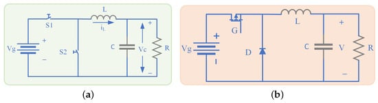
Figure 1.
(a) Electrical representation of the converter. (b) Electrical diagram describing the way a Buck converter is implemented.
The ideal operation in continuous conduction mode (CCM) of the circuit from Figure 1a can be divided into two modes. During mode 1, is on and is off at , current reaches the load R flowing through and the inductance L. The operating mode 1 is described as follows [1,28],
During mode 2, is on and is off at , the inductor current flows through , decaying until is activated again. The operating mode 2 is described as follows [1,28],
A continuous time–invariant linear model of Buck converter can be derived from the nonlinear time–variant circuit of the converter (1) and (2), over one period T of duty cycle D, shown in Figure 2, as follows [1,28],
where is the average of duty cycle D. Considering that is the output of the system and is the control input , the transfer function of system (3) is described by,
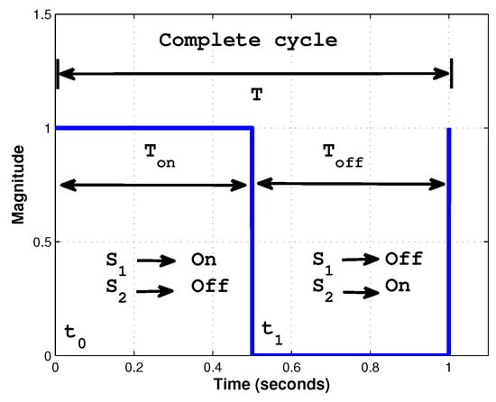
Figure 2.
Duty cycle for the Buck converter on Figure 1, producing the described operating modes.
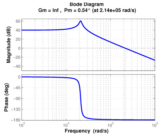
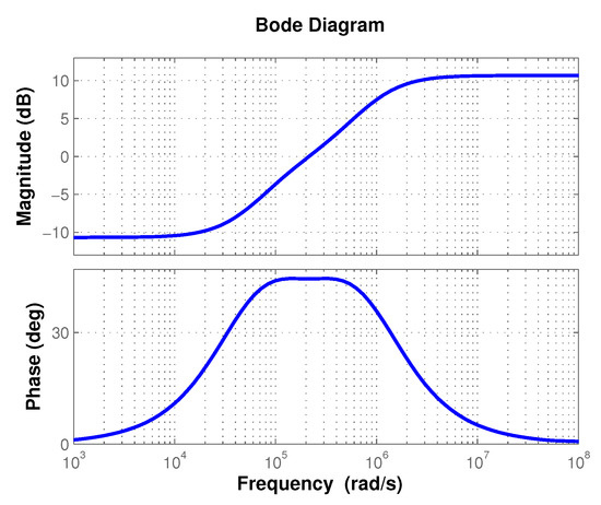
Parameters shown in Table 1 have been used to implement a Buck converter in [29]. The converter showed good performance operating at a switching frequency kHz in continuous conduction mode for microgrids with constant power loads. By using those values, (4) exhibits the frequency response shown in Figure 3.

Table 1.
Component values of Buck converter from Figure 1.
In the next section the approximation of the fractional-order PID controller is performed.
2.2. Fractional-Order Approximation of Laplacian Operator
In the following, the method used to approximate the Laplacian operator is summarized.
El-Khazali method uses biquadratic modules with flat phase response to approximate the integro–differential operator , where . The fractional derivative operator can be approximated by El-Khazali method as follows [30,31],
where is the center frequency and , , are real constants defined as,
For and , , which means that (5) behaves as a fractional-order differentiator around the center frequency [30]. The phase flatness of (5), is guaranteed as long as [30,31]
In the following section, numerical simulation and a comparison between integer/fractional-order controllers will be shown.
3. Results
In this section, the synthesis and tuning of an approximation of a fractional-order PID controller is described. Performance results are presented through numerical simulations.
3.1. Synthesis and Tuning of Fractional-Order PID Controller
The fractional-order PID controller is described as [32]
where , is the proportional gain, and are the integral and derivative time constants, respectively. If one obtains the integer–order PID controller, which was studied through loop shaping and optimization to find, among other characteristics, the influence of relation in frequency design approach, where is a constant in order to obtain a unique solution [33,34]. By setting , and a slightly modification on (8) to achieve a perfect square trinomial [35], (8) becomes,
where . With the appropriate combination of and , the closed-loop system, with the open-loop transfer function , should exhibit the desired frequency/time response.
The relationship between the desired phase margin and the phase of the controller–plant pair is , where and are the controller and plant phase contribution, respectively, implying that
If (5) is manipulated as and substituted into (9), as (), which is the fractional-order differentiator (integrator), thus, .
The parameters and will be computed as follows [30], aiming to obtain the starting point for the tuning process,
where to prevent the denominator to be zero. On the other side, by solving (9) using (5), the controller gain is obtained as follows,
where is the phase crossover frequency and must no be 0 or ∞, if so, a large value must be chosen instead [30].
In the following section, the approximation of the fractional-order controller will be computed.
3.2. Numerical Results
Consider the closed-loop diagram of Figure 4, where the plant (4) describes the transfer function of the Buck converter of Figure 1 with the component values of Table 1. The controller design comprises the following steps:
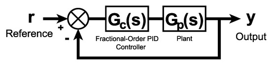
Figure 4.
Closed-loop control diagram considered to regulate the voltage of the DC–DC Buck converter of the Figure 1.
- Investigate the stability margins of the uncontrolled plant.
- Compute the fractional-order of the controller.
- Determine the phase contribution of the controller .
- Determine the integral time constant .
- Determine the controller gain .
- Compute open– and closed-loop transfer functions, evaluate stability and stability margins.
- If stability margins were not met, from the obtained values, slightly move up/down until the desired margins are met.
Reasonable values of phase margin for the system to exhibit acceptable robustness are suggested between 30–60[36]. In this particular case, it is desired the closed-loop system to exhibit a frequency response with the following margins: and .
The stability margins of the uncontrolled plant described by (4), whose frequency response is shown in Figure 3, are and . The phase margin is computed as , where , thus .
By using (11), the corresponding fractional-order for the approximation is , which produces the frequency response shown in Figure 5 obtained with (5) and (6). The phase contribution of the controller , computed by using (10), is consistent with the phase plot of Figure 5.
The integral time constant and the controller gain were computed according to (12) and (13), respectively, where dB, since .
The values above described do not produce the required closed-loop stability margins, since and . By using the obtained values of and as starting point, it was found that the desired stability margins are met with and as shown in Figure 6, which were reached by using the approximation of fractional-order controller described by
where , , , , and , , , , .
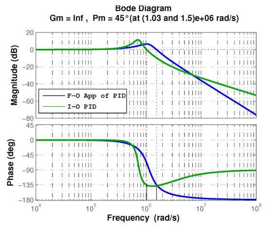
Figure 6.
Frequency response of closed-loop transfer function of a Buck converter when using integer–order PID (green) and fractional-order PID (blue).
In order to show the effectiveness of the fractional-order approximation, the step response of the closed-loop transfer function is depicted in Figure 7.
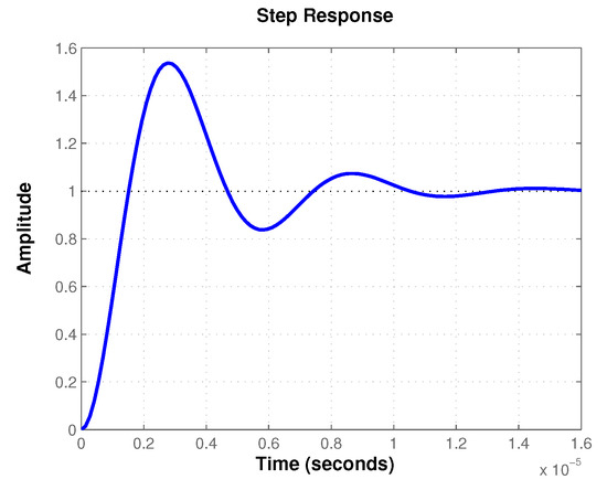
Figure 7.
Step response of the closed-loop transfer function of a Buck converter by using the approximation of the fractional-order PID controller (14).
Figure 7 shows that it took the output an approximate of s to reach the reference, thus, the proposed approximation of fractional-order PID controller would regulate properly the output voltage.
Figure 8 shows the desired output voltage and the inductor current for three different values of reference on Figure 4, i.e., , , and the corresponding control laws, produced by the fractional-order approximation of PID controller (14). As can be seen, for the three conditions of reference r, it took to the fractional-order PID controller to make the plant to reach the desired value of voltage in a very small period of time. On the other side, one can see that the control signals on Figure 8b converged to their expected value of average Duty cycle for each condition of r, i.e., , respectively.
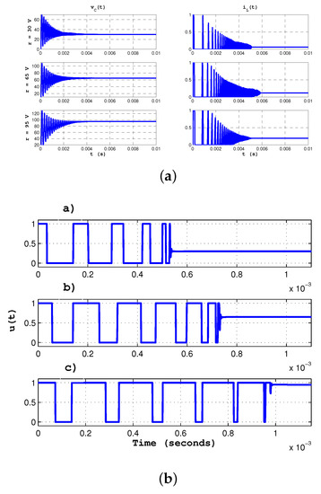
Figure 9 shows the output voltage and inductor current of Buck converter from Figure 1 for reference and different values of the load . One can conclude that the fractional-order PID approximation (5) regulates properly with load variations, which implies robustness of the controller. As can be seen, four load changes were introduced during the process and they all were overcome by the fractional-order PID controller with an amplitude of variation not greater than .
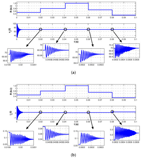
Figure 9.
(a) Output voltage subject to load variations. (b) Inductor current subject to load variations.
3.3. Comparison with Integer–Order PID Controllers
Looking to determine the advantages of employing the approximation of a fractional-order PID controller, typical PID were synthesized and tuned based on two scenarios: the former, considering frequency domain approach, a PID controller was designed seeking to meet a compromise between stability margins and performance; the latter, ensuring stability by shaping the closed-loop characteristic polynomial as a Hurwitz polynomial [37] is obtained by equating the characteristic polynomial with the desired one given by , for .
The PID parameter values are for the first option and for the second option, where . Due to the design values of the converter in Table 1, parameters have to be chosen to ensure the system to be stable.
Figure 10 shows the step response of both integer–order PID controllers. Frequency response of the closed-loop system with the PID controller designed in frequency domain is shown in green in Figure 6.
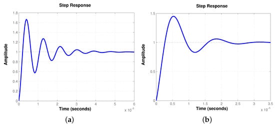
Figure 10.
Step response of the closed-loop transfer function of a Buck converter by using typical PID controllers. (a) PID controller designed in frequency domain. (b) PID controller designed to ensure stability.
The performance parameters of the output voltage by using the three option of controllers are summarized in Table 2, from which one can characterize the response and regulation speed. Comparing data from Table 2, it is easy to note that the approximation of fractional-order PID controller produces a faster response than the one produced by the typical ones, since rising time and settling time from third column are smaller than the corresponding ones in fourth and fifth column. Time constant and peak time have similar behavior. It is important to highlight from Table 2 that even when the time constant and rising time are slightly different, it took the typical PID controllers three times and twice, respectively, the time of the fractional-order PID approximation to settle the control variable.
On the other hand, the output produced by the fractional-order approximation of PID controller exhibits a steady state error that can be neglected due to its magnitude. The overshoot seems to be the only disadvantage, due to it cannot be reduced beyond with acceptable values of .
The time domain representation of the fractional-order PID controller (14) is given as follows,
where the constant and exponent values are provided in Table 3.
Table 3.
Constant and exponent values of the fractional-order PID controller in time domain.
Analyzing (15), one can note that the structure of the fractional-order PID controller will change, since four of its elements will vanish as time passes, remaining only. Thus, for this particular case, the computed fractional-order PID controller approximation has a proportional effect in time domain, which corresponds with the presence of error in steady–state. Additionally, the constant and exponent magnitudes of (15) produce a fast control law, causing the transient of the output to occur in a very short period of time, making the whole system ideal for analog implementation. It is important to mention that, even when the vanishing terms reach zero in a very short period of time, their contribution is fundamental in that interval, since omitting them causes a non desired response.
Lastly, in order to determine the robustness of the closed-loop system for every PID controller, Mu Analysis is performed [38], which computes the structured singular value bounds, where is the set of possible uncertainties. The analysis provides information about the magnitude of the uncertainty that destabilizes the system and the frequency where this occurs. For this particular case, the uncertainty in the parameters will be considered ±30% their nominal value. Figure 11 depicts the upper (solid lines) and lower (dotted lines) bounds of for every PID controller. The minimum of the stability margin is presented at the peak of , thus, the system can resist up to 89% of increase in the uncertainty and still maintain stability.
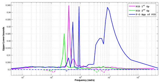
Figure 11.
Upper (solid lines) and lower (dotted lines) bounds of the structured singular value to determine robust stability margins of the closed-loop systems.
4. Proposal for Practical Realization of Fractional-Order PID Controller
A non-integer rational transfer function (RTF) can include fractional integral and derivative terms, which can be positive or negative [39]. Practical implementation of RTF in a physical test–bed requires initially those terms to be approximated as a rational function of two integer–order polynomials within a desired frequency band. The methods developed to perform this approximation can be divided in (a) continue fractional expansion (CFE) and (b) interpolation techniques [40]. For , one can find the Carlson’s, the Matsuda’s and CRONE methods, among others. For , one can find the Outsaloup’s, the refined Outsaloup’s, the Chareff’s methods and the technique recently reported in [41]. Once the approximation process has been performed, the synthesis of the RTF can be obtained. This is generally performed by using either: (a) continue fractional expansion (also known as the ladder or paralleled form), (b) partial fractional expansion (also known as the tree fractance or cascaded parallel) or (c) a combination of both. After processing the approximation and synthesis, the electrical circuit can be obtained. To this end, there are two main approaches, analog and digital [40]. The first one uses resistors, capacitors and operational amplifiers (OPAM), and the second employs FPGA boards.
In this paper, an analog realization is illustrated. By substituting , and in (9) and solving, the fractional-order PID controller one can obtain,
For the approximation stage, the toolbox ninteger was used [42]. The process to obtain the fractional PID approximation is shown in Appendix A. The obtained transfer function after the MATLAB function residue execution [43] is rewritten as follows:
The process to obtain the fractional-order PID synthesis is described in Appendix B. The analog equivalence of (17) is given on basic OPAM configurations (adder, integral, gain), and it is shown in Figure 12. The section on top corresponds to the first fractional integral equivalent (left to right), the section in the middle corresponds to the second fractional integral equivalent (left to right), the bottom one relies to the gain, and the right section (red) refers to the adding points. Parameters of Figure 12 are given in Table 4.
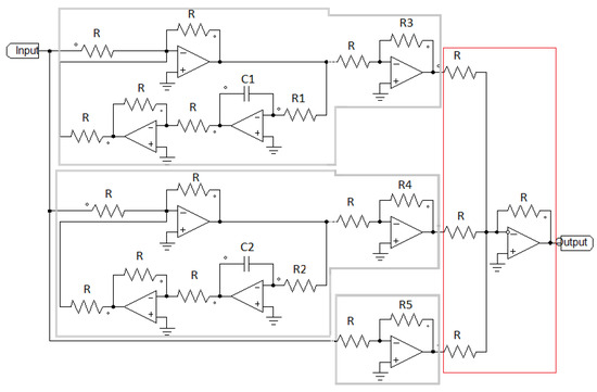
Figure 12.
Electrical circuit with OPAMs for the fractional-order PID controller (17).
Table 4.
Parameter values for the electrical circuit with OPAMs of Figure 12.
By looking Table 4, it can be noticed the particular value of the capacitor, which is high compared to the usual values given in mili or micro Farads. Nowadays, due to the development of super–capacitance technology, it is easy to find and available in the market [44].
5. Discussion
This paper addresses the synthesis and tuning of the approximation of a fractional-order PID controller. Fractional-order approach is used due to it has been proven that controllers of non-integer order outperformed integer–order ones. However, the fractional integro–differential operator is described by either the Grünwald–Letnikov, Riemann–Liouville or Caputo definition, combined with different optimization algorithms to approximate the parameters of the controller. This results in an increase of computational and implementation complexity, which are the main drawbacks of that proposal.
The design process of the controller suggested in this paper considers a frequency domain approach. The approximation is achieved through biquadratic modules with flat phase response, which is used to generate the iso–damping characteristic to bear gain variations. The controller design takes into consideration both robustness and desired closed-loop characteristics, keeping the tuning process simple.
The resulting approximation of fractional-order PID controller produces a notable response with very fast speed of regulation. A comparison with integer–order PID controllers, one designed in frequency domain to meet the same gain and phase margins and the other to ensure stability of the closed-loop system, allowed to determine qualitatively the superiority of the suggested approach, since settling time in the closed-loop system with the fractional-order PID controller is a third and the half the time needed to settle the control variable with the typical PID ones.
On the other hand, the robust stability analysis allowed to determine that the three PID controllers have similar robust stability margins around the frequency band of interest center at rad/s. The minimum stability margins were at the peaks for the fractional-order PID controller and the 1st option of typical PID controller, while for the 2nd option of PID controller.
6. Conclusions
In this paper, a non-integer PID controller is suggested to regulate voltage in a DC–DC Buck converter. A method with frequency design approach was used to synthesize the controller. The resulting fractional-order PID controller approximation successfully achieved the control objective. The time domain structure of the non-integer PID controller resembles to a proportional controller. It was quantitatively shown that the fractional-order PID controller approximation produces an acceptable response, i.e., the steady–state error can be neglected due to its magnitude, but the time to reach the reference signal is much smaller than the one produced by typical PID controllers. This is, without hesitation the most remarkable result of this paper.
As future direction of this work, two possibilities are contemplated: the first direction is to consider two nested loops in the design of the controller, i.e., voltage and current, looking to simplify the design. Taking advantage of this approach, instantaneous transient response and DC shift of the output voltage for step changes in the load current, when using fractional-order controllers, can be investigated. Second possible direction is to explore the fast response capability of the system, introduced by the fractional-order controller, in other power converters such as the Boost configuration, whose right half–plane zero results in tighter frequency restrictions.
Author Contributions
Conceptualization, A.G.S.-S.; Formal analysis, A.G.S.-S.; Investigation, A.G.S.-S.; Methodology, A.G.S.-S.; Resources, A.G.S.-S., M.A.R.-L., F.J.P.-P. and J.A.V.-L.; Validation, A.G.S.-S., M.A.R.-L. and F.J.P.-P.; Visualization, A.G.S.-S., M.A.R.-L. and F.J.P.-P.; Writing—original draft, A.G.S.-S.; Writing—review & editing, A.G.S.-S., M.A.R.-L., F.J.P.-P. and J.A.V.-L. All authors have read and agreed to the published version of the manuscript.
Acknowledgments
Authors would like to thank to CONACYT México for cátedra ID 6782 and 4155.
Conflicts of Interest
The authors declare no conflict of interest.
Appendix A
Matlab R2013b and the ninteger toolbox were used to obtain the fraction PID approximation and synthesis. The program is shown as follows:

The code describe returns the values on Table A1 to produce the following equivalence,
Table A1.
Values obtained with the described MATLAB code.
Table A1.
Values obtained with the described MATLAB code.
| Parameter | Value 1 | Value 2 | Factor |
|---|---|---|---|
| r | −1.2691 | −0.0001 | |
| p | −8.2292 | −0.0149 | |
| k | 0.0000 | 1.6112 |
Appendix B
To determine the equivalence (A1) in basic OPAMs configurations (adder, integral, gain), (A1) needs to be rearranged first as follows,
By inspecting (A2), it can be noticed that the integral terms can be represented by the block diagram shown in Figure A1. Therefore, the corresponding block diagram for (A2) will be given as shown in Figure A2, where , , , and .

Figure A1.
Block diagram to represent the operation .
Figure A1.
Block diagram to represent the operation .

By inspecting Figure A2, it can be determined that the equivalent OPAMs circuit will be constructed by three adders, two integrators and three gains as shown in Figure 12.
To find the values for the OPAM circuit, the ones marked with * in Table A2 are proposed and the overall are obtained by applying the transfer function of the adder, integrator, gain and substituting , , , and . Please note that the negative values given in the Fractional PID approximation are obtained by using the OPAM inverter configurations.

Figure A2.
Block diagram representing the equivalence (A2).
Figure A2.
Block diagram representing the equivalence (A2).

Table A2.
Parameter values for the electrical circuit with OPAMs of Figure 12.
Table A2.
Parameter values for the electrical circuit with OPAMs of Figure 12.
| Parameter | Value | Parameter | Value |
|---|---|---|---|
| 10 k | 0.67 M | ||
| 0.12 | 0.45 M | ||
| 67 | 1 F | ||
| 15.4 M | 1 F |
References
- Erickson, R.W.; Maksimovic, D. Fundamentals of Power Electronics; Springer Science & Business Media: Berlin/Heidelberg, Germany, 2007. [Google Scholar]
- Xu, Q.; Yan, Y.; Zhang, C.; Dragicevic, T.; Blaabjerg, F. An Offset–free Composite Model Predictive Control Strategy for DC/DC Buck Converter Feeding Constant Power Loads. IEEE Trans. Power Electron. 2019. [Google Scholar] [CrossRef]
- Hou, N.; Li, Y. The Comprehensive Circuit–Parameter Estimating Strategies for Output-Parallel Dual Active Bridge DC–DC Converters with Tunable Power Sharing Control. IEEE Trans. Ind. Electron. 2019. [Google Scholar] [CrossRef]
- El-Shahat, A.; Sumaiya, S. DC–Microgrid System Design, Control, and Analysis. Electronics 2019, 8, 124. [Google Scholar] [CrossRef]
- Mohseni, P.; Hosseini, S.H.; Maalandish, M. A New Soft Switching DC–DC Converter with High Voltage Gain Capability. IEEE Trans. Ind. Electron. 2019. [Google Scholar] [CrossRef]
- Soh, J.H.; Kang, S.W.; Kim, R.Y. Conduction Loss Analysis According to Variation of Resonant Parameters in a Zero–Current Switching Boost Converter. J. Electr. Eng. Technol. 2019, 14, 2027–2037. [Google Scholar] [CrossRef]
- AlMa’aitah, M.; Abuashour, M.I.; Al-Hattab, M.; Abdallah, O.; Sweidan, T.O. Optimisation of PID controller employing PSO algorithm for interleaved buck–boost power electronic converter. Int. J. Ind. Electron. Drives 2019, 5, 49–55. [Google Scholar]
- Trujillo, O.A.; Toro-García, N.; Hoyos, F.E. PID controller using rapid control prototyping techniques. Int. J. Electr. Comput. Eng. 2019, 9, 1645–1655. [Google Scholar] [CrossRef]
- Mohapatra, T.K.; Dey, A.K.; Mohapatra, K.K.; Sahu, B. A novel non-isolated positive output voltage buck–boost converter. World J. Eng. 2019, 16, 201–211. [Google Scholar] [CrossRef]
- Hoyos, F.E.; Candelo-Becerra, J.E.; Hoyos Velasco, C.I. Model-based Quasi–Sliding Mode Control with Loss Estimation Applied to DC–DC Power Converters. Electronics 2019, 8, 1086. [Google Scholar] [CrossRef]
- He, W.; Ortega, R.; Machado, J.E.; Li, S. An Adaptive Passivity-based Controller of a Buck–Boost Converter with a Constant Power Load. Asian J. Control 2019, 21, 581–595. [Google Scholar] [CrossRef]
- Jaikrishna, V.; Dash, S.S.; Alex, L.T.; Sridhar, R. Investigation on modular flyback converters using PI and fuzzy logic controllers. Int. J. Ambient Energy 2019, 40, 12–20. [Google Scholar] [CrossRef]
- Al-Majidi, S.D.; Abbod, M.F.; Al-Raweshidy, H.S. Design of an Efficient Maximum Power Point Tracker Based on ANFIS Using an Experimental Photovoltaic System Data. Electronics 2019, 8, 858. [Google Scholar] [CrossRef]
- Abbas, G.; Gu, J.; Farooq, U.; Abid, M.; Raza, A.; Asad, M.; Balas, V.; Balas, M. Optimized Digital Controllers for Switching–Mode DC–DC Step–Down Converter. Electronics 2018, 7, 412. [Google Scholar] [CrossRef]
- Hidalgo-Reyes, J.; Gómez-Aguilar, J.; Escobar-Jiménez, R.; Alvarado-Martínez, V.; López-López, M. Classical and fractional-order modeling of equivalent electrical circuits for supercapacitors and batteries, energy management strategies for hybrid systems and methods for the state of charge estimation: A state of the art review. Microelectron. J. 2019, 85, 109–128. [Google Scholar] [CrossRef]
- Tarasov, V.E. Review of some promising fractional physical models. Int. J. Mod. Phys. B 2013, 27, 1330005. [Google Scholar] [CrossRef]
- Vinagre, B.; Feliu, V. Modeling and control of dynamic system using fractional calculus: Application to electrochemical processes and flexible structures. In Proceedings of the 41st IEEE Conference on Decision and Control, Las Vegas, NV, USA, 10–13 December 2002; pp. 214–239. [Google Scholar]
- Siddhartha, V.; Hote, Y.V.; Saxena, S. Non–ideal modelling and IMC based PID Controller Design of PWM DC–DC Buck Converter. IFAC–PapersOnLine 2018, 51, 639–644. [Google Scholar] [CrossRef]
- Saleem, O.; Shami, U.T.; Mahmood-ul Hasan, K. Time–optimal control of DC–DC buck converter using single–input fuzzy augmented fractional-order PI controller. Int. Trans. Electr. Energy Syst. 2019, 29, e12064. [Google Scholar] [CrossRef]
- Farsizadeh, H.; Gheisarnejad, M.; Mosayebi, M.; Rafiei, M.; Khooban, M.H. An intelligent and fast controller for DC/DC converter feeding CPL in a DC microgrid. IEEE Trans. Circuits Syst. II Express Briefs 2019. [Google Scholar] [CrossRef]
- Delavari, H.; Naderian, S. Backstepping fractional sliding mode voltage control of an islanded microgrid. IET Gener. Transm. Distrib. 2019, 13, 2464–2473. [Google Scholar] [CrossRef]
- Wang, J.; Xu, D.; Zhou, H.; Zhou, T. Adaptive fractional order sliding mode control for Boost converter in the Battery/Supercapacitor HESS. PLoS ONE 2018, 13, e0196501. [Google Scholar] [CrossRef]
- Sahin, E.; Altas, I.H. Optimized fractional order control of a cascaded synchronous buck–boost converter for a wave–UC hybrid energy system. Electr. Eng. 2018, 100, 653–665. [Google Scholar] [CrossRef]
- Al-Dhaifallah, M.; Nassef, A.M.; Rezk, H.; Nisar, K.S. Optimal parameter design of fractional order control based INC–MPPT for PV system. Sol. Energy 2018, 159, 650–664. [Google Scholar] [CrossRef]
- Soriano-Sánchez, A.G.; Posadas-Castillo, C.; Platas-Garza, M.A.; Arellano-Delgado, A. Synchronization and FPGA realization of complex networks with fractional-order Liu chaotic oscillators. Appl. Math. Comput. 2018, 332, 250–262. [Google Scholar]
- Muñoz-Vázquez, A.J.; Ortiz-Moctezuma, M.B.; Sánchez-Orta, A.; Parra-Vega, V. Adaptive robust control of fractional-order systems with matched and mismatched disturbances. Math. Comput. Simul. 2019, 162, 85–96. [Google Scholar] [CrossRef]
- Arthi, G.; Park, J.H.; Suganya, K. Controllability of fractional order damped dynamical systems with distributed delays. Math. Comput. Simul. 2019, 165, 74–91. [Google Scholar] [CrossRef]
- Sira-Ramirez, H.J.; Silva-Ortigoza, R. Control Design Techniques in Power Electronics Devices; Springer Science & Business Media: Berlin/Heidelberg, Germany, 2006. [Google Scholar]
- Rodríguez-Licea, M.A.; Pérez Pinal, F.J.; Nuñez-Perez, J.C.; Herrera Ramirez, C.A. Nonlinear robust control for low voltage direct–current residential microgrids with constant power loads. Energies 2018, 11, 1130. [Google Scholar] [CrossRef]
- El-Khazali, R. Fractional-order PIλDμ controller design. Comput. Math. Appl. 2013, 66, 639–646. [Google Scholar] [CrossRef]
- El-Khazali, R. On the biquadratic approximation of fractional-order Laplacian operators. Analog Integr. Circuits Signal Process. 2015, 82, 503–517. [Google Scholar] [CrossRef]
- Podlubny, I.; Petráš, I.; Vinagre, B.M.; O’leary, P.; Dorčák, L. Analogue realizations of fractional-order controllers. Nonlinear Dyn. 2002, 29, 281–296. [Google Scholar] [CrossRef]
- Wallén, A.; ÅRström, K.; Hägglun, T. Loop–Shaping Design Of PID Controllers With Constant Ti/Td RATIO. Asian J. Control 2002, 4, 403–409. [Google Scholar] [CrossRef]
- Monje, C.A.; Vinagre, B.M.; Feliu, V.; Chen, Y. Tuning and auto–tuning of fractional order controllers for industry applications. Control Eng. Pract. 2008, 16, 798–812. [Google Scholar] [CrossRef]
- Ogata, K. Modern Control Engineering; Prentice Hall: Upper Saddle River, NJ, USA, 2009. [Google Scholar]
- Aström, K.J.; Murray, R.M. Feedback Systems: An Introduction for Scientists and Engineers; Princeton University Press: Princeton, NJ, USA, 2010. [Google Scholar]
- Zurita-Bustamante, E.W.; Linares-Flores, J.; Guzmán-Ramírez, E.; Sira-Ramírez, H. A comparison between the GPI and PID controllers for the stabilization of a DC–DC “buck” converter: A field programmable gate array implementation. IEEE Trans. Ind. Electron. 2011, 58, 5251–5262. [Google Scholar] [CrossRef]
- Packard, A.; Doyle, J. The complex structured singular value. Automatica 1993, 29, 71–109. [Google Scholar] [CrossRef]
- Vinagre, B.; Podlubny, I.; Hernandez, A.; Feliu, V. Some approximations of fractional order operators used in control theory and applications. Fract. Calc. Appl. Anal. 2000, 3, 231–248. [Google Scholar]
- Tlelo-Cuautle, E.; Pano-Azucena, A.D.; Guillén-Fernández, O.; Silva-Juárez, A. Analog/Digital Implementation of Fractional Order Chaotic Circuits and Applications; Springer: Berlin/Heidelberg, Germany, 2020. [Google Scholar]
- Bingi, K.; Ibrahim, R.; Karsiti, M.N.; Hassan, S.M.; Harindran, V.R. Fractional-Order Systems and PID Controllers: Using Scilab and Curve Fitting Based Approximation Techniques; Springer Nature: Berlin/Heidelberg, Germany, 2019; Volume 264. [Google Scholar]
- Valério, D. Ninteger. MATLAB Central File Exchange. Available online: https://www.mathworks.com/matlabcentral/fileexchange/8312-ninteger (accessed on 13 January 2020).
- MATLAB. Partial Fraction Expansion (Partial Fraction Decomposition)—MATLAB Residue. Available online: https://la.mathworks.com/help/matlab/ref/residue.html (accessed on 13 January 2020).
- Newark. FYD0H105ZF–Supercapacitor, 1 F, 5.5 V, Radial Leaded, FY Series, +80%, -20%, 7.62 mm. Available online: https://www.newark.com/kemet/fyd0h105zf/super-capacitor-1f-5-5v-radial/dp/42AC9623?ost=FYD0H105ZF&ddkey=http%3Aen-US%2FElement14_US%2Fsearch (accessed on 13 January 2020).


© 2020 by the authors. Licensee MDPI, Basel, Switzerland. This article is an open access article distributed under the terms and conditions of the Creative Commons Attribution (CC BY) license (http://creativecommons.org/licenses/by/4.0/).